Techniques to Deal with Off-Diagonal Elements in Confusion Matrices

Abstract

Confusion matrices are numerical structures that deal with the distribution of errors between different classes or categories in a classification process. From a quality perspective, it is of interest to know if the confusion between the true class A and the class labelled as B is not the same as the confusion between the true class B and the class labelled as A. Otherwise, a problem with the classifier, or of identifiability between classes, may exist. In this paper two statistical methods are considered to deal with this issue. Both of them focus on the study of the off-diagonal cells in confusion matrices. First, McNemar-type tests to test the marginal homogeneity are considered, which must be followed from a one versus all study for every pair of categories. Second, a Bayesian proposal based on the Dirichlet distribution is introduced. This allows us to assess the probabilities of misclassification in a confusion matrix. Three applications, including a set of omic data, have been carried out by using the software R.

1. Introduction

Confusion matrices are the standard way of summarizing the performance of a classification method. This is an issue of crucial interest in a variety of applied scientific disciplines, such as Geostatistics, mining data, mining text, Economy, Biomedicine or Bioinformatics, to cite only a few. A confusion matrix is obtained as a result of applying a control sampling on a dataset to which a classifier has been applied. Provided that the qualitative response to be predicted has $r\ge 2$ categories, the confusion matrix will be a $r\times r$ matrix, where the rows represent the actual or reference classes and the columns the predicted classes (or vice versa). So the diagonal elements correspond to the items properly classified, and the off-diagonal to the wrong ones. If a classifier is fair or unbiased, then the errors of classification between two given categories A and B must happen randomly, that is, it is expected that they occur approximately with the same relative frequency in every direction. Quite often, this is not the case, and a kind of systematic error occurs in a direction, that is, the observed value in a cell is considerably greater (or smaller) than its symmetric in the confusion matrix. In this paper, by classification bias, we mean this kind of systematic error, which happens between categories in a specific direction. As for the mechanism causing it, we distinguish:

1.

The classification bias can be due to deficiencies in the method of classification. For instance, it is well known [1] that an inappropriate choice of k in the k-nearest neighbor (k-nn) classifier may produce this effect. In case of being detected, the method of selection of k must be revised;

2.

On the other hand, the classification bias may be caused by the existence of a unidirectional confusion between two or more categories, that is, the classes under consideration are not well separated. In case of being detected, maybe additional predictors related to distinguish between these specific classes must be incorporated in the process of classification. Think, for instance, of a problem of classification related to the use of land, and two given categories, such as water and rice; the probability of confusing water with rice is not the same as that of confusing rice with water.

For all the aforementioned reasons we consider that it is of interest to pay attention to structure of misclassifications. In this paper, first marginal homogeneity tests are proposed to identify this problem in a global way. These are based on Stuart–Maxwell test [2] and Bhapkar test [3]. In affirmative case, a One versus All methodology is proposed [4], in which Mc-Nemar tests are proposed for every pair of classes. Since in this context, quite often, prior information can be available, which must be incorporated in the process of estimation [5], a Bayesian method based on the Dirichlet-Multinomial distribution is developed to estimate the probabilities of confusion between the classes previously detected. To illustrate the use of our proposal, three applications are considered. Application 1 corresponds to the field of Geostatistics [6]. There, a $4\times 4$ matrix is considered and studied in detail. Classification bias is detected in two categories. Bayesian estimates of probabilities of overprediction and underprediction in these categories are given, along with other Bayesian summaries. Application 2 corresponds to a problem of classification in text mining, specifically, literary genres [7]. In spite of the large number of categories, $r=10$, our strategy allowed us to detect bias of classification in several categories and to estimate the associated probabilities [8]. Finally, in Application 3, a really difficult problem of diagnosis for Inflammatory Bowel Disease based on omic data is considered [9]. In this case, $r=3$, as novelty, this fact allows us to visualize the posterior distributions associated to the different classes. We highlight that a serious problem of overprediction for the Chron Disease has been detected and estimated. As for recent works and references dealing with this topic in confusion matrices, we highlight that most papers focus on the assessment of the overall accuracy of the classification process, kappa coefficient, and methods to improve these measurements, see, for instance, [6,10,11] and references therein. Areas in which bias of classification, and its associated problems are of interest, can be seen in [1,12,13,14,15]. However, a scarce number of papers consider the study of the off-diagonal cells in a confusion matrix. In this sense, the paper by Tsendbazar et al. [16] can be cited where similarity matrices between classes are proposed to be used as weights for the computation of global accuracy measurements. On the other hand, the problem of inference with misclassified multinomial data from a Bayesian point of view is addressed in [17]. All these references show that this topic is of interest for a better definition of classes, and the improvement of the global process of classification. The statistical tools proposed can be used for a better comprehension of information in a confusion matrix. As computational tools, we highlight that the R Software [18] and packages [19,20,21] have been used.

It is of interest to highlight that the results proposed in this paper can be considered as a new metric to be applied to multi-class classification problems in machine learning [22]. In this sense, the first technique introduced in this paper, that is, marginal homogeneity tests, can be used to detect systematic problems of a classifier. On the other hand, the second one, based on a Bayesian analysis of a confusion matrix, can be used as a micro technique which allows us to compare several classifiers. As novelty, we highlight that we propose measurements to assess the performance of a classifier along with summaries about the variability of these measurements, which is not usual in machine learning.

2. Materials and Methods

In this section, we first propose considering a confusion matrix (or error matrix) as a statistical tool for the analysis of paired observations.

Let Y and Z be two categorical variables with $r\ge 2$ categories. Let Y be the variable that denotes the reference (or actual) categories and Z the predicted classes. As a result of the classification process, the confusion matrix given in Table 1 is obtained, and $n_{i,j}$ denotes the number of observations in the $(i,j)$ cell for $i,j=1,2,\cdots ,r$.

Table 1. Confusion matrix.

			Z
Y	1	2	⋯	$\mathit{r}-1$	r
1	$n_{1,1}$	$n_{1,2}$	⋯	$n_{1,r-1}$	$n_{1,r}$
2	$n_{2,1}$	$n_{2,2}$	⋯	$n_{2,r-1}$	$n_{2,r}$
⋮	⋮	⋮	⋮	⋮	⋮
$r-1$	$n_{r-1,1}$	$n_{r-1,2}$	⋯	$n_{r-1,r-1}$	$n_{r-1,r}$
r	$n_{r,1}$	$n_{r,2}$	⋯	$n_{r,r-1}$	$n_{r,r}$

The accuracy of Table 1 is

$$accuracy=\frac{{\displaystyle \sum _{i=1}^r{n}_{i,i}}}{n_{++}},$$

where $n_{++}$ equals to the total number of elements in the table, that is, the accuracy is the proportion of items properly classified. Other common global measurements of the performance of a classifier are the kappa index, sensitivity, specificity, Mathew’s correlation coefficient, F1-score and, for the $2\times 2$ tables, the area under the ROC curve (AUC) [6]. All of them are global measurements, focusing mainly in proportion of items properly classified, and do not pay attention to structure in the off-diagonal elements.

Let us introduce the notation to address the problem at hand. So, let us define the probability of $(Y,Z)$ occurs in the cell which corresponds to the ith row and the jth column, ${\pi }_{ij}=P[Y=i,Z=j]$. $\left\{{\pi }_{ij}\right\}$ is the joint probability mass function (pmf) of $(Y,Z)$.

The marginal pmf’s of Y and Z, denoted as $\left\{{\pi }_{i+}\right\}$ and $\left\{{\pi }_{+j}\right\}$, respectively, are obtained as:

$$\begin{array}{cc}{\displaystyle {\pi }_{i+}=\sum _{j=1}^r{\pi }_{ij},}& {\displaystyle {\pi }_{+j}=\sum _{i=1}^r{\pi }_{ij},}\end{array}$$

where

$$\begin{array}{c}{\displaystyle \sum _{i=1}^r{\pi }_{i+}=\sum _{j=1}^r{\pi }_{+j}=\sum _{i=1}^r\sum _{j=1}^r{\pi }_{ij}=1.}\end{array}$$

$\left\{{\pi }_{i+}\right\}$ and $\left\{{\pi }_{+j}\right\}$ will be the basis on which to propose marginal homogeneity tests.

3. Marginal Homogeneity

Taking into account that cells in a confusion matrix can be seen as data for matched pairs of classes, we propose to test if marginal homogeneity can be assumed between the row and columns of this matrix, which is equivalent to test if the row and column probabilities agree for all the categories, that is:

$$P[Y=s]=P[Z=s]⟺{\pi }_{s+}={\pi }_{+s}\forall s=1,2,\cdots ,r.$$

(1)

Note that (1) states that the proportion of items classified in the sth class agrees with the proportion of actual or reference items in this class. If this agreement happens for all the categories, then this fact suggests that there do no exist systematic problems of classification (or classification bias) in our confusion matrix. This is the main idea on which to build our proposal.

3.1. 2 × 2 Table

Let us first introduce the method for a $2\times 2$ confusion matrix. Here, we propose to apply the McNemar type test [3] tailored for this context. So, for $i=1,2$, let us consider:

$$\left\{\begin{array}{cc}{H}_0:\hfill & {\pi }_{i+}={\pi }_{+i}\\ H_1:\hfill & {\pi }_{i+}\ne {\pi }_{+i}.\end{array}\right.$$

(2)

Note that, in a classification problem, one of the variables refers to the actual category and the other one to the predicted class; so, in this context, the null hypothesis $H_0$ establishes that the probability of the class to be predicted is equal to the proportion of actual elements in the ith class. This agreement suggests that the performance of our classifier is good. On the other hand, the alternative hypothesis establishes that these probabilities significantly disagree. Therefore, if the null hypothesis is rejected, it can be concluded that there exists significant evidence of problems with this category. Nevertheless, we want to highlight that the emphasis must be on the method, since this test allows us to focus on the probabilities associated with the off-diagonal elements in a confusion matrix, that is, the probabilities of the wrongly classified or misclassified elements, since (2) is equivalent to:

$$\left\{\begin{array}{cc}{H}_0:\hfill & {\pi }_{12}={\pi }_{21}\\ H_1:\hfill & {\pi }_{12}\ne {\pi }_{21}.\end{array}\right.$$

(3)

To prove the equivalence between (2) and (3), it is enough to note that

$$\begin{array}{ccc}\hfill {\pi }_{1+}& =& P[Y=1]=P[Y=1,Z=1]+P[Y=1,Z=2]\hfill \\ \hfill {\pi }_{+1}& =& P[Z=1]=P[Y=1,Z=1]+P[Y=2,Z=1]\hfill \end{array}$$

(4)

and therefore (2) can be reduced to (3).

Test (3) can be solved following an exact approach, based on the binomial test, or an asymptotic one, based on chi-squared type statistics.

Binomial approach. Let us consider the number of misclassifications and a new variable C defined as:

$$C=\left\{\begin{array}{ccc}1,\hfill & \mathrm{if}& Y=1\mathrm{and}Z=2\\ 0,\hfill & \mathrm{if}& Y=2\mathrm{and}Z=1.\end{array}\right.$$

(5)

C is a Bernoulli variable with success probability

$${\pi }_c=P[C=1]=P[Y=1,Z=2]={\pi }_{1,2}.$$

The test given in (3) is equivalent to:

$$\left\{\begin{array}{cc}{H}_0:\hfill & {\pi }_c=0.5\\ H_1:\hfill & {\pi }_c\ne 0.5\end{array}\right.$$

(6)

Let the statistic $T=n_{12}$ be the number of misclassified observations in the $(1,2)$ cell. Under the null hypothesis proposed in (6), T follows a binomial distribution, $T{\sim }_{H_0}B(n_{12}+n_{21},0.5)$. Therefore, the binomial test can be applied. Recall that the p-value of test proposed in (6) is

$$p\text{-}\mathrm{value}=2min\{P_{H_0}[T\le n_{12}],P_{H_0}[T\ge n_{12}]\}.$$

A point of practical interest is that the exact approach allows us to carry out one-sided tests, which can also be solved in terms of the previously cited binomial test. The one-sided tests are

$$\begin{array}{ccc}\left\{\begin{array}{cc}{H}_0:\hfill & {\pi }_{1,2}\le {\pi }_{2,1}\\ H_1:\hfill & {\pi }_{1,2}>{\pi }_{2,1}\end{array}\right.\hfill & and& \hfill \left\{\begin{array}{cc}{H}_0:\hfill & {\pi }_{1,2}\ge {\pi }_{2,1}\\ H_1:\hfill & {\pi }_{1,2}<{\pi }_{2,1}.\end{array}\right.\end{array}$$

(7)

In terms of the variable C, introduced in (5), the one-sided tests proposed in (7) are equivalent to:

$$\begin{array}{ccc}\left\{\begin{array}{cc}{H}_0:\hfill & {\pi }_C\le 0.5\\ H_1:\hfill & {\pi }_C>0.5\end{array}\right.\hfill & and& \hfill \left\{\begin{array}{cc}{H}_0:\hfill & {\pi }_C\ge 0.5\\ H_1:\hfill & {\pi }_C<0.5,\end{array}\right.\end{array}$$

(8)

respectively. The interest of these one-sided tests will be seen in the practical applications.

Asymptotic approach. Under this approach [23], the following statistic can be considered to solve (3):

$${\chi }^2=\frac{{(n_{12}-n_{21})}^2}{n_{21}+n_{12}}\sim {\chi }_1^2,$$

or the statistic with continuity correction proposed by Edwars [24]

$${\chi }_c^2=\frac{\left(\right|n_{12}-n_{21}{|-1)}^2}{n_{12}+n_{21}}\sim {\chi }_1^2.$$

In both cases, we have that $p\text{-}\mathrm{value}=P[{\chi }_1^2>{\chi }_{obs}^2]$ where ${\chi }_{obs}^2$ is the result of applying ${\chi }^2$ (or ${\chi }_c^2$) to our observed $2\times 2$ confusion matrix.

3.2. General Case

For a confusion matrix resulting from a multi-class classifier, $r>2$, the Stuart-Maxwell test [3], also known as Generalized McNemar test can be considered. This test is aimed at finding evidence of significant differences between the actual and predicted probabilities in any of the categories, specifically

$$\left\{\begin{array}{ccc}{H}_0:\hfill & {\pi }_{i+}={\pi }_{+i}& \hfill \forall i=1,2,\cdots ,r,\\ H_1:\hfill & \exists i|{\pi }_{i+}\ne {\pi }_{+i}.\end{array}\right.$$

(9)

This test is based on the paired differences $\mathbf{d}=(d_1,\cdots ,d_{r-1})$, where $d_s={\pi }_{+s}-{\pi }_{s+}$. Note that, $d_r$ is omitted since ${\sum }_{i=1}^r{d}_i=0$, as result of ${\sum }_{i=1}^r{\pi }_{i+}={\sum }_{j=1}^r{\pi }_{+j}=1$. Under the null hypothesis $H_0$ of marginal homogeneity, it was proven in [3] that $E\left(\mathbf{d}\right)=0$ and the statistic,

$${\chi }_0^2=N{\mathbf{d}}^t{\widehat{\mathbf{V}}}^{-1}\mathbf{d}=N{\mathbf{d}}^t{\left(N\widehat{\mathbf{V}}\right)}^{-1}N\mathbf{d}\sim {\chi }_{r-1}^2,$$

(10)

is asymptotically distributed as a chi-square variable with $r-1$ degrees of freedom.

In (10), $N=n_{++}={\sum }_{i,j}{n}_{i,j}$ and $\widehat{\mathbf{V}}$ are the estimated covariance matrix of vector $\sqrt{N}\mathbf{d}$, whose elements are given by

$$\begin{array}{cc}{\widehat{v}}_{st}=-({\pi }_{st}-{\pi }_{ts})\hfill & \hfill s\ne t,t,s=1,\cdots ,r-1,\\ {\widehat{v}}_{ss}={\pi }_{s+}+{\pi }_{+s}-2{\pi }_{ss}\hfill & \hfill t,s=1,\cdots ,r-1.\end{array}$$

A similar test was proposed by Bhapkar [3] based in the statistic,

$${\chi }_B^2=N{\mathbf{d}}^t{\widehat{\mathbf{V}}}^{-1}\mathbf{d}=N{\mathbf{d}}^t{\left(N^2\widehat{\mathbf{V}}\right)}^{-1}{N}^2\mathbf{d}\sim {\chi }_{r-1}^2,$$

where the elements of $\widehat{\mathbf{V}}$ are estimated by

$$\begin{array}{cc}{\widehat{v}}_{st}=-({\pi }_{st}+{\pi }_{ts})-({\pi }_{+s}-{\pi }_{s+})({\pi }_{+t}-{\pi }_{t+})\hfill & \hfill s\ne t,t,s=1,\cdots ,r-1\\ {\widehat{v}}_{ss}={\pi }_{s+}+{\pi }_{+s}-2{\pi }_{ss}-{({\pi }_{+s}-{\pi }_{s+})}^2\hfill & \hfill t,s=1,\cdots ,r-1.\end{array}$$

Both statistics are related via

$${\displaystyle {\chi }_B^2=\frac{{\chi }_0^2}{1-{\chi }_0^2/N},}$$

and therefore they are equivalent.

3.3. Post-Hoc Analysis

If the null hypothesis is rejected in previous tests, we do not know which particular differences between probabilities of categories are significant. Our proposal is to use post hoc tests to explore which categories are significantly different while controlling the experiment-wise error rate. To reach this end, a One versus All approach is proposed. Specifically, for the ith category, with $i=1,\cdots ,r$, let us consider:

$$\left\{\begin{array}{cc}{H}_{0,i}^{\prime }:\hfill & {\pi }_{i+}={\pi }_{+i}\\ H_{1,i}^{\prime }:\hfill & {\pi }_{i+}\ne {\pi }_{+i}.\end{array}\right.$$

(11)

Similarly to (4), note that:

$$\begin{array}{c}\begin{array}{cc}\hfill {\pi }_{i+}=P[Y=i]=& P[Y=i,Z=i]+P[Y=i,Z\ne i]\hfill \\ \hfill =& {\displaystyle P[Y=i,Z=i]+\sum _{j\ne i}P[Y=i,Z=j]}\hfill \end{array}\\ \begin{array}{cc}\hfill {\pi }_{+i}=P[Z=i]=& P[Y=i,Z=i]+P[Y\ne i,Z=i]\hfill \\ \hfill =& {\displaystyle P[Y=i,Z=i]+\sum _{j\ne i}P[Y=j,Z=i].}\hfill \end{array}\end{array}$$

Therefore (11) is equivalent to test:

$$\left\{\begin{array}{cc}{H}_{0,i}:\hfill & P[Y=i,Z\ne i]=P[Y\ne i,Z=i]\\ H_{1,i}:\hfill & P[Y=i,Z\ne i]\ne P[Y\ne i,Z=i].\end{array}\right.$$

(12)

Note that $H_{0,i}$ states that the proportion of elements belonging to the ith class ($Y=i$) and that are classified into other ones ($Z\ne i$) must agree with the proportion of elements which belong to the remaining classes ($Y\ne i$) and have been wrongly predicted or misclassified in the ith category ($Z=i$).

To carry out the test proposed in (12), consider the confusion submatrix.

The McNemar test, given in Section 3.1, can be applied to Table 2 with the statistic test $T_i=n_{i+}-n_{ii}$, which is distributed under the null hypothesis proposed in (12) as $T_i{\sim }_{H_0}B(n_{i+}+n_{+i}-2n_{ii},0.5)$. We highlight that one-sided tests can also be carried out straightforwardly by applying the results in Section 3.1, which will allow us to draw conclusions about the specific problems with the categories under consideration.

Table 2. Table 2 × 2.

	$\mathit{Z}=\mathit{i}$	$\mathit{Z}\ne \mathit{i}$
$Y=i$	$n_{ii}$	$n_{i+}-n_{ii}$
$Y\ne i$	$n_{+i}-n_{ii}$	${\displaystyle \sum _{k\ne i}\sum _{j\ne i}{n}_{kj}}$

4. Bayesian Methodology

In this section, a Bayesian approach, based on the multinomial-Dirichlet model, is proposed to estimate the probabilities of misclassification in the confusion matrix.

Definition 1

(Multinomial distribution). Let r and n be positive integers and let ${\mathit{\theta }}_1,\dots ,{\mathit{\theta }}_r$ be numbers satisfying $0\le {\mathit{\theta }}_i\le 1$, $i=1,\dots ,r$, and ${\sum }_{i=1}^r{\mathit{\theta }}_i=1$. The discrete random vector $\mathbf{X}={(X_1,\cdots ,X_r)}^t$ follows a multinomial distribution with n trials and cell probabilities $\mathit{\theta }={({\mathit{\theta }}_1,\cdots ,{\mathit{\theta }}_r)}^t$ if the joint probability mass function (pmf) of $\mathbf{X}$ is:

$$f_{\mathbf{X}}(n_1,\cdots ,n_r|\mathit{\theta })=P\left[X_1=n_1,\dots ,X_r=n_r|\mathit{\theta }\right]=\frac{n!}{{\prod }_{j=1}^r{n}_j!}\prod _{j=1}^r{\mathit{\theta }}_j^{n_j},$$

(13)

on the set of $(n_1,\dots ,n_r)$ such that each $n_j$ is a nonnegative integer and ${\sum }_{j=1}^r{n}_j=n.$ (13) is denoted as: $\left(\mathbf{X}\right|n,\mathit{\theta })\sim Multinomial(n,\mathit{\theta })$.

Recall that the multinomial distribution is used to describe an experiment consisting of n independent trials, where each trial results in one of r mutually exclusive outcomes. The probability of the jth outcome on every trial is ${\mathit{\theta }}_j$. For $j=1,\dots ,r$, $X_j$ is the count of the number of times the jth outcome happened in the n trials. Some properties of interest for our purposes are listed in next lemma, additional details can be seen in [25].

Lemma 1.

Let $\left(\mathbf{X}\right|n,\mathit{\theta })\sim Multinomial(n,\mathit{\theta })$ with $\mathit{\theta }=({\mathit{\theta }}_1,\cdots ,{\mathit{\theta }}_r)$. Then,

1.

The marginal distributions are binomials, $X_j\sim B(n,{\mathit{\theta }}_j)$, $j=1,\dots ,r$.

2.

$E\left(X_j\right)=n{\mathit{\theta }}_j$ and $Var\left(X_j\right)=n{\mathit{\theta }}_j(1-{\mathit{\theta }}_j)$, $j=1,\dots ,r$.

3.

$Cov(X_j,X_k)=-n{\mathit{\theta }}_j{\mathit{\theta }}_k,$$j\ne k$.

Remark 1.

In the multinomial distribution, all the coordinates in the vector $(X_1,\cdots ,X_r)$ are related, since their sum must be n. This fact results in all the pairwise covariances being negative, $Cov(X_j,X_k)=-n{\mathit{\theta }}_j{\mathit{\theta }}_k$, $j\ne k$. Moreover, note that the negative correlation is greater for variables with higher success probability. This makes sense, as the sum of the variables in the vector is constrained at n, so if one starts to get big, the others tend not to. These appreciations will be of interest in our applications.

Next, the Dirichlet distribution is introduced. Recall that this model is conjugate prior of the multinomial distribution [26].

Definition 2.

Let $\mathit{\theta }=({\mathit{\theta }}_1,\cdots ,{\mathit{\theta }}_r)$ in the $(r-1)$-simplex, that is, $\mathit{\theta }\in \{{\mathit{\theta }}_i\ge 0:{\sum }_{j=1}^r{\mathit{\theta }}_j=1\}$. The random vector $\mathit{\theta }=({\mathit{\theta }}_1,\cdots ,{\mathit{\theta }}_r)$ follows a Dirichlet distribution with parameters $\alpha =({\alpha }_1,\cdots ,{\alpha }_r)$, ${\alpha }_i>0$, if the joint probability density function (pdf) of θ is

$${\displaystyle f_{\mathit{\theta }}({\mathit{\theta }}_1,\cdots ,{\mathit{\theta }}_r|\alpha )=\frac{\mathrm{\Gamma }\left({\sum }_{j=1}^r{\alpha }_j\right)}{{\prod }_{j=1}^r\mathrm{\Gamma }\left({\alpha }_j\right)}\prod _{j=1}^r{\mathit{\theta }}_j^{{\alpha }_j-1},}$$

(14)

where $\mathrm{\Gamma }(·)$ is the gamma function. (14) is denoted as $\mathit{\theta }|\alpha \sim Dirichlet(\alpha )$.

Lemma 2.

Let $\mathit{\theta }|\alpha \sim Dirichlet(\alpha )$. If ${\alpha }_i>1$$\forall i$, then the mode of $\mathit{\theta }|\alpha$ is reached at

$${\mathit{\theta }}_i=\frac{{\alpha }_i-1}{{\sum }_{j=1}^r{\alpha }_j-r},i=1,\dots ,r.$$

Lemma 3.

Let $\mathit{\theta }|\alpha \sim Dirichlet(\alpha )$. Then

1.

The marginal distributions are Beta distributed,

$${\mathit{\theta }}_j\sim Beta({\alpha }_j,{\alpha }_0-{\alpha }_j)\mathit{\text{with}}{\alpha }_0=\sum _{j=1}^r{\alpha }_j.$$

(15)

2.

The mean and variance marginals are

$$E\left({\mathit{\theta }}_j\right)=\frac{{\alpha }_j}{{\alpha }_0},Var\left({\mathit{\theta }}_j\right)=\frac{{\alpha }_j({\alpha }_0-{\alpha }_j)}{{\alpha }_0^2({\alpha }_0+1)},j=1,\dots ,r.$$

(16)

The Dirichlet-multinomial model can be applied in a confusion matrix as follows. Note that, in the confusion matrix defined in Tabla Table 1 the number of elements in the kth row, denoted as $n_{k+}$, is fixed (since the rows are the actual or reference categories). Our proposal is to deal with every row as a multinomial distribution with $n_{k+}$ trials and r possible outcomes (these are to be classified in the $\{1,\dots ,r\}$ classes) whose probabilities are denoted as $({\mathit{\theta }}_{1|k},\cdots ,{\mathit{\theta }}_{r|k})$,

$$\left({\mathbf{Y}}_k\right|n_{k+},{\mathit{\theta }}_k)\sim Multinomial(n_{k+},{\mathit{\theta }}_k)\mathrm{where}{\mathit{\theta }}_k=({\mathit{\theta }}_{1|k},\cdots ,{\mathit{\theta }}_{r|k}),$$

${\mathbf{Y}}_k=(Y_{1|k},\dots ,Y_{r|k})$ and $Y_{j|k}$ counts the number of elements in the kth reference category classified in the jth class, for $j=1,\dots ,r$.

Remark 2.

In terms of the notation introduced in Section 2, ${\mathit{\theta }}_{j|k}=P[Z=j|Y=k]$.

As prior distribution for ${\mathit{\theta }}_k$ a Dirichlet distribution is proposed

$$\left({\mathit{\theta }}_k\right|{\alpha }_k)\sim Dirichlet\left({\alpha }_k\right).$$

Given a confusion matrix, whose observed rows are denoted by ${\mathbf{y}}_k^{obs}=(n_{k,1},\dots ,n_{k,r})=(n_{1|k},\dots ,n_{r|k})$, by applying Bayes Theorem, and since the Dirichlet distribution is a conjugated prior for the Multinomial model, the posterior distribution for ${\mathit{\theta }}_{\mathbf{k}}$ is

$$\pi \left({\mathit{\theta }}_{\mathbf{k}}\right|{\mathbf{y}}_k^{obs},{\alpha }_{\mathbf{k}})\propto \prod _{j=1}^r{\mathit{\theta }}_{j|k}^{n_{j|k}+{\alpha }_{j|k}-1},$$

where ∝ stands for proportional to.

Therefore,

$${\mathit{\theta }}_{\mathbf{k}}|{\mathbf{y}}_k^{obs},{\alpha }_{\mathbf{k}}\sim Dirichlet(n_{1|k}+{\alpha }_{1|k},\cdots ,n_{r|k}+{\alpha }_{r|k}).$$

5. Applications

5.1. Application 1

First a confusion matrix taken from the fields of Geostatistics and Image Processing [6] is considered. The matrix has four categories ($r=4$) and was obtained from an unsupervised classification method from a Landsat Thematic Mapper image. It is given in Table 3. The categories related to the land use are: FallenLeaf, Conifers, Agricultural and Scrub. Rows correspond to the Actual classes and columns to the Predicted classes. The sample size is $n=434$. As for a global measurement of classification, we have that the $accuracy=0.74$. Certain asymmetry or misclassification is observed in the off-diagonal elements, which suggests the existence of classification bias or significant differences between pairs of categories. Let us formalize these appreciations.

Table 3. Confusion matrix: Land use.

	P_FallenLeaf	P_Conifiers	P_Agricultural	P_Scrub
A_FallenLeaf	65	6	0	4
A_Conifiers	4	81	11	7
A_Agricultural	22	5	85	3
A_Scrub	24	8	19	90

5.1.1. Marginal Homogeneity

Since we have a $4\times 4$ matrix, to test the multiple marginal homogeneity Stuart-Maxwell or Bhapkar tests must be applied. Summaries are given in Table 4. These are the observed values of ${\chi }^2$ statistics, degrees of freedom (df) of their asymptotic distributions, $r-1=3$, and the corresponding p-values ($P[{\chi }_3^2>{\chi }_{obs}^2]$).

Table 4. Marginal Homogeneity (Land use).

	${\mathit{\chi }}^2$	df	p-Value
Stuart-Maxwell	11.202	3	0.010680
Bhapkar	11.654	3	0.008667

In both tests, we reach the conclusion that there exists significant evidence to reject the null hypothesis of marginal homogeneity. Next step it is to look for those categories with serious deficiencies in the classification process. The One versus All methodology proposed in Section 2 is applied for every category. The necessary auxiliary submatrices are labelled next as Table 5, Table 6, Table 7 and Table 8.

Table 5. Auxiliary matrix FallenLeaf.

	P_FallenLeaf	P_Others
A_FallenLeaf	65	10
A_Others	50	309

Table 6. Auxiliarymatrix Conifers.

	P_Conifers	P_Others
A_Conifers	81	22
A_Others	19	312

Table 7. Auxiliary matrix Agricultural.

	P_Agricultural	P_Others
A_Agricultural	85	30
A_Others	30	289

Table 8. Auxiliary matrix Scrub.

	P_Scrub	P_Others
A_Scrub	90	51
A_Others	14	279

McNemar tests are applied to Table 5, Table 6, Table 7 and Table 8. The results for two-sided and one-sided tests are given in Table 9.

Table 9. McNemar test for every category.

	FallenLeaf	Conifiers	Agricultural	Scrub
Less	$1\times {10}^{-7}$	0.7336454	0.5512891	0.9999994
Greater	1.0000	0.3776143	0.5512891	0.0000022
Two_Sided	$2\times {10}^{-7}$	0.7552287	1.0000000	0.0000045

Remark 3.

In order to properly interpret the p-values in Table 9, the problem of multiple comparisons must be taken into account. For a significance level $\alpha =0.05$ and by applying the Bonferroni correction, every test should be carried out for ${\alpha }^{\prime }=\alpha /r=0.05/4=0.0125$ significance level. Other corrections could also be applied.

Note that, from p-values in Table 9, there exist evidence to reject the marginal homogeneity for the categories FallenLeaf and Scrub, which correspond to p-values $1\times {10}^{-7}$ and $2.2\times {10}^{-6}$ in Table 9, respectively. Let us go into details and consider the following test for FallenLeaf

$$\begin{array}{c}\hfill \left\{\begin{array}{cc}{H}_0:& p_{fl}\ge 0.5\\ H_1:& p_{fl}<0.5,\end{array}\right.\end{array}$$

(17)

where $p_{fl}=P[A\_FallenLeaf\cap P\_Others]$. The p-value of this test is p-value= $1\times {10}^{-7}$, so $H_0$ is rejected, that is, there exists significant evidence to reject that the proportion of elements in the category Fallen Leaf and they are misclassified in others, $p_{fl}$, is greater or equal to $0.5$. Therefore $p_{fl}<0.5$ may be supposed. As it was seen in Section 3.1, McNemar test allows us to restrict our attention to cells (1, 2) and (2, 1) in Table 5. So $p_{fl}<0.5$ is equivalent to suppose that $P[A\_Others\cap P\_FallenLeaf]>0.5$, that is, in this case the dominant probability is that of actual observations in other categories and are predicted as FallenLeaf, $P[A\_Others\cap P\_FallenLeaf]$. So we may conclude that there exists confusion between the rest of categories and $FallenLeaf$, since much more observations are assigned to FallenLeaf class than those really belong to. It could be said that there exists an overprediction of observations in the class $FallenLeaf$.

Analogously, for the $Scrub$ class, the test which corresponds to p-value= 0.0000022 is:

$$\begin{array}{c}\left\{\begin{array}{cc}{H}_0:& p_s\le 0.5\\ H_1:& p_s>0.5,\end{array}\right.\hfill \end{array}$$

(18)

with $p_s=P[A\_Scrub\cap P\_Others]$.

In this case, we have the opposite situation, since the null hypothesis is rejected, there exists evidence to reject that the probability of actual being $Scrub$ and being classified in other categories, $p_s$, is less than or equal to $0.5$. Therefore, it can be concluded that $p_s=P[A\_Scrub\cap P\_Others]$ is the dominant probability. So it can be said that an important part of actual observations in $Scrub$ give rise to confusion, and an important part of them are predicted in other classes, therefore causing an underprediction misclassification problem.

Since we have detected problems in certain categories, it is of interest to estimate the associated probabilities. This issue is studied in the next section from a Bayesian perspective.

5.1.2. Bayesian Approach

In this subsection for every category, a uniform prior distribution is considered, which corresponds to the Dirichlet distribution with ${\alpha }_{\mathbf{k}}=(1,\dots ,1)$. Given ${\mathbf{y}}_k^{obs}$ as the kth row in Table 3, the posterior distribution is:

$${\mathit{\theta }}_{\mathbf{k}}|{\mathbf{y}}_k^{obs},{\alpha }_{\mathbf{k}}\sim Dirichlet\left({\tilde{\alpha }}_{\mathbf{k}}\right),$$

(19)

with ${\tilde{\alpha }}_{\mathbf{k}}=(n_{1|k}+1,\cdots ,n_{r|k}+1)$ for $k=1,\dots ,4$.

Explicitly, for the category Fallen Leaf, ${\mathbf{y}}_1^{obs}=(65,6,0,4)$ and by applying (19)

$${\mathit{\theta }}_{\mathbf{1}}|{\mathbf{y}}_1^{obs},{\alpha }_{\mathbf{1}}\sim Dirichlet(66,7,1,5),$$

(20)

From (16), the mean, variance and standard deviation of the posterior marginal distributions are given in Table 10. They are denoted by ${\widehat{\mathit{\theta }}}_{j_b}$, $Var\left({\mathit{\theta }}_j\right|{\tilde{\alpha }}_{\mathbf{1}})$ and $sd\left({\mathit{\theta }}_j\right|{\tilde{\alpha }}_{\mathbf{1}})$, respectively.

Table 10. Bayesian summaries in A_FallenLeaf.

	${\mathit{n}}_{1+}$	${\mathit{\alpha }}_1$	${\tilde{\mathit{\alpha }}}_1$	${\widehat{\mathit{\theta }}}_{{\mathit{j}}_{\mathit{b}}}$	$\mathbf{Var}\left({\mathit{\theta }}_{\mathit{j}}\right|{\tilde{\mathit{\alpha }}}_1)$	$\mathbf{sd}\left({\mathit{\theta }}_{\mathit{j}}\right|{\tilde{\mathit{\alpha }}}_1)$
P_FallenLeaf	65	1	66	0.8354430	0.0017185	0.0414545
P_Conifers	6	1	7	0.0886076	0.0010095	0.0317719
P_Agricultural	0	1	1	0.0126582	0.0001562	0.0124990
P_Scrub	4	1	5	0.0632911	0.0007411	0.0272225

The column ${\widehat{\mathit{\theta }}}_{{\mathbf{j}}_{\mathbf{b}}}$ in Table 10 provides the Bayes estimates of conditional probabilities to

$\mathbf{A}\_\mathbf{FallenLeaf}$ under quadratic loss function. We highlight the good estimate which has been obtained in this case with

$$\widehat{P}[P\_FallenLeaf|A\_FallenLeaf]=0.83.$$

Remark 4.

The mode of the posterior distribution can also be given as Bayesian estimates of conditional probabilities to $\mathbf{A}\_\mathbf{FallenLeaf}$. For the distribution in (20), it would be

$$mode\left({\mathit{\theta }}_{\mathbf{1}}\right|{\mathbf{y}}_1^{obs},{\tilde{\alpha }}_{\mathbf{1}})=(0.867,0.0800.000,0.053).$$

Similarly, the Bayesian summaries are obtained for the rest of the categories. They are listed in Table 11 for Actual Connifers, in Table 12 for Actual Agricultural, and in Table 13 for Actual Scrub.

Table 11. Bayesian summaries in $\mathbf{A}\_\mathbf{Conifers}$.

	${\mathit{n}}_{2+}$	${\mathit{\alpha }}_2$	${\tilde{\mathit{\alpha }}}_2$	${\widehat{\mathit{\theta }}}_{{\mathit{j}}_{\mathit{b}}}$	$\mathbf{Var}\left({\mathit{\theta }}_{\mathit{j}}\right|{\tilde{\mathit{\alpha }}}_2)$	$\mathbf{sd}\left({\mathit{\theta }}_{\mathit{j}}\right|{\tilde{\mathit{\alpha }}}_2)$
P_FallenLeaf	4	1	5	0.0467290	0.0004125	0.0203090
P_Conifiers	81	1	82	0.7663551	0.0016579	0.0407175
P_Agricultural	11	1	12	0.1121495	0.0009220	0.0303638
P_Scrub	7	1	8	0.0747664	0.0006405	0.0253085

Table 12. Bayesian summaries in $\mathbf{A}\_\mathbf{Agricultural}$.

	${\mathit{n}}_{3+}$	${\mathit{\alpha }}_3$	${\tilde{\mathit{\alpha }}}_3$	${\widehat{\mathit{\theta }}}_{{\mathit{j}}_{\mathit{b}}}$	$\mathbf{Var}\left({\mathit{\theta }}_{\mathit{j}}\right|{\tilde{\mathit{\alpha }}}_3)$	$\mathbf{sd}\left({\mathit{\theta }}_{\mathit{j}}\right|{\tilde{\mathit{\alpha }}}_3)$
P_FallenLeaf	22	1	23	0.1932773	0.0012993	0.0360464
P_Conifiers	5	1	6	0.0504202	0.0003990	0.0199746
P_Agricultural	85	1	86	0.7226891	0.0016701	0.0408666
P_Scrub	3	1	4	0.0336134	0.0002707	0.0164529

Table 13. Bayesian summaries in $\mathbf{A}\_\mathbf{Scrub}$.

	${\mathit{n}}_{4+}$	${\mathit{\alpha }}_4$	${\tilde{\mathit{\alpha }}}_4$	${\widehat{\mathit{\theta }}}_{{\mathit{j}}_{\mathit{b}}}$	$\mathbf{Var}\left({\mathit{\theta }}_{\mathit{j}}\right|{\tilde{\mathit{\alpha }}}_4)$	$\mathbf{sd}\left({\mathit{\theta }}_{\mathit{j}}\right|{\tilde{\mathit{\alpha }}}_4)$
P_FallenLeaf	24	1	25	0.1724138	0.0009773	0.0312620
P_Conifers	8	1	9	0.0620690	0.0003987	0.0199685
P_Agricultural	19	1	20	0.1379310	0.0008144	0.0285381
P_Scrub	90	1	91	0.6275862	0.0016008	0.0400104

Conclusions

As a summary of previous tables, Table 14 is given with the Bayesian estimates of probabilities in every conditional distribution.

Table 14. Summary Bayesian estimates of conditional probabilities in the $\mathbf{Land}\mathbf{use}$ problem.

	A_FallenLeaf	A_Conifiers	A_Agricultural	A_Scrub
P_FallenLeaf	0.835	0.047	0.193	0.172
P_Conifers	0.089	0.766	0.05	0.062
P_Agricultural	0.013	0.112	0.723	0.138
P_Scrub	0.063	0.075	0.034	0.628

Let us look to these conditional distributions. First we focus on the fourth column in Table 14, where the conditional probabilities associated with $Actual\_Scrub$ category have been estimated. Note that

$$\widehat{P}[P\_Scrub|A\_Scrub]=0.63$$

is quite low. Moreover, we have that

$$\widehat{P}[P\_FallenLeaf|A\_Scrub]=0.17\mathrm{and}\widehat{P}[P\_Agricultural|A\_Scrub]=0.14.$$

It could be said that there exists an underprediction of the Scrub category, since observations which are actual Scrub are often misclassified as FallenLeaf or Agricultural. These appreciations are coherent with the result in test (18).

As for the first column, corresponding to the conditional probabilities in the class $A\_FallenLeaf$, we highlight the good estimates obtained for $\widehat{P}[P\_FallenLeaf|A\_FallenLeaf]$ = 0.83. However, note that, in the first row of Table 14, we have

$$\widehat{P}[P\_FallenLeaf|A\_Agricultural]=0.19\mathrm{and}\widehat{P}[P\_FallenLeaf|A\_Scrub]=0.17,$$

which are coherent with results in test (17). It could be said that those elements which are the actual in the class FallenLeaf are properly classified, but there exists problems of confusion of other categories to FallenLeaf, specifically actual Agricultural and Scrub observations are often misclassified as FallenLeaf. Both facts cause an overprediction of the FallenLeaf class.

Next, 95% credible intervals are given: equal tails, denoted as (${\mathbf{q}}_{\mathbf{25}\%}$, ${\mathbf{q}}_{\mathbf{97}.\mathbf{5}\%}$) and Highest Posterior Density (HPD) intervals, denoted as (${\mathbf{HPD}}_{\mathbf{l}}$, ${\mathbf{HPD}}_{\mathbf{s}}$). Both intervals are obtained from the marginal distributions of posterior Dirichlet distribution given in (19) and by using R software [18] and package [19]. Table 15 provides these intervals for the posterior distributions to $\mathbf{A}\_\mathbf{FallenLeaf}$, Table 16 to $\mathbf{A}\_\mathbf{Conifers}$, Table 17 to $\mathbf{A}\_\mathbf{Agricultural}$ and Table 18 to $\mathbf{A}\_\mathbf{Scrub}$.

Table 15. 95% credible intervals: $\mathbf{A}\_\mathbf{FallenLeaf}$.

	${\mathit{q}}_{25\%}$	${\mathit{q}}_{97.5\%}$	${\mathbf{HPD}}_{\mathit{l}}$	${\mathbf{HPD}}_{\mathit{s}}$
P_FallenLeaf	0.7466787	0.9081616	0.7530619	0.9129924
P_Conifiers	0.0368469	0.1599464	0.0316868	0.1517275
P_Agricultural	0.0003245	0.0461924	0.0000000	0.0376786
P_Scrub	0.0211397	0.1261276	0.0162449	0.1172020

Table 16. 95% credible intervals: $\mathbf{A}\_\mathbf{Conifers}$.

	${\mathit{q}}_{25\%}$	${\mathit{q}}_{97.5\%}$	${\mathbf{HPD}}_{\mathit{l}}$	${\mathbf{HPD}}_{\mathit{s}}$
P_FallenLeaf	0.0154910	0.0938056	0.0118001	0.0869559
P_Conifiers	0.6820994	0.8411858	0.6856855	0.8442327
P_Agricultural	0.0598832	0.1780965	0.0559003	0.1725756
P_Scrub	0.0331458	0.1313375	0.0291373	0.1251047

Table 17. 95% credible intervals: $\mathbf{A}\_\mathbf{Agricultural}$.

	${\mathit{q}}_{25\%}$	${\mathit{q}}_{97.5\%}$	${\mathbf{HPD}}_{\mathit{l}}$	${\mathbf{HPD}}_{\mathit{s}}$
P_FallenLeaf	0.1277553	0.2685539	0.1246560	0.2648023
P_Conifiers	0.0188861	0.0961158	0.0153899	0.0900707
P_Agricultural	0.6392494	0.7990403	0.6418989	0.8013868
P_Scrub	0.0093120	0.0725024	0.0062365	0.0660927

Table 18. 95% credible intervals: $\mathbf{A}\_\mathbf{Scrub}$.

	${\mathit{q}}_{25\%}$	${\mathit{q}}_{97.5\%}$	${\mathbf{HPD}}_{\mathit{l}}$	${\mathbf{HPD}}_{\mathit{s}}$
P_FallenLeaf	0.1156159	0.2377609	0.1129042	0.2344728
P_Conifiers	0.0289745	0.1065309	0.0258846	0.1018195
P_Agricultural	0.0869472	0.1983572	0.0840294	0.1946674
P_Scrub	0.5476286	0.7042094	0.5488392	0.7053518

The credible intervals are quite similar. Recall that the HPD intervals are more precise.

5.2. Application 2

In this application, a confusion matrix with $r=10$ categories is considered, Table 19. This matrix is obtained as a result of applying classification processes of literary genres in $n=500$ books by using text mining techniques [7]. The categories under consideration are $\mathit{Romance}\left(\mathit{Rom}\right),\mathit{Mystery}\left(\mathit{Mystery}\right)$, $\mathit{Horror}\left(\mathit{Hor}\right),\mathit{History}\left(\mathit{His}\right),\mathit{Fiction}\left(\mathit{Fic}\right)$, Fantasy(Fan), $\mathit{Comedy}$ $\left(\mathit{Com}\right),\mathit{Children}\left(\mathit{Chi}\right)$, $\mathit{Biographical}\left(\mathit{Bio}\right)$ and $Adventure\left(Adv\right)$. We have 50 actual observations in every category. The interest of this application is to illustrate the performance of our proposal in a different field, text mining, and a bigger, $r=10$, confusion matrix.

Table 19. Confusion matrix: Literary genres.

	P_Rom	P_Mys	P_Hor	P_His	P_Fic	P_Fan	P_Com	P_Chi	P_Bio	P_Adv
A_Rom	10	4	3	7	1	2	0	11	11	1
A_Mys	0	39	2	1	1	0	1	4	2	0
A_Hor	0	8	23	1	4	6	1	7	0	0
A_His	0	1	0	18	8	7	1	2	11	2
A_Fic	3	8	2	0	11	4	1	9	11	1
A_Fan	2	0	3	0	3	36	1	5	0	0
A_Com	2	11	7	2	5	3	4	12	3	1
A_Chi	1	4	1	3	1	3	0	36	0	1
A_Bio	2	4	3	2	4	2	1	10	22	0
A_Adv	0	9	6	2	2	8	0	9	2	12

5.2.1. Marginal Homogeneity

In Table 20, the summaries of applying Stuart–Maxwell and Bhapkar tests to the confusion matrix proposed in Table 19 are listed. In both tests, the conclusion that there exists significant evidence to reject the null hypothesis of multiple marginal homogeneity is reached, and therefore the One versus All strategy based on the McNemar test is applied to every category listed in Table 19. The most relevant summaries of one-sided tests are given in Table 21 and Table 22.

Table 20. Marginal homogeneity (Literary Genres).

	${\mathit{\chi }}^2$	df	p-value
Stuart–Maxwell	94.19	9	$2.341\times {10}^{-16}$
Bhapkar	121.17	9	<$2.2\times {10}^{-16}$

Table 21. Literary Genres: p-values of tests in which $H_1:p<0.5$ was accepted.

	Mystery	Fantasy	Children	Biographical
Less	$3.781\times {10}^{-7}$	0.001900827	$3\times {10}^{-10}$	0.09090503

Table 22. Literary Genres: p-values of tests in which $H_1:p>0.5$ was accepted.

	Romance	History	Comedy	Adventure
Greater	$1.19307\times {10}^{-5}$	0.03245432	$5.2\times {10}^{-9}$	$4.715\times {10}^{-7}$

From p-values in Table 21, it could be concluded that $\mathit{Mystery}$, $\mathit{Fantasy}$ and $Children$ categories are overpredicted with problems of classification of some of the other categories to these ones. On the other hand, from p-values in Table 22, $\mathit{Romance},\mathit{History},\mathit{Comedy}$ and $Adventure$ are underpredicted, and actual observations in these categories are misassigned to other ones.

Next, Bayesian techniques are applied, which allow us to assess these appreciations.

5.2.2. Bayesian Approach

A similarly process to the one explained in Application 1 has been followed. That is, a noninformative prior Dirichlet distribution is considered for every category, ${\alpha }_{\mathbf{k}}=(1,\dots ,1)$, with $k=1,\dots ,10$. The summary of Bayesian estimates of conditional probabilities are provided in Table 23.

Table 23. Summary of Bayesian estimates of conditional probabilities in $\mathbf{Literary}\mathbf{Genres}$.

	A_Rom	A_Mys	A_Hor	A_His	A_Fic	A_Fan	A_Com	A_Chi	A_Bio	A_Adv
P_Rom	0.183	0.017	0.017	0.017	0.067	0.05	0.05	0.033	0.05	0.017
P_Mys	0.083	0.667	0.15	0.033	0.15	0.017	0.2	0.083	0.083	0.167
P_Hor	0.067	0.05	0.4	0.017	0.05	0.067	0.133	0.033	0.067	0.117
P_His	0.133	0.033	0.033	0.317	0.017	0.017	0.05	0.067	0.05	0.05
P_Fic	0.033	0.033	0.083	0.15	0.2	0.067	0.1	0.033	0.083	0.05
P_Fan	0.05	0.017	0.117	0.133	0.083	0.617	0.067	0.067	0.05	0.15
P_Com	0.017	0.033	0.033	0.033	0.033	0.033	0.083	0.017	0.033	0.017
P_Chi	0.2	0.083	0.133	0.05	0.167	0.1	0.217	0.617	0.183	0.167
P_Bio	0.2	0.05	0.017	0.2	0.2	0.017	0.067	0.017	0.383	0.05
P_Adv	0.033	0.017	0.017	0.05	0.033	0.017	0.033	0.033	0.017	0.217

For those categories in which $H_1:p<0.5$ was accepted an overprediction problem is expected to happen. From Table 21, these are $Mystery$, $Fantasy$ and $Children$. It can be seen in Table 23, that in these categories the estimated probability of right classification is high

$$\widehat{P}[P\_Mystery|A\_Mystery]=0.667$$

(21)

$$\widehat{P}[P\_Fantasy|A\_Fantasy]=0.617$$

$$\widehat{P}[P\_Children|A\_Children]=0.617$$

Moreover, from the analysis by rows in these categories, we can observe that the estimated probabilities that actual observations in other categories are classified in these ones are high. As an illustration, consider the category $Mystery$, and note that:

$$\begin{array}{ccc}\hfill \widehat{P}[P\_Mystery|A\_Hor]& =& 0.15\hfill \end{array}$$

(22)

$$\begin{array}{ccc}\hfill \widehat{P}[P\_Mystery|A\_Fic]& =& 0.15\hfill \end{array}$$

(23)

$$\begin{array}{ccc}\hfill \widehat{P}[P\_Mystery|A\_Com]& =& 0.20\hfill \end{array}$$

(24)

$$\begin{array}{ccc}\hfill \widehat{P}[P\_Mystery|A\_Adv]& =& 0.167\hfill \end{array}$$

(25)

Equation (21) along with (22)–(25) explain the overprediction of $Mystery$ genre.

A similar analysis can be carried out for $Fantasy$ and $Children$.

On the other hand, for those categories in which $H_1:p>0.5$ was accepted an underprediction problem is expected to happen. These are $Romance$, $History$, $Comedy$ and $Adventure$, see Table 22. In these categories the estimated probability of right classification are moderated, see $\widehat{P}[P\_Ge{n}_i|A\_Ge{n}_i]$, in the diagonal of Table 23. From the analysis by columns in Table 23, note that actual observations in these categories are classified in other ones also with moderate probabilities (around 0.10 or 0.20).

To conclude, take a look at $Horror$ and $Fiction$. In both cases actual observations in $Horror$ (or $Fiction$) are wrongly misclassified in $Mystery$, $Fantasy$ and $Children$, but also it receives misclassifications of actual observations in $Com$ or $Adv$, (for Fiction from History and Comedy). There exists a balance between both opposite streams, which is not detected by the tests in our proposal.

5.3. Application 3

In this case the confusion matrix given in Table 24 is considered. It is taken from [9] (Figure 1, E). This matrix is obtained as result of applying an artificial intelligence classification method for the diagnosis of Inflammatory Bowel Disease (IBD) based on fecal multiomics data. IBD’s are Crohn’s disease (CD) and Ulcerative Colitis (UC). nonIBD refers to the control group. We chose this example because IBD’s are really difficult to diagnose and classify, and their accurate diagnosis is really an important issue in Medicine, details can be seen in [9].

Table 24. Confusion matrix: Inflammatory Bowel Disease (IBD).

	P_nonIBD	P_UC	P_CD
A_nonIBD	37	1	15
A_UC	6	19	26
A_CD	15	3	77

Huang et al. proposed in [9] a method with high accuracy for the diagnosis of different types of IBD. Specifically, the accuracy of Table 24 is $accuracy=0.6683$, which in this context is considered high. However certain asymmetry is observed in the off-diagonal elements of Table 24,which due to the importance of the problem under consideration deserves additional analysis.

5.3.1. Homogeneity

Similarly to previous applications, the results of applying multiple homogeneity test are given in Table 25. The marginal homogeneity is again rejected. So the one versus all strategy is applied, and their summaries are listed in Table 26.

Table 25. Marginal homogeneity test (IBD).

	${\mathit{\chi }}^2$	g.l.	p-value
Stuart-Maxwell	21.783	2	$1.861\times {10}^{-5}$
Bhapkar	24.461	2	$4.88\times {10}^{-6}$

Table 26. IBD: McNemar test for every category.

	nonIBD	UC	CD
Less	0.2556879	0.9999998864	0.001896853
Greater	0.8379957	0.0000009708	0.999226416
Two_Sided	0.5113758	0.0000019416	0.003793706

The analysis of results in Table 26 shows that:

1.

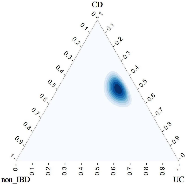
For the control group, nonnIBD, there does not exist evidence to reject the null hypothesis of marginal homogeneity. Therefore we do not detect any systematic errors in this category;

2.

For UC, the test,

$$\left\{\begin{array}{cc}{H}_0:& p_{UC}\le 0.5\\ H_1:& p_{UC}>0.5,\end{array}\right.$$

(26)

with $p_{UC}=P[A\_UC\cap P\_Others]$. It is obtained p-value $=9.7e-07$, and therefore the null hypothesis is rejected, which suggests underprediction of the UC category.

3.

For CD, the test,

$$\left\{\begin{array}{cc}{H}_0:& p_{CD}\ge 0.5\\ H_1:& p_{CD}<0.5,\end{array}\right.$$

(27)

with $p_{CD}=P[A\_CD\cap P\_Others]$, $p-\mathrm{value}=0.0012$ is obtained, which suggests overprediction of CD disease.

Since in this example we have evidence of problems of misclassification, the next step is to assess the conditional probabilities of interest.

5.3.2. Bayesian Approach

In this case, a noninformative prior distribution is first considered. Since other possibilities are also possible, later a sequential use of Bayes is illustrated.

Noninformative Prior Distributions

Let us consider a prior Dirichlet distribution with ${\alpha }_j=1\forall j=1,\cdots ,3$, as in previous applications the Bayes estimates of conditional probabilities are obtained along with the variances and standards deviations of marginal distributions. As novelty in this application, we highlight that since we are dealing with $r=3$ categories, the posterior distribution associated to each category can be represented in the two-dimensional simplex, which allows a visual analysis of these joint distributions. To obtain the graphical representation in the two-dimensional simplex, 1000 values have been generated by using the R software, a grid has been established and the corresponding contour plots have been displayed.

From results in Table 27, we highlight that

$$\widehat{P}[P\_nonIBD|A\_nonIBD]=0.6786\mathrm{and}\widehat{P}[P\_CD|A\_nonIBD]=0.2857.$$

Table 27. Bayesian summaries in $\mathbf{A}\_\mathbf{nonIBD}$.

	${\mathit{n}}_{1+}$	${\mathit{\alpha }}_1$	${\tilde{\mathit{\alpha }}}_1$	${\widehat{\mathit{\theta }}}_{{\mathit{j}}_{\mathit{b}}}$	$\mathbf{Var}\left({\mathit{\theta }}_{\mathit{j}}\right|{\tilde{\mathit{\alpha }}}_1)$	$\mathbf{sd}\left({\mathit{\theta }}_{\mathit{j}}\right|{\tilde{\mathit{\alpha }}}_1)$
P_nonIBD	37	1	38	0.6785714	0.0038265	0.0618590
P_UC	1	1	2	0.0357143	0.0006042	0.0245803
P_CD	15	1	16	0.2857143	0.0035804	0.0598363

Although in the control group, $non\_IBD$, there is no evidence of classification bias, the estimated probability of being classified as CD is relatively high. As for the plot given in Figure 1, note that the joint posterior distribution is quite concentrated and close to $non\_IBD$ vertex. The mode of this posterior distribution can also be given as Bayes estimates of the conditional probabilities, these are:

$$\widehat{P}[P\_nonIBD|A\_nonIBD]=0.6981,\widehat{P}[P\_UC|A\_nonIBD]=0.0189,$$

and $\widehat{P}[P\_CD|A\_nonIBD]=0.2830.$ These estimates are quite close to the previous ones.

Figure 1. Posterior Dirichlet in A_nonIBD.

In the $A\_UC$ category, Table 28, we found that, $\widehat{P}[P\_UC|A\_UC]=0.3704$ is quite low, and $\widehat{P}[P\_CD|A\_UC]=0.5000$, that is, the estimated probability of an individual with UC to be diagnosed as CD is surprisingly high.

Table 28. Bayesian summaries in $\mathbf{A}\_\mathbf{UC}$.

	${\mathit{n}}_{2+}$	${\mathit{\alpha }}_2$	${\tilde{\mathit{\alpha }}}_2$	${\widehat{\mathit{\theta }}}_{{\mathit{j}}_{\mathit{b}}}$	$\mathbf{Var}\left({\mathit{\theta }}_{\mathit{j}}\right|{\tilde{\mathit{\alpha }}}_2)$	$\mathbf{sd}\left({\mathit{\theta }}_{\mathit{j}}\right|{\tilde{\mathit{\alpha }}}_2)$
P_nonIBD	6	1	7	0.1296296	0.0020514	0.0452921
P_UC	19	1	20	0.3703704	0.0042399	0.0651147
P_CD	26	1	27	0.5000000	0.0045455	0.0674200

As for the joint posterior distribution plotted in Figure 2, we highlight that the area of highest posterior density is closer to the CD vertex than to UC vertex. This is coherent with the result in test (26), and confirms the underprediction of UC category in favour of CD.

Figure 2. Posterior Dirichlet in A_UC.

The mode of this posterior distribution is:

$$\widehat{P}[P\_nonIBD|A\_UC]=0.1176,\widehat{P}[P\_UC|A\_UC]=0.3725,\widehat{P}[P\_CD|A\_UC]=0.5098.$$

Again, these estimates are quite close to the previous ones.

Finally, let us study the CD category in Table 29.

Table 29. Bayesian summaries in $\mathbf{A}\_\mathbf{CD}$.

	${\mathit{n}}_{3+}$	${\mathit{\alpha }}_3$	${\tilde{\mathit{\alpha }}}_3$	${\widehat{\mathit{\theta }}}_{{\mathit{j}}_{\mathit{b}}}$	$\mathbf{Var}\left({\mathit{\theta }}_{\mathit{j}}\right|{\tilde{\mathit{\alpha }}}_3)$	$\mathbf{sd}\left({\mathit{\theta }}_{\mathit{j}}\right|{\tilde{\mathit{\alpha }}}_3)$
P_nonIBD	15	1	16	0.1632653	0.0013799	0.0371470
P_UC	3	1	4	0.0408163	0.0003955	0.0198861
P_CD	77	1	78	0.7959184	0.0016407	0.0405059

We highlight that the estimated probability of the right classification is the highest one, $\widehat{P}[P\_CD|A\_CD]=0.7959,$ and the area of highest posterior density is close to CD vertex, see Figure 3. The mode of Figure 3 is $(0.1579,0.0316,0.8106)$.

Figure 3. Posterior Dirichlet in A_CD.

All these facts allow us to conclude that there exists a serious problem of overprediction of CD and underprediction of UC. To asses this fact estimates of conditional probabilities have been given. As for the joint posterior distributions, note that for $A\_nonIBD$ and $A\_CD$, they are close to the corresponding vertex as it can be seen in Figure 1 and Figure 3 respectively, which is good for a right classification. However, for $A\_UC$ is clear the confusion with the category CD, see Figure 2.

For completeness, $95\%$ credible intervals are given in Appendix A along with results for a uniform discrete prior in r points.

5.3.3. Sequential Use of Bayes Theorem

In this subsection, it is shown that if new information is available then the Bayes theorem can be used in a sequential way to update our beliefs. Moreover our estimates exhibit less variability as it next illustrated.

Step 1, (confusion matrix $M_1$). Consider the Dirichlet-multinomial model for every row in a $r\times r$ confusion matrix, denoted as $M_1$. That is, for $k=1,\dots ,r$, we have a prior Dirichlet distribution for ${\mathit{\theta }}_k$,

$${\mathit{\theta }}_k|{\alpha }_k\sim Dirichlet\left({\alpha }_k\right),$$

and ${\mathbf{Y}}_k=(Y_{1|k},\dots ,Y_{r|k})$, the kth row with the counts in $M_1$, is distributed as

$${\mathbf{Y}}_k|n_{k+}^{step1},{\mathit{\theta }}_k\sim Multinomial(n_{k+}^{step1},{\mathit{\theta }}_k).$$

Given ${\mathbf{y}}_k^{obs}$, the posterior distribution for ${\mathit{\theta }}_k$ is

$${\mathit{\theta }}_{\mathbf{k}}|{\mathbf{y}}_k^{obs},{\alpha }_{\mathbf{k}}\sim Dirichlet\left(n_{1|k}^{step1}+{\alpha }_{1|k},\cdots ,n_{r|k}^{step1}+{\alpha }_{r|k}\right).$$

(28)

Step 2, (confusion matrix $M_2$). If, in the same problem of classification, a new confusion matrix, $M_2$ is obtained in a set of independent observations of those considered to build $M_1$, then the distribution given in (28) can be considered as prior in Step 2 to get a new posterior distribution. Specifically, let

$${\mathit{\theta }}_k|{\tilde{\alpha }}_k\sim Dirichlet\left({\tilde{\alpha }}_k\right),$$

and ${\mathbf{W}}_k=(W_{1|k},\dots ,W_{r|k})$ the kth row with the counts in $M_2$, where

$${\mathbf{W}}_k|n_{k+}^{step2},{\mathit{\theta }}_k\sim Multinomial\left(n_{k+}^{step2},{\mathit{\theta }}_k\right)$$

Given ${\mathbf{w}}_k^{obs}$, the posterior distribution for ${\mathit{\theta }}_k$ is

$${\mathit{\theta }}_{\mathbf{k}}|{\mathbf{w}}_k^{obs},{\tilde{\alpha }}_{\mathbf{k}}\sim Dirichlet\left(n_{1|k}^{step2}+{\tilde{\alpha }}_{1|k},\cdots ,n_{r|k}^{step2}+{\tilde{\alpha }}_{r|k}\right).$$

(29)

To illustrate the sequential method, let us consider $M_1$ as the matrix given in Table 24 and $M_2$ the matrix given in Table 30.

Table 30. $M_2$ matrix (IBD).

	P_nonIBD	P_UC	P_CD
A_nonIBD	42	1	10
A_UC	22	22	7
A_CD	34	10	51

The different estimates are listed in the following tables.

We highlight the increase of precision we got when the new information is incorporated in the process of estimation. Note that the standard deviations of posterior distributions listed in Table 31, Table 32 and Table 33 are less than those listed in Table 27, Table 28 and Table 29. This is the main merit of the sequential use of Bayes’ theorem.

Table 31. Bayesian summaries Step 2 in $\mathbf{A}\_\mathbf{nonIBD}$.

	${\mathit{n}}_{1+}^{\mathbf{step}2}$	${\tilde{\mathit{\alpha }}}_1$	${\tilde{\mathit{\alpha }}}_1^{\mathbf{step}2}$	${\widehat{\mathit{\theta }}}_{{\mathit{j}}_{\mathit{b}}}$	$\mathbf{Var}\left({\mathit{\theta }}_{\mathit{j}}\right|{\tilde{\mathit{\alpha }}}_1^{\mathbf{step}2})$	$\mathbf{sd}\left({\mathit{\theta }}_{\mathit{j}}\right|{\tilde{\mathit{\alpha }}}_1^{\mathbf{step}2})$
P_nonIBD	42	38	80	0.7339450	0.0017752	0.0421329
P_UC	1	2	3	0.0275229	0.0002433	0.0155988
P_CD	10	16	26	0.2385321	0.0016512	0.0406352

Table 32. Bayesian summaries Step 2 in $\mathbf{A}\_\mathbf{UC}$.

	${\mathit{n}}_{2+}^{\mathbf{step}2}$	${\tilde{\mathit{\alpha }}}_2$	${\tilde{\mathit{\alpha }}}_2^{\mathbf{step}2}$	${\widehat{\mathit{\theta }}}_{{\mathit{j}}_{\mathit{b}}}$	$\mathbf{Var}\left({\mathit{\theta }}_{\mathit{j}}\right|{\tilde{\mathit{\alpha }}}_2^{\mathbf{step}2})$	$\mathbf{sd}\left({\mathit{\theta }}_{\mathit{j}}\right|{\tilde{\mathit{\alpha }}}_2^{\mathbf{step}2})$
P_nonIBD	22	7	29	0.2761905	0.0018859	0.0434274
P_UC	22	20	42	0.4000000	0.0022642	0.0475831
P_CD	7	27	34	0.3238095	0.0020656	0.0454492

Table 33. Bayesian summaries Step 2 in $\mathbf{A}\_\mathbf{CD}$.

	${\mathit{n}}_{3+}^{\mathbf{step}2}$	${\tilde{\mathit{\alpha }}}_3$	${\tilde{\mathit{\alpha }}}_3^{\mathbf{step}2}$	${\widehat{\mathit{\theta }}}_{{\mathit{j}}_{\mathit{b}}}$	$\mathbf{Var}\left({\mathit{\theta }}_{\mathit{j}}\right|{\tilde{\mathit{\alpha }}}_3^{\mathbf{step}2})$	$\mathbf{sd}\left({\mathit{\theta }}_{\mathit{j}}\right|{\tilde{\mathit{\alpha }}}_3^{\mathbf{step}2})$
P_nonIBD	34	16	50	0.2590674	0.0009894	0.0314554
P_UC	10	4	14	0.0725389	0.0003468	0.0186223
P_CD	51	78	129	0.6683938	0.0011425	0.0338008

6. Discussion

The aim of this paper is to propose methods to detect the bias of classification, as well as overprediction and underprediction problems associated to categories in a confusion matrix. The methods may be applied to confusion matrices obtained as result of applying supervised learning algorithms, such as logistic regression, linear and quadratic discriminant analysis, naive Bayes, k-nearest neighbors, classification trees, random forests, boosting or support vector machines, among others. First marginal homogeneity tests are introduced. They are based on applying techniques to matched pairs of observations tailored to this context. Second, a Bayesian methodology, based on the multinomial-Dirchlet distribution is developed, which allows us to confirm and to assess the magnitudes of these problems by using prior information. Three applications taken from peer-reviewed and different scientific literature have been carried out. They illustrate relevant aspects related to the performance of our proposal, mainly varying the dimension r of the confusion matrix. In all of them, the results obtained have been satisfactory. We consider that these new methods are of interest for a better definition of classes, to improve the performance of classification methods, and to assess the global process of classification. As for related work, we highlight the results given in [22], where an excellent review of metrics to deal with multi-class classification tasks is given. There, usual indicators such as accuracy, recall, F1-Score, and kappa coefficients, among others along with their properties can be found. In this sense, we highlight that the Bayesian results given in Section 4 can be used as a micro method, with the additional merit of providing measurements about the variability of summaries proposed. In this sense, the standard deviation of posterior distributions can be used. To carry out a comparison of the results in our paper to existing metrics can be of interest in future works. Additionally, we intend to depply study the structure of confusions, for instance, to analyze if certain classes have a common confusion structure or not, their relationships, the effect of the sample size, or dealing with unbalanced classes.

References

- Goin, J.E. Classification Bias of the k-Nearest Neighbor Algorithm. IEEE Trans. Pattern Anal. Mach. Intell. 1984, PAMI-6, 379–381. [Google Scholar] [CrossRef] [PubMed]
- Black, S.; Gonen, M. A Generalization of the Stuart-Maxwell Test. In SAS Conference Proceedings: South-Central SAS Users Group 1997; Applied Logic Associates, Inc.: Houston, TX, USA, 1997. [Google Scholar]
- Sun, X.; Yang, Z. Generalized McNemar’s Test for Homogeneity of the Marginal Distributions. In Proceedings of the SAS Global Forum Proceedings, Statistics and Data Analysis, San Antonio, TX, USA, 16–19 March 2008; Volume 382, pp. 1–10. [Google Scholar]
- Hastie, T.; Tibshirani, R.; Friedman, J.H. The Elements of Statistical Learning: Data Mining, Inference, and Prediction, 2nd ed.; Springer: New York, NY, USA, 2009. [Google Scholar]
- Barranco-Chamorro, I.; Luque-Calvo, P.; Jiménez-Gamero, M.; Alba-Fernández, M. A study of risks of Bayes estimators in the generalized half-logistic distribution for progressively type-II censored samples. Math. Comput. Simul. 2017, 137, 130–147. [Google Scholar] [CrossRef]
- Congalton, R.G.; Green, K. Assessing the Accuracy of Remotely Sensed Data. Principles and Practices, 3rd ed.; CRC Press: Boca Raton, FL, USA, 2020. [Google Scholar]
- Carrillo-García, R.M. Text Mining: Principios Básicos, Aplicaciones, Técnicas y Casos Prácticos. Master’s Thesis, Universidad de Sevilla, Sevilla, Spain, 2021. [Google Scholar]
- Carrillo-García, R.M. Algorithms and Applications in Statistical Data Mining; PI3: Programa IMUS de Iniciación a la Investigación; Instituto de Matemáticas de la Universidad de Sevilla: Sevilla, Spain, 2021. [Google Scholar]
- Huang, Q.; Zhang, X.; Hu, Z. Application of Artificial Intelligence Modeling Technology Based on Multi-Omics in Noninvasive Diagnosis of Inflammatory Bowel Disease. J. Inflamm. Res. 2021, 14, 1933–1943. [Google Scholar] [CrossRef] [PubMed]
- Liu, C.; Frazier, P.; Kumar, L. Comparative Assessment of the Measures of Thematic Classification Accuracy. Remote Sens. Environ. 2007, 107, 606–616. [Google Scholar] [CrossRef]
- Pontius, R.; Millones, M. Death to Kappa: Birth of quantity disagreement and allocation disagreement for accuracy assessment. Int. J. Remote Sens. 2011, 32, 4407–4429. [Google Scholar] [CrossRef]
- Lance, R.F.; Kennedy, M.L.; Leberg, P.L. Classification Bias in Discriminant Function Analyses used to Evaluate Putatively Different Taxa. J. Mammal. 2000, 81, 245–249. [Google Scholar] [CrossRef] [Green Version]
- Schmidt, R.L.; Walker, B.S.; Cohen, M.B. Verification and classification bias interactions in diagnostic test accuracy studies for fine-needle aspiration biopsy. Cancer Cytopathol. 2015, 123, 193–201. [Google Scholar] [CrossRef] [PubMed] [Green Version]
- Rivas-Ruiz, F.; Pérez-Vicente, S.; González-Ramírez, A. Bias in clinical epidemiological study designs. Allergol. Immunopathol. 2013, 41, 54–59. [Google Scholar] [CrossRef] [PubMed]
- Barranco-Chamorro, I.; Muñoz Armayones, S.; Romero-Losada, A.; Romero-Campero, F. Multivariate Projection Techniques to Reduce Dimensionality in Large Datasets. In Smart Data. State-of-the-Art Perspectives in Computing and Applications; CRC Press, Taylor & Francis Group: Boca Raton, FL, USA, 2019. [Google Scholar]
- Tsendbazar, N.; de Bruin, S.; Mora, B.; Schouten, L.; Herold, M. Comparative assessment of thematic accuracy of GLC maps for specific applications using existing reference data. Int. J. Appl. Earth Obs. Geoinf. 2016, 44, 124–135. [Google Scholar] [CrossRef]
- Pérez, C.J.; Girón, F.J.; Martín, J.; Ruiz, M.; Rojano, C. Misclassified multinomial data: A Bayesian approach. Rev. Real Acad. Cienc. Exactas Fís. Nat. Ser. A Mat. (RACSAM) 2007, 101, 71–80. [Google Scholar]
- R Core Team. R: A Language and Environment for Statistical Computing; R Foundation for Statistical Computing: Vienna, Austria, 2021. [Google Scholar]
- Meredith, M.; Kruschke, J. HDInterval: Highest (Posterior) Density Intervals. R Package Version 0.2.2. 2020. Available online: https://cran.r-project.org/web/packages/HDInterval/index.html (accessed on 12 July 2021).
- Signorell, A.; Aho, K.; Alfons, A.; Anderegg, N.; Aragon, T.; Arachchige, C.; Arppe, A.; Baddeley, A.; Barton, K.; Bolker, B.; et al. DescTools: Tools for Descriptive Statistics. R Package Version 0.99.44. 2021. Available online: https://cran.r-project.org/web/packages/DescTools/index.html (accessed on 12 December 2021).
- Tsagris, M.; Athineou, G. Compositional: Compositional Data Analysis. R Package Version 4.8. 2021. Available online: https://cran.r-project.org/web/packages/Compositional/index.html (accessed on 10 August 2021).
- Grandini, M.; Bagli, E.; Visani, G. Metrics for Multi-Class Classification: An Overview. arXiv 2020, arXiv:2008.05756. [Google Scholar]
- McNemar, Q. Note on the sampling error of the difference between correlated proportions or percentages. Psychometrika 1947, 12, 153–157. [Google Scholar] [CrossRef] [PubMed]
- Edwards, A. Note on the “correction for continuity” in testing the significance of the difference between correlated proportions. Psychometrika 1948, 13, 185–187. [Google Scholar] [CrossRef] [PubMed]
- Balakrishnan, N.; Johnson, N.L.; Kotz, S. Multinominal Distributions. In Discrete Multivariate Distributions; Series in Probability and Statistics; Wiley: Hoboken, NJ, USA, 1997; Chapter 2. [Google Scholar]
- Kotz, S.; Balakrishnan, N.; Johnson, N.L. Dirichlet and Inverted Dirichlet Distributions. In Continuous Multivariate Distributions: Models and Applications; Series in Probability and Statistics; Wiley: Hoboken, NJ, USA, 2000; Volume 1, Chapter 49; pp. 458–527. [Google Scholar] [CrossRef]
Publisher’s Note: MDPI stays neutral with regard to jurisdictional claims in published maps and institutional affiliations. |
© 2021 by the authors. Licensee MDPI, Basel, Switzerland. This article is an open access article distributed under the terms and conditions of the Creative Commons Attribution (CC BY) license (https://creativecommons.org/licenses/by/4.0/).