Article

Modeling Uncertainty in Fracture Age Estimation from Pediatric Wrist Radiographs

1
Department of Computer Engineering, Faculty of Engineering, University of Rijeka, Vukovarska 58, Rijeka 51000, Croatia
2
Division of General Radiology, Department of Radiology, Medical University of Graz, 8036 Graz, Austria
3
Center for Artificial Intelligence and Cybersecurity, University of Rijeka, Radmile Matejčić 2, Rijeka 51000, Croatia
4
Division of Pediatric Radiology, Department of Radiology, Medical University of Graz, 8036 Graz, Austria
*
Author to whom correspondence should be addressed.
Mathematics 2021, 9(24), 3227; https://doi.org/10.3390/math9243227
Submission received: 16 November 2021 / Revised: 11 December 2021 / Accepted: 12 December 2021 / Published: 14 December 2021
(This article belongs to the Section Mathematics and Computer Science)

Abstract

:
In clinical practice, fracture age estimation is commonly required, particularly in children with suspected non-accidental injuries. It is usually done by radiologically examining the injured body part and analyzing several indicators of fracture healing such as osteopenia, periosteal reaction, and fracture gap width. However, age-related changes in healing timeframes, inter-individual variabilities in bone density, and significant intra- and inter-operator subjectivity all limit the validity of these radiological clues. To address these issues, for the first time, we suggest an automated neural network-based system for determining the age of a pediatric wrist fracture. In this study, we propose and evaluate a deep learning approach for automatically estimating fracture age. Our dataset included 3570 medical cases with a skewed distribution toward initial consultations. Each medical case includes a lateral and anteroposterior projection of a wrist fracture, as well as patients’ age, and gender. We propose a neural network-based system with Monte-Carlo dropout-based uncertainty estimation to address dataset skewness. Furthermore, this research examines how each component of the system contributes to the final forecast and provides an interpretation of different scenarios in system predictions in terms of their uncertainty. The examination of the proposed systems’ components showed that the feature-fusion of all available data is necessary to obtain good results. Also, proposing uncertainty estimation in the system increased accuracy and F1-score to a final 0.906 ± 0.011 on a given task.

1. Introduction

Knowing the approximate age of a bone fracture is a medically and forensically relevant issue, especially in the context of suspected non-accidental trauma in a child. Physicians often request radiologists to estimate the age of a specific fracture, which still might not clearly be answerable in many situations.
Radiography can help estimating a fracture’s age due to specific changes in a fracture’s appearance or through the presence of reparative processes. These processes include mechanisms like soft-tissue swelling in the early, and osteopenia or periosteal reaction in the later phases of healing. In the end, typically after a few months, a fracture is fully remodeled and ceases to be visible. Systematic evaluation of the the published literature revealed that radiographic characteristics of bone healing differ substantially across individual investigations [1]. Radiologically, digital radiography (DR) and computed tomography (CT) are used for fracture detection, and subsequently for estimating fracture age [2]. In adults, fracture healing proceeds in a relatively uniform manner so that the fracture age can be approximated based on the radiological findings [3]. In children, however, fracture healing is primarily dependent on patient age, but may also show inter-individual variabilities. As a result, determining fracture age in pediatric patients is more difficult and lacks a sufficient quantity of consistent data in the literature [3,4,5]. It also leads to a certain degree of skewness within related datasets.
Researchers successfully used artificial intelligence (AI), and specifically deep learning (DL) algorithms automatically classifying medical images in the last years [6]. Computer vision (CV) competed with, and in some studies, even exceeded human experts in fracture detection on X-ray studies [7,8,9]. AI also achieved striking results, transforming images from one domain to another or enhancing medical images by, e.g., suppressing plaster casts from them [10,11]. The backbone of the cited related manuscripts, and many other AI-related studies in medical diagnostics, are neural networks (NN) [12]. Although NNs are highly successful in performing numerous tasks, the explainability of their predictions remains their biggest drawback [13,14]. Hence, a good medical decision support system must provide as much information about the origin of its decisions as possible.
To the best of our knowledge, no DL algorithm has yet been developed to estimate or even determine pediatric fracture ages. The wrist is the most common region of pediatric fractures, leading to a sufficient availability of data [15]. We hypothesize that fracture age estimation can be satisfactorily performed by up-to-date convolutional neural networks (CNN) in pediatric digital wrist radiographs. Therefore, the contributions of our research are as follows:
  • This is the first-ever attempt to tackle the issue of estimating pediatric fracture age using AI. Hence, we propose a standard, as well as guidelines for other researchers to follow;
  • By utilizing the Monte-Carlo dropout method, which treats NN as a Gaussian sampling process, we are able to estimate the uncertainty of the proposed system decisions, unveiling prediction certainty to increase trustworthiness;
  • We propose a novel system based on a CNN combining different features obtained from the medical reports/cases to estimate fracture age. The system is general-purpose, and we believe that its design can also be utilized in other research fields as well.

Related Work

As stated in the previous section, to the best of our knowledge, there is no related research investigating the topic of fracture age estimation. So, as the related work, and starting point of our research, we looked at researches dealing with any kind of age/time estimation from the medical images. One of the pioneer studies in estimating bone age from the X-ray hand images is proposed in [16]. The core idea presented in the paper revolved around segmenting the short bones from the image that can help, due to the bone growth, in the age estimation. This idea was followed by Ebner et al. on the hand images generated by medical resonance imaging (MRI). However, they utilized more advanced methods based on the random regression forest method [17]. Similarly, for the age estimation based on the X-ray images of the hand, Thodberg et al. developed The BonXpert method for automated determination of skeletal maturity [18]. One of the key events dealing with bone age estimation is “The RSNA Pediatric Bone Age Machine Learning Challenge” [19]. The challenge is to estimate skeletal age in a curated data set of 14,236 pediatric hand X-ray images. This challenge showed that NNs can be really useful in coping with a given task of bone age estimation. To summarize, many studies estimate the bone age from different body parts (such as wrist [20] or ankle joint [21]) and different modalities (such as MRI [22] or X-ray [23]). Some of the approaches use landmarks, while others are trying to find useful patterns in whole images to estimate the age of the bones (typically by utilizing NNs) [24]. Although our task is to estimate the age of the fracture, the proposed system is greatly inspired by the proposed methods for bone estimation due to the similarity in the nature of the task.

2. Materials and Methods

Next, we present the dataset used in our experiments, the modeling task, and the developed software system.

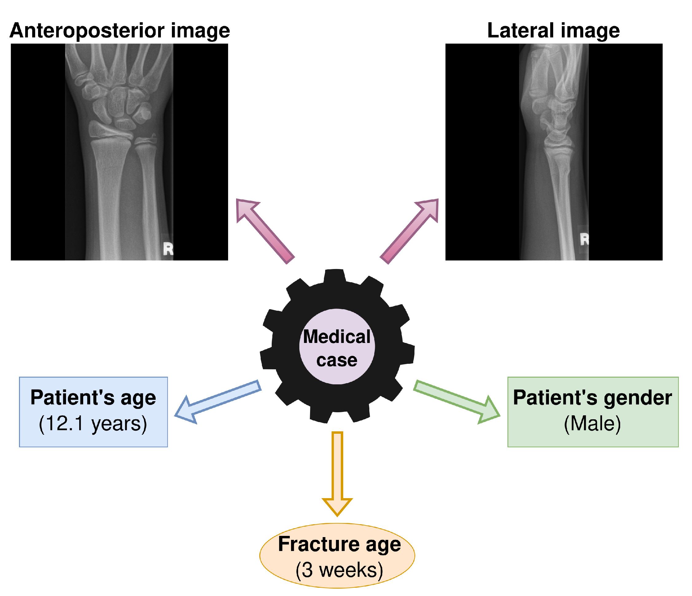
2.1. Dataset and Task Formulation

The dataset originated from the Division of Pediatric Radiology, Department of Radiology, Medical University of Graz, Austria. It contains 3570 digital radiography (DR) studies of pediatric wrists. All data were anonymized, and the images were stored as 16-bit grayscale Portable Network Graphics (PNG) files. The dataset featured comprehensive annotations, including a patient identifier, obfuscated study date and time with preserved relative time intervals, and the information of whether that study was a first presentation to the emergency room or not. DR studies typically contained both anteroposterior (AP) and lateral (LAT) views or projections. In addition to this, one medical case (compare Figure 1) also included patients’ age and gender (male/female) and the age of the fracture in weeks. Hence, the total number of images in the dataset was 7140. There were 2209 male patients with average age of 10.85 ± 3.54 and 1361 female patients with average age of 9.21 ± 3.17 . The wrist fracture age distribution in weeks, calculated between follow-up and initial study, is presented in Figure 2a. As it can be seen, the number of initial exams in which the age of the fracture is 0 weeks old is significantly greater than any other fracture age. This can be explained by the fact that not all injuries need X-ray follow-ups. The number of initial exams was 2418, and the total number of all other exams was 1152. To account for data skewness, we decided to follow the guidelines proposed by Krawczyk and Bartosz [25]. First, we split the data into three meaningful groups based on the fracture age. The first group represents initials exams (0 weeks old fractures), the second group represents around half a month old fractures (1–3 weeks old fractures), while the last group represents fractures older than three weeks. Grouping was done by addressing the same label to all samples belonging to the same group. The described grouping gave the distribution that is shown in Figure 2b. Therefore, the final data distribution used in the research was as follows: group “0 weeks” contained 2418 samples, group “1–3 weeks” 583 samples, and group “3+ weeks” contained 569 samples. From this point on, we tackled the issue of data skewness by adjusting the loss function with the extension of Weighted Cross-Entropy, proposed in [26]. Dataset skewness is substantially influenced by the fact that younger children have lower fracture consolidation times, meaning that older fractures are rarer.
Nevertheless, the dataset skewness is one of the issues that our system tries to overcome. To enhance the credibility of the system, we decided to estimate the uncertainty of its decision making. To summarize, in this paper we provide the system design that estimates the age of the childrens’ wrist fractures based on the X-ray images, patients’ age, and gender. In addition, the system learns and provides uncertainty about the made prediction, which brings us closer towards believable and explainable AI.

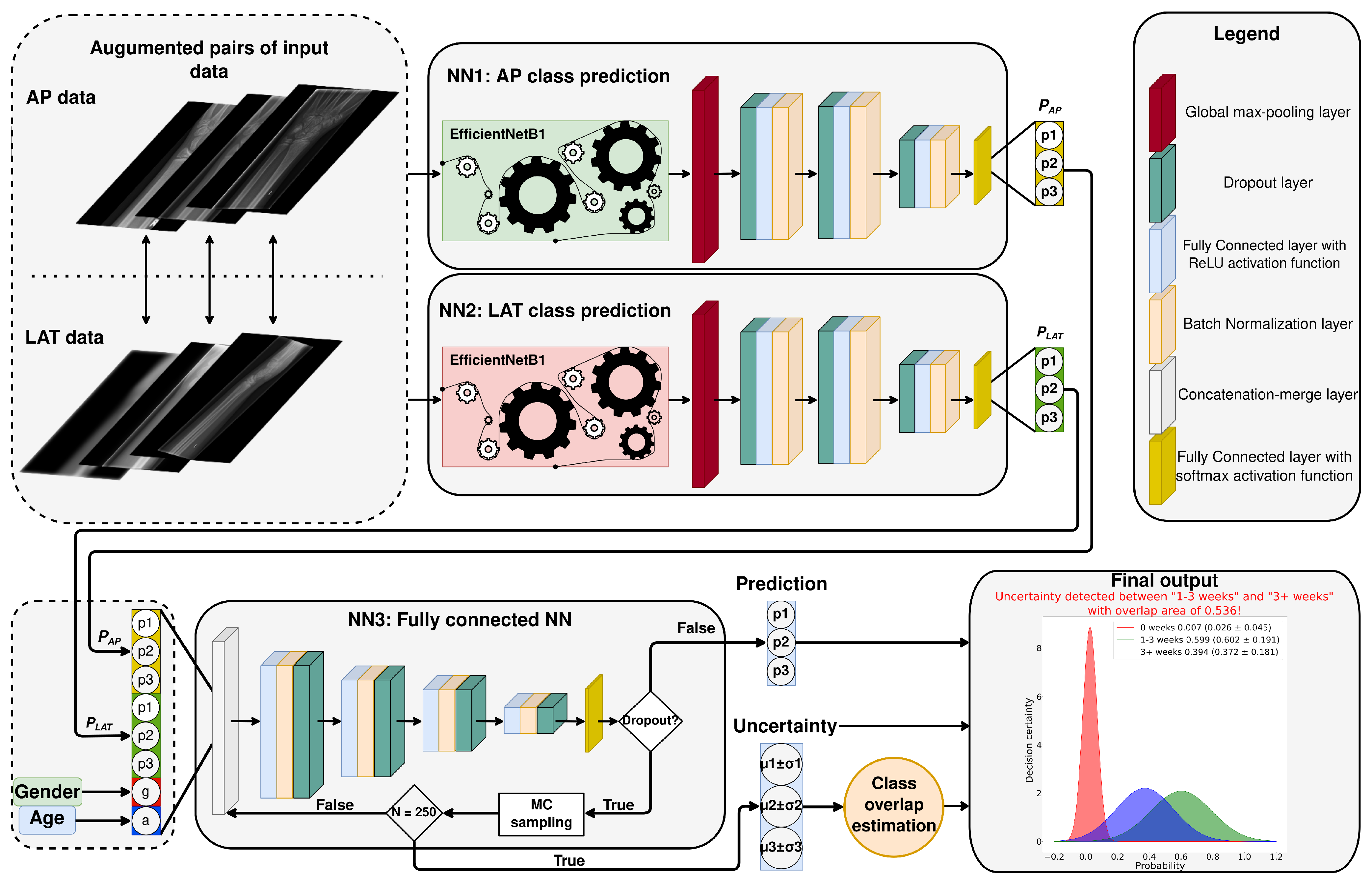
2.2. Proposed System Overview

As mentioned in the related work subsection, the developed system is inspired by “The RSNA Pediatric Bone Age Machine Learning Challenge” [19]. This challenge influenced several papers that were addressing the subject of age estimation from X-ray images [27,28]. Namely, as mentioned previously, to the best of our knowledge there is no related work for fracture age estimation. Hence, we found a similar bone age estimation problem from X-ray images of the hand and took it as a starting point of our proposed system design. All of the solutions presented in challenge have two things in common. The first one is that they use a CNN to extract features from images. The second is supplementing the extracted features with additional information (such as patient age or gender)—encoding all the features in a single vector. Based on the values contained in that vector, the classifier NN head (feed-forward NN) is making predictions. In Figure 3 we present a detailed flowchart of the developed system that has produced the best results in the conducted experiments. As it can be seen, the proposed system has two parts:
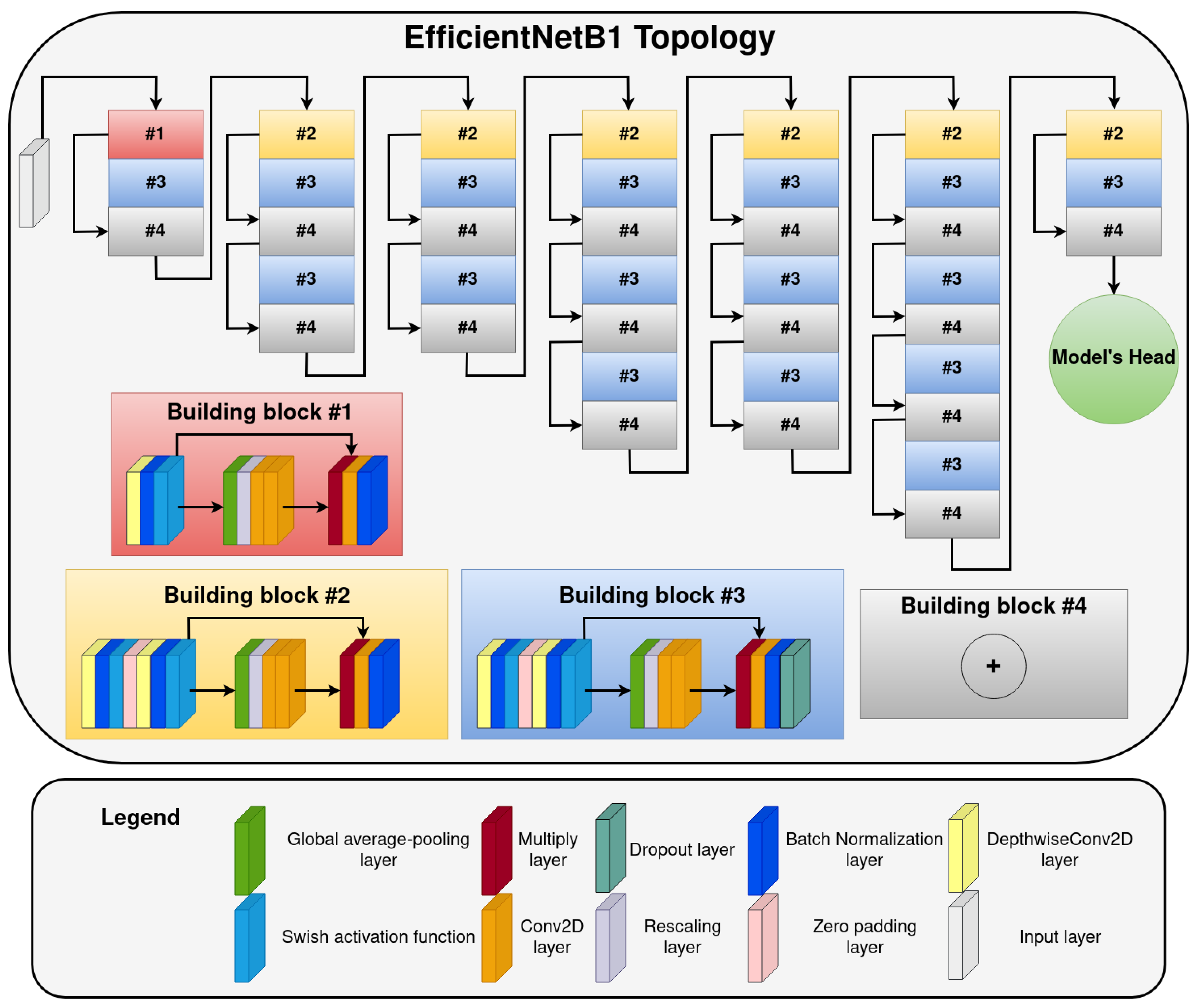
  • The first part of the proposed system has two components—NNs (NN1 and NN2) predicting fracture age based on lateral ( P L A T ) or anteroposterior ( P A P ) input images. The NNs are using EfficientNetB1 (current state-of-the-art NN architecture for classification) as a feature extractor with a custom-developed fully-connected NN head on top of it. The EfficientNetB1 topology (depicted on Figure 4) was the same as that proposed in the original paper (image input size is 240 × 240 pixels) [29], while the fully-connected NN head architecture can be seen in Figure 3. The number of neurons in each dense layer of the NNs head is 1024, 1024, 512, and 3, respectively. The dropout rate in the dropout layers was set to 10 % . The output of each of the two NNs predicts fracture age based on the image it receives as the input. In order to determine if the EfficientNetB1 is the best performing network for our system, we have compared it with other popular deep learning architectures: VGG19 [30], ResNet101 [31], InceptionV3 [32], and Xception [33]. As it can be seen in Appendix B, the EfficientNetB1 was the best performing model of all tested models, and that is why we chose it for our system;
  • The second part of the proposed system is a fully connected NN (NN3) that takes as the input a vector (size 8 × 1 ) created from the outputs of NN1 and NN2, and patient’s gender (g) and age (a). The topology of the NN3 can also be seen in Figure 3. It is constructed from four fully connected layers with 512, 256, 128, and 64 layers, respectively. Dropout rate in the dropout layers was the same as for the first part of the proposed system ( 10 % ). The output of NN3 is a final prediction of the fracture age from the assembly of features. Also, we have employed a decision uncertainty estimation algorithm, which we discuss in the following subsection.

2.2.1. Uncertainty Estimation Algorithm

NNs are generally considered black boxes that lack explainability or any certainty over their decision [34,35]. There are two types of uncertainty: epistemic uncertainty and aleatoric uncertainty. Epistemic uncertainty is the result of limited data and knowledge, while aleatoric uncertainty arises from the stochasticity of observations. Since we cannot influence the input data, we are focused on estimating epistemic uncertainty. The Bayesian approach can be used to some extent to overcome the problem of epistemic uncertainty [36]. Namely, Yarin and Zoubin, in their paper [37] have shown that dropout can be used as a Bayesian approximation of model assembly. In other words, they have proved that a NN with dropout layers is mathematically equivalent to a Bayesian approximation of the Gaussian process [38]. With dropout, each subset of neurons acts as one of k = 250 new NNs that are part of an assembly. Hence, every of the NNs in the assembly has its prediction that can be marked as n n i . The process of generating new NNs can be seen as a Monte Carlo sampling from the original NN. As it can be seen in Equation 1, to obtain the uncertainty prediction for each of the three classes ( c 1 —“0 weeks”, c 2 —“1-3 weeks”, c 3 —“3+ weeks”) we estimate the normal distribution N c defined with the mean μ c and standard deviation σ c of the k = 250 sampled NNs. The μ c and σ c are given in Equations (2) and (3) respectively, and are calculated based on NN1 output P A P , NN2 output P L A T , patient’s gender g, and patient’s age a.
c [ c 1 , c 2 , c 3 ] N c ( μ c , σ c 2 )
μ c = i = 1 k P ( n n i = c P A P , P L A T , g , a ) k
σ c 2 = i = 1 k ( P ( n n i = c P A P , P L A T , g , a ) μ c ) 2 k
That leads to two system outputs: The first one is the prediction of the entire NN, while the second one is the uncertainty output (as depicted in Figure 3). The uncertainty part of the NN is calculated only during prediction. To raise awareness concerning a potential uncertainty, we measured the overlap region between normal distribution curves of two classes having the highest prediction score. If the area of overlap between the two top predicted classes exceeds 50 % , the user receives a warning to verify the plausibility of the output. To obtain the overlapping area between two distributions, we used the algorithm proposed by Linacre [39]. Sampling number k = 250 , representing the number of NNs used in uncertainty estimation, was chosen empirically, based on several trials using different values. We discovered that using more than 250 samples would yield a similar result. On the other hand, the overlapping threshold value of 50 % was taken from related work as a standard (similarly to the IoU threshold value of 0.5 commonly used in object detection tasks).

2.2.2. The Proposed System Training

Due to the relatively small number of data instances (3570), the proposed system is trained by utilizing 5-fold cross-validation [40]. We have also tested 10-fold cross-validation, but it resulted in nearly the same results as the 5-fold cross-validation, only it was more time-consuming (which is why we used 5-folds in the end). Therefore, each of the five disjoint subsets of the available dataset contains 2856 cases for system training, leaving 714 cases for system testing. The proposed system comprises three NNs where the first two NNs’ outputs are part of the input vector for the third NN. Hence, we first trained the first two NNs on lateral and anteroposterior data. We took the necessary precautions to prevent data leakage. Namely, every fold contained data from the same patients’ cases during the sampling process of training and testing data. For instance, if one patient case was in a training set for one of the five folds, it means that both NN1 and NN2 models, as well as NN3, were trained on that particular case. This way, the conclusions based on the NNs results can be compared and discussed because the train and test data (of every fold) had the same source—the same patient/case. Furthermore, we performed the following data augmentation methods over the training data to enhance the versatility of the data and make the trained NNs more robust. For the NNs trained on the images, we used: random flip, random rotation (value in range [ 18 , 18 ] ), brightness and contrast random adjustments, and random cropping of the input image. For the third-fully connected NN (NN3), we did not use any augmentation. The only operation done on the data for the training of the NN3 was scaling the age of the patients to [ 0 , 1 ] range. Data augmentation was not performed on the test sets.
All NNs had the same training hyperparameters (learning rate, batch size, and early-stopping). We investigated a much larger training hyperparameters space using grid search, but the conducted experiments resulted in the same training hyperparameters for all three NNs. Therefore, we used Adam optimizer with learning rate α = 10 4 (chosen from the interval of [ 10 1 , 10 2 , , 10 6 ] ) with batch size 32 (we have also tested the batch size 16, but it had worse performance). We trained NNs for 150 epochs with early stopping after 25 consecutive epochs with no improvements on the test loss function. The loss function was weighted cross-entropy tailored for this purpose and motivated by the work presented in [41]. Reminding ourselves about the obvious data skewness, we increased the weights of rarer classes. We calculated the weight w i of each class using Equation (4). The weight w i is calculated as the ratio of maximum samples of the classes N c i over the number of samples of the class being observed. This procedure resulted in the function W ( x ) shown in Equation (5). The final weighted cross-entropy loss used for system training is given by Equation (6) where y i ^ represents the NN3 output class, y i is the correct class and W ( x ) is a function described in 5 that weighted the loss.
w i = m a x ( N c 1 , N c 2 , N c 3 ) N c i
W ( x ) = 1 f o r x = c 1 4.1475 f o r x = c 2 4.24956 f o r x = c 3
L = i = 0 3 y i · l o g y i ^ · W ( x = y i )
Another approach to address the data skewness is to generate synthetic data for the skewed classes. There are many approaches to do so: from SMOTE algorithm [42] to generative adversarial methods [43]. However, we find these inadequate for the considered problem of fracture age detection from medical images. Namely, since estimating the fracture age is a challenging task even for radiologists, estimating the age of artificial, synthetically added fractures is even more complex and hard to verify. Furthermore, we need to generate a pair of images (LAT and AP) projection, making data synthesis resulting in possible unrealistic cases. Therefore, for this problem, we have chosen a method that does not impair data.

3. Results and Discussion

In this section we present and discuss evaluation results of the proposed system and its components. In Appendix A we provide McNemar’s test results between the proposed system results and its components in the form of five tables—one for each of the five folds [44]. Furthermore, particular attention is set on the uncertainty estimation of the proposed system as well as the interpretation of its results in different situations.

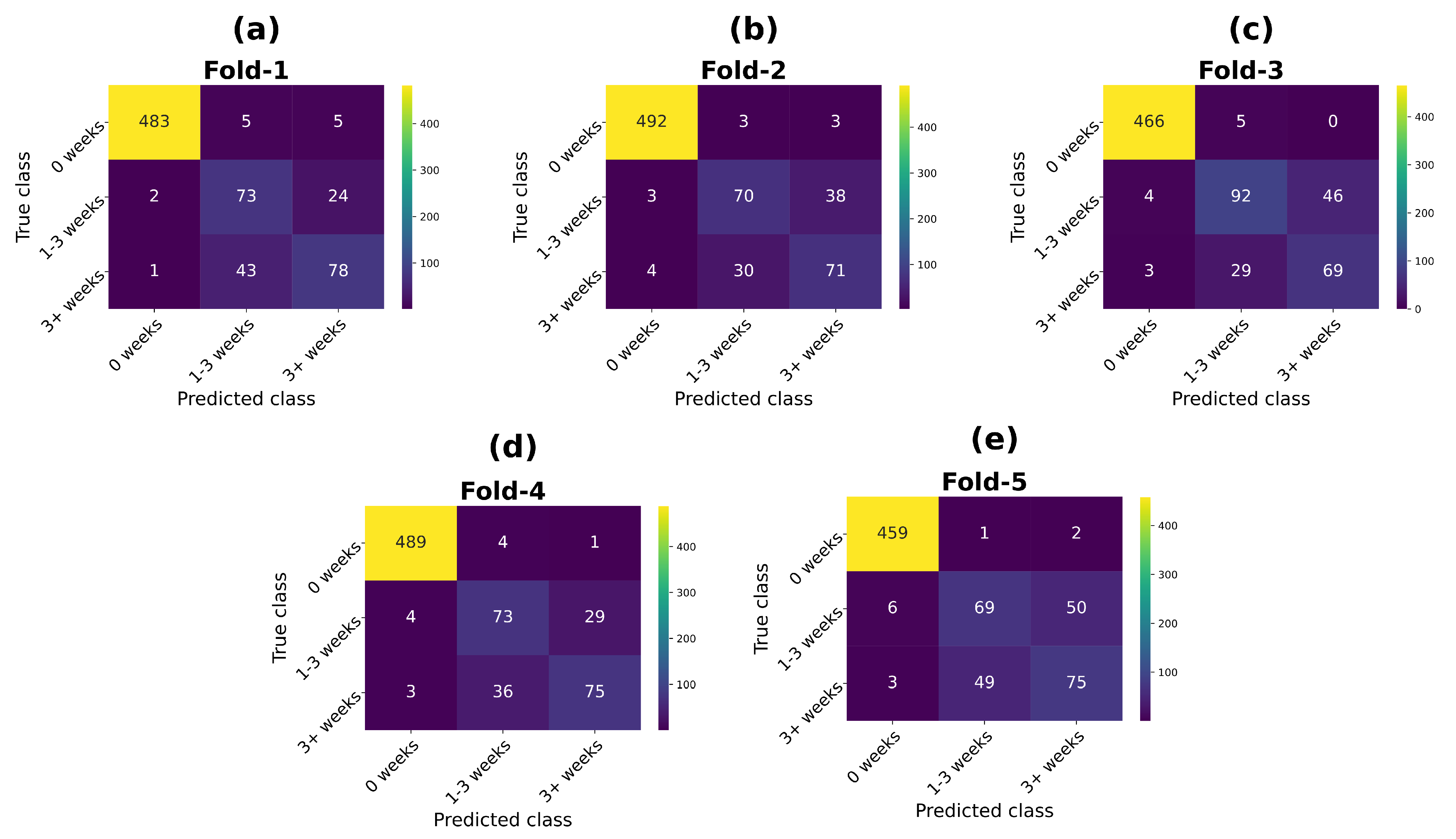
3.1. Proposed System Evaluation Results

To evaluate the proposed system and its components (NNs), we used standard classifier evaluation metrics: precision, recall, F1-Score, and accuracy. Table 1, Table 2 and Table 3 provide results for the proposed system and its components (NN1 and NN2). Results are presented for each of the five folds. Also, we calculated the mean and standard deviation for each metric, which can be considered as an overall score of the NN or system being evaluated. Therefore, in Table 1 we show the results of the NN1 (AP) component of the system. In Table 2 the results of NN2 (LAT) are shown, while Table 3 contains the proposed system’s performance results. By evaluating every component of the system separately, we obtained additional information about their importance and impact on the whole system. According to our expectations, the proposed system performed best on every fold with an overall F1-score of 0.878 ± 0.018 and accuracy of 0.878 ± 0.017 . We can also state that the NN1 (AP) component is more accurate/informative than the NN2 (LAT) component ( 0.858 ± 0.023 F1-score against 0.835 ± 0.012 , respectively). Furthermore, the proposed system obtained ∼2% better results than its best component. The obtained results indicate that the fusion of all possible information is necessary to improve the overall system performance. We have conducted McNemar’s test of the significance between the proposed system and its components to support these claims. The results of McNemar’s test (displayed in tables of Appendix A) show that there is a statistical difference between the proposed system (NN3) and its component on the statistical level p < 0.05 for folds one and three. On the remaining three folds, there is no significant difference between NN3 and NN1, but there is a significant difference between NN3 and NN2. Therefore, although NN3 obtained the best results on all folds (and overall), NN1 could be sufficient to obtain reasonably good results on some folds. However, it will not generalize as well as the proposed system. To depict the severity of the task being solved, we provide the confusion matrices of the proposed system for the five-folds in Figure 5. It can be easily noticed that the proposed system mostly confuses the older fracture which indicates the need for the next step: the evaluation of proposed system uncertainty. Seeing that we are the first ones to tackle the issue of fracture age estimation, there was no other research to compare our results with.

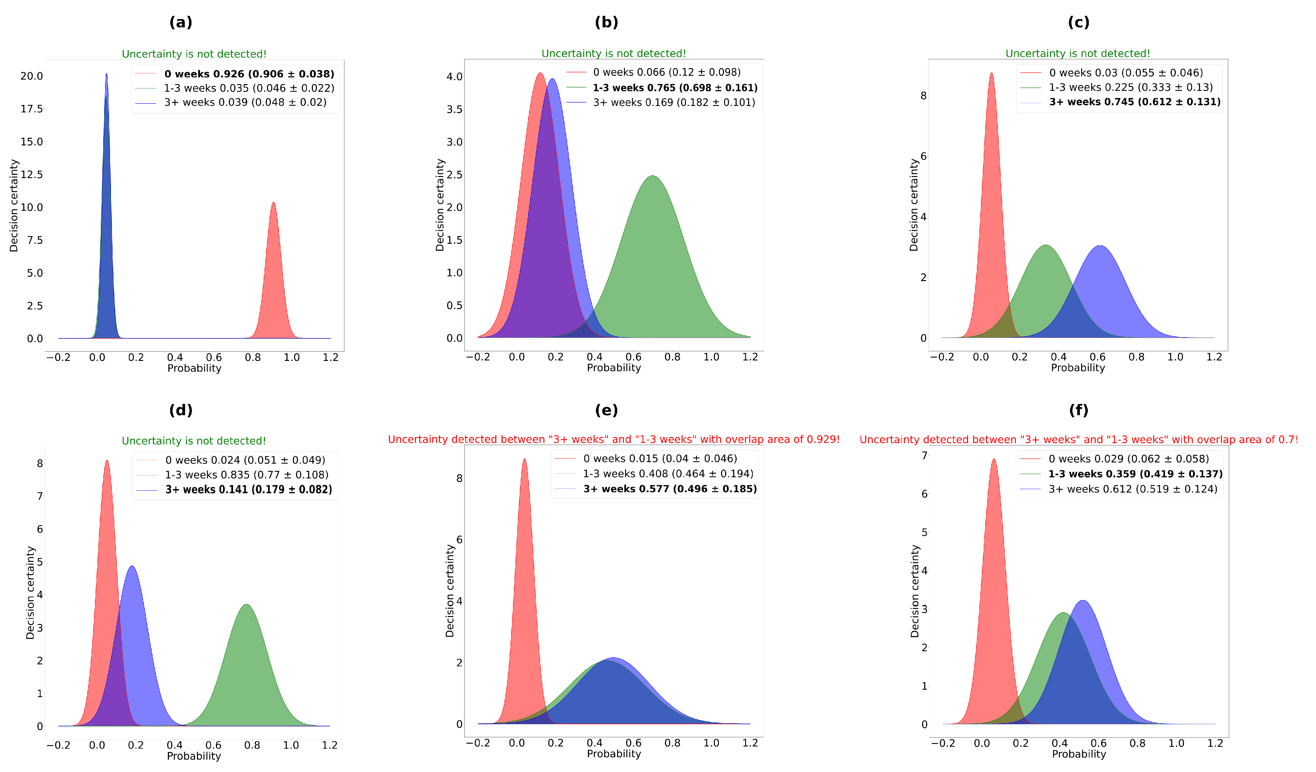
3.2. Uncertainty Estimation Results

We measured the mean and standard deviation of all σ 2 values in every fold to estimate the proposed system’s uncertainty. The measurements were done for each NN component, and for the system as a whole. Also, we divided the measures into two separate groups. The first group is the one where the system or NN component correctly predicted the class, while the second group is the one having erroneous predictions. The expectation is that the subject being evaluated/observed will have smaller uncertainty on the correctly predicted cases and higher uncertainty on the wrongly predicted cases. By comparing the results in Table 4 (correct predictions uncertainty) and Table 5 (wrong predictions uncertainty) we come up with following observations:
  • Both NNs and the proposed system have higher uncertainty on the erroneous predictions than on the correct ones. This is the desired behavior because we want the system to be confident (have the lowest uncertainty) when it is correct and be very uncertain when it makes an erroneous prediction. Also, it is necessary to observe that the biggest difference between overall uncertainty (mean ± stdev) is for the proposed system ( 0.140 0.063 = 0.077 ), which indicates that the system, from this point of view, behaves better than its components;
  • For the correct prediction, the best result was obtained by the NN1 (AP input) with an average uncertainty of 0.034 ± 0.014 . The worse result was obtained by the proposed system ( 0.063 ± 0.015 ). In other words, the proposed system was more uncertain in its correct decision than any of its components, although it obtained the highest F1-score and accuracy (Table 3). This phenomenon, we believe, is due to more inputs/information that the proposed system takes into account;
  • For the erroneous predictions, the proposed system obtained the best results (highest average uncertainty ( 0.140 ± 0.003 ). Analogous to the case of correct predictions, we want the system to be as unsure as possible when making erroneous predictions.
Next, we discuss the interpretability of the proposed system’s predictions. In Figure 6, we depict six scenarios from the perspective of model uncertainty. On the x-axis, we set the probability of the class, while the y-axis shows the decision certainty. In the scenario depicted in Figure 6a, the proposed system has “no doubts” in its decisions. The proposed system predicted class “0 weeks” with 92.6 % probability and a quite high certainty (correct prediction is printed in boldface in the subfigure’s legend). In subfigures (b) and (c), it can be seen that the proposed system gave correct predictions, but the uncertainty of its decision is more considerable than in subfigure (a). Namely, as the overlap between normal distributions representing uncertainty in two classes with the highest probability increases, we can assume that the model could make an erroneous prediction. We set the threshold for system reporting high uncertainty probability to 0.5 , which means that the top two distributions overlap in over 50 % of their areas. By adjusting the mentioned threshold, we are setting up the proposed system sensitivity. For instance, in Figure 6e, the proposed system made a correct prediction but reported high uncertainty about it because of its overlap with another class in 92.9 % . On the other hand, in subfigure (f), the proposed system made an incorrect prediction, but due to the reported uncertainty (overlap of 70 % ), we cannot take its decision for granted. In both cases, we can conclude that we cannot be confident about the models’ prediction, but we can eliminate that the fracture is not a fresh one (0 weeks old) due to the model’s high certainty in that 0 weeks class prediction. Therefore, the system still helped by eliminating the one class. Finally, we need to be aware that the proposed system is not perfect; it can still make mistakes and drive completely wrong predictions with high certainty. This case is depicted in Figure 6d.
We also wanted to inspect the results of the proposed system with regard to its reporting uncertainty. In this case, we considered it a correct prediction if the system reported its uncertainty, and one of the top two classes is the correct one. As it can be seen in Table 6, this adjustment resulted in an increase of the proposed system accuracy and F1-score by ∼2%. The accuracy and F1-score of the proposed system are now both 0.906 ± 0.011 , which, due to the skewness of the data and complexity of the tackled problem, is a decent result. Also, improvement of the proposed system was confirmed by McNemar’s test presented in Appendix A. The results of McNemar’s test show that the proposed system was significantly better (statistical level p < 0.01 ) on all five-folds against its components (NN1 and NN2), as well as NN3 (the proposed system without taking into account reported uncertainty).

3.3. Results Summary

We can summarize the results of our experiments and our observations based on the obtained results in the following:
  • The fusion of the input data in the system results in increased model accuracy, compared independently to any of its components;
  • The amount of uncertainty of the proposed system is greater than the amount of uncertainty of its individual components;
  • The uncertainty in the incorrect predictions of the proposed system is higher than the uncertainty in its correct prediction, which is the desirable system behavior;
  • Uncertainty estimation can help with the output interpretability and can enhance the system usability, especially in cases where the data is poor and very skewed (as was the case with fracture age estimation). Including the uncertainty in the proposed system’s decision increased its average accuracy to ∼90.6%, which can serve as a benchmark point for similar research.
Therefore, the proposed standard yielded by this research employs that we need to use all available data about the patient to develop a good system for fracture age estimation. We have age, gender, and projections available in our case, but the anamnesis could be of great help. The system must focus on each input separately; that is why we have used three neural networks—one neural network that accepts all the data simply would not converge in our case. Furthermore, utilizing the Monte-Carlo dropout method for uncertainty estimation increased not only the accuracy and F1-score but also improved the explainability and plausibility of the whole system. We strongly advise utilizing uncertainty estimation methods when developing computer-aided diagnosis systems that are supposed to be used in real-life practice since they can only result in the benefit of the whole system and its users.

4. Conclusions and Future Work

For the first time, we tackled the issue of fracture age estimation by designing an AI system based on CNNs. Because of skewness in our pediatric wrist radiography dataset, we employed uncertainty estimation as a tool to enhance the proposed system’s accuracy and reliability. Thus, the proposed system becomes more white-box like—providing its decision certainty—which gives a better foundation for the expert using the system to come up with their final decision.
In the future, we are planning on enhancing the proposed system by extracting the regions representing only the fractures and estimating the age of those regions only (instead of the whole images, which is the case now). This way, the proposed system would be more precise and explainable. Also, we plan to solve fracture estimation as a regression problem. Namely, we classified fracture ages in three classes representing clinically relevant intervals in weeks, but fracture age follows a regression curve. To solve this problem entirely, the system needs to be more resistant toward the detected data skewness. To achieve the mentioned goal, we aim to expand the current dataset, and inspect the effect of convolutional filters of the neural networks utilized by the system on the final result. It could also be necessary to introduce some kind of memory in our system to account for rarer instances.

Author Contributions

Conceptualization, F.H., J.L. and S.T.; methodology, F.H., M.J. and S.T.; software, M.J. and F.H.; formal analysis, I.Š. and E.S.; resources, I.Š. and J.L.; writing—original draft preparation, S.T. and F.H.; writing—review and editing, I.Š., J.L. and M.J.; supervision, I.Š. and E.S.; All authors have read and agreed to the published version of the manuscript.

Funding

This work has been supported in part by the Croatian Science Foundation (grant number IP-2020-02-3770) and by the University of Rijeka, Croatia (grant numbers uniri-tehnic-18-17, and uniri-tehnic-18-15).

Institutional Review Board Statement

Not applicable.

Informed Consent Statement

The ethics committee of the Medical University of Graz (IRB00002556) approved the study protocol (No. EK 31-108 ex 18/19). Because of the retrospective data analysis, the committee waived the requirement for informed patient or legal representative consent. We performed all study-related methods in accordance with the Declaration of Helsinki and the relevant guidelines and regulations.

Data Availability Statement

Not applicable.

Conflicts of Interest

The authors declare that they have no conflict of interest.

Appendix A. McNemar’s Test Evaluation of the Proposed System and Its Components

The following tables will show the results of McNemar’s test for the proposed system and its components. The names in the tables represent: NN1 represents EfficientNetB1 model estimating age from AP images, NN2 represents EfficientNetB1 model estimating age from LAT images, NN3 represents the system estimation. In contrast, NN + UNC stands for the system with uncertainty taken into account. Highlighted values in the tables represents statistical significance at the p < 0.05 level. The following tables respectively show results for each of the five folds.
Table A1. McNemar’s test results for the test set of the Fold-1.
Fold-1NN1NN2NN3NN3 + UNC
NN1/0.0450.0080.000
NN20.045/0.0000.000
NN30.0080.000/0.000
NN3 + UNC0.0000.0000.000/
Table A2. McNemar’s test results for the test set of the Fold-2.
Fold-2NN1NN2NN3NN3 + UNC
NN1/0.0020.3590.000
NN20.002/0.0000.000
NN30.3590.000/0.000
NN3 + UNC0.0000.0000.000/
Table A3. McNemar’s test results for the test set of the Fold-3.
Fold-3NN1NN2NN3NN3 + UNC
NN1/0.8610.0260.000
NN20.861/0.0200.000
NN30.0260.020/0.000
NN3 + UNC0.0000.0000.000/
Table A4. McNemar’s test results for the test set of the Fold-4.
Fold-4NN1NN2NN3NN3 + UNC
NN1/0.0400.1550.000
NN20.040/0.0000.000
NN30.1550.000/0.000
NN3 + UNC0.0000.0000.000/
Table A5. McNemar’s test results for the test set of the Fold-5.
Fold-5NN1NN2NN3NN3 + UNC
NN1/0.7020.1410.000
NN20.702/0.0020.000
NN30.1410.002/0.000
NN3 + UNC0.0000.0000.000/

Appendix B. Models Comparison on AP and LAT Data Images

In order to find the best model for fracture age prediction from the anteroposterior (AP) and lateral images (LAT), we have tested several popular deep learning architectures. All architectures were trained and tested with five-fold cross-validation. Furthermore, all tested architectures were trained with Adam optimizer with a batch size of 16 or 32. The learning rate for the Adam optimizer was chosen by performing grid search over the parameter space α [ 10 1 , 10 2 , , 10 6 ] for each tested model. The best hyperparameters combination for every tested model is presented in Table A6. Also, the best combination of hyperparameters for one tested model was the same for LAT and AP data. It is necessary to mention that we have utilized transfer learning for all tested models from ImageNet pre-trained models [45] and the head of the tested models was always the same (the one depicted it Figure 3). To prevent overfitting of the models, we have used early stopping after 25 epochs with no improvements on the test loss function or if the number of epochs trained exceeded 150. In Table A7 and Table A8 we present the average and standard deviation of the model’s performance on the five test folds. The EfficientNetB1 achieved the best scores on LAT data in all metrics with an F1-score of 0.835 ± 0.012 and accuracy of 0.834 ± 0.013 . On the AP data, the EfficientNetB1 model obtained the best F1-score of 0.858 ± 0.023 while the VGG19 model obtained the best accuracy of 0.859 ± 0.014 (the EfficentNetB1 was second best). However, since F1-score is a more general metric (includes false positives and false negatives), we decided to use EfficientNetB1 as the best model and utilize it in our system. Furthermore, due to the difference in parameter number, EfficientNetB1 training duration and memory usage are considerably lower than the VGG19 model, which is another reason to use EfficientNetB1.
Table A6. Models parameters.
ModelLearning RateBatch Size
VGG19 α = 10 5 32
ResNet101 α = 10 4 32
InceptionV3 α = 10 5 32
Xception α = 10 5 32
EfficientNetB1 α = 10 4 32
Table A7. Models comparison on AP data.
ModelPrecisionRecallF1-scoreAccuracy
VGG190.860 ± 0.0150.859 ± 0.0140.856 ± 0.0170.859 ± 0.014
ResNet1010.859 ± 0.0140.845 ± 0.0200.845 ± 0.0180.845 ± 0.020
InceptionV30.849 ± 0.0170.851 ± 0.0140.849 ± 0.0160.851 ± 0.014
Xception0.830 ± 0.0110.824 ± 0.0130.829 ± 0.0100.824 ± 0.013
EfficientNetB10.864 ± 0.0230.857 ± 0.0200.858 ± 0.0230.857 ± 0.020
Table A8. Models comparison on LAT data.
ModelPrecisionRecallF1-scoreAccuracy
VGG190.833 ± 0.0320.823 ± 0.0450.825 ± 0.0390.823 ± 0.045
ResNet1010.835 ± 0.0190.824 ± 0.0230.821 ± 0.0250.824 ± 0.023
InceptionV30.823 ± 0.0130.814 ± 0.0180.816 ± 0.0140.814 ± 0.018
Xception0.812 ± 0.0180.794 ± 0.0330.798 ± 0.0320.794 ± 0.033
EfficientNetB10.841 ± 0.0160.834 ± 0.0130.835 ± 0.0120.834 ± 0.013

References

  1. Messer, D.L.; Adler, B.H.; Brink, F.W.; Xiang, H.; Agnew, A.M. Radiographic timelines for pediatric healing fractures: A systematic review. Pediatr. Radiol. 2020, 50, 1041–1048. [Google Scholar] [CrossRef]
  2. Cappella, A.; de Boer, H.H.; Cammilli, P.; De Angelis, D.; Messina, C.; Sconfienza, L.M.; Sardanelli, F.; Sforza, C.; Cattaneo, C. Histologic and radiological analysis on bone fractures: Estimation of posttraumatic survival time in skeletal trauma. Forensic Sci. Int. 2019, 302, 109909. [Google Scholar] [CrossRef]
  3. Prosser, I.; Maguire, S.; Harrison, S.K.; Mann, M.; Sibert, J.R.; Kemp, A.M. How old is this fracture? Radiologic dating of fractures in children: A systematic review. Am. J. Roentgenol. 2005, 184, 1282–1286. [Google Scholar] [CrossRef] [PubMed] [Green Version]
  4. Halliday, K.E.; Broderick, N.; Somers, J.; Hawkes, R. Dating fractures in infants. Clin. Radiol. 2011, 66, 1049–1054. [Google Scholar] [CrossRef]
  5. Prosser, I.; Lawson, Z.; Evans, A.; Harrison, S.; Morris, S.; Maguire, S.; Kemp, A.M. A timetable for the radiologic features of fracture healing in young children. Am. J. Roentgenol. 2012, 198, 1014–1020. [Google Scholar] [CrossRef] [PubMed]
  6. Erickson, B.J.; Korfiatis, P.; Akkus, Z.; Kline, T.L. Machine learning for medical imaging. Radiographics 2017, 37, 505–515. [Google Scholar] [CrossRef] [PubMed]
  7. Choi, J.W.; Cho, Y.J.; Lee, S.; Lee, J.; Lee, S.; Choi, Y.H.; Cheon, J.E.; Ha, J.Y. Using a dual-input convolutional neural network for automated detection of pediatric supracondylar fracture on conventional radiography. Investig. Radiol. 2020, 55, 101–110. [Google Scholar] [CrossRef]
  8. Gan, K.; Xu, D.; Lin, Y.; Shen, Y.; Zhang, T.; Hu, K.; Zhou, K.; Bi, M.; Pan, L.; Wu, W.; et al. Artificial intelligence detection of distal radius fractures: A comparison between the convolutional neural network and professional assessments. Acta Orthop. 2019, 90, 394–400. [Google Scholar] [CrossRef] [PubMed] [Green Version]
  9. Olczak, J.; Fahlberg, N.; Maki, A.; Razavian, A.S.; Jilert, A.; Stark, A.; Sköldenberg, O.; Gordon, M. Artificial intelligence for analyzing orthopedic trauma radiographs: Deep learning algorithms—Are they on par with humans for diagnosing fractures? Acta Orthop. 2017, 88, 581–586. [Google Scholar] [CrossRef] [Green Version]
  10. Ying, X.; Guo, H.; Ma, K.; Wu, J.; Weng, Z.; Zheng, Y. X2CT-GAN: Reconstructing CT from biplanar X-rays with generative adversarial networks. In Proceedings of the IEEE/CVF Conference on Computer Vision and Pattern Recognition, Long Beach, CA, USA, 15–20 June 2019; pp. 10619–10628. [Google Scholar]
  11. Hržić, F.; Žužić, I.; Tschauner, S.; Štajduhar, I. Cast suppression in radiographs by generative adversarial networks. J. Am. Med Informatics Assoc. 2021, 28, 2687–2694. [Google Scholar] [CrossRef]
  12. Haglin, J.M.; Jimenez, G.; Eltorai, A.E. Artificial neural networks in medicine. Health Technol. 2019, 9, 150–154. [Google Scholar] [CrossRef]
  13. Sorantin, E.; Grasser, M.G.; Hemmelmayr, A.; Tschauner, S.; Hrzic, F.; Weiss, V.; Lacekova, J.; Holzinger, A. The augmented radiologist: Artificial intelligence in the practice of radiology. Pediatr. Radiol. 2021, 688. [Google Scholar] [CrossRef]
  14. Holzinger, A.; Biemann, C.; Pattichis, C.S.; Kell, D.B. What do we need to build explainable AI systems for the medical domain? arXiv 2017, arXiv:1712.09923. [Google Scholar]
  15. Hedström, E.M.; Svensson, O.; Bergström, U.; Michno, P. Epidemiology of fractures in children and adolescents: Increased incidence over the past decade: A population-based study from northern Sweden. Acta Orthop. 2010, 81, 148–153. [Google Scholar] [CrossRef] [PubMed]
  16. Pietka, E.; Gertych, A.; Pospiech, S.; Cao, F.; Huang, H.; Gilsanz, V. Computer-assisted bone age assessment: Image preprocessing and epiphyseal/metaphyseal ROI extraction. IEEE Trans. Med. Imaging 2001, 20, 715–729. [Google Scholar] [CrossRef] [PubMed]
  17. Ebner, T.; Stern, D.; Donner, R.; Bischof, H.; Urschler, M. Towards automatic bone age estimation from MRI: Localization of 3D anatomical landmarks. In Proceedings of the International Conference on Medical Image Computing and Computer-Assisted Intervention, Boston, MA, USA, 14–18 September 2014; pp. 421–428. [Google Scholar]
  18. Thodberg, H.H.; Kreiborg, S.; Juul, A.; Pedersen, K.D. The BoneXpert method for automated determination of skeletal maturity. IEEE Trans. Med Imaging 2008, 28, 52–66. [Google Scholar] [CrossRef]
  19. Halabi, S.S.; Prevedello, L.M.; Kalpathy-Cramer, J.; Mamonov, A.B.; Bilbily, A.; Cicero, M.; Pan, I.; Pereira, L.A.; Sousa, R.T.; Abdala, N.; et al. The RSNA pediatric bone age machine learning challenge. Radiology 2019, 290, 498–503. [Google Scholar] [CrossRef] [PubMed]
  20. Dvorak, J.; George, J.; Junge, A.; Hodler, J. Age determination by magnetic resonance imaging of the wrist in adolescent male football players. Br. J. Sport. Med. 2007, 41, 45–52. [Google Scholar] [CrossRef] [PubMed] [Green Version]
  21. Lu, T.; Shi, L.; Zhan, M.J.; Fan, F.; Peng, Z.; Zhang, K.; Deng, Z.H. Age estimation based on magnetic resonance imaging of the ankle joint in a modern Chinese Han population. Int. J. Leg. Med. 2020, 134, 1843–1852. [Google Scholar] [CrossRef]
  22. Lu, T.; Qiu, L.R.; Ren, B.; Shi, L.; Fan, F.; Deng, Z.H. Forensic age estimation based on magnetic resonance imaging of the proximal humeral epiphysis in Chinese living individuals. Int. J. Leg. Med. 2021, 135, 2437–2446. [Google Scholar] [CrossRef] [PubMed]
  23. Spampinato, C.; Palazzo, S.; Giordano, D.; Aldinucci, M.; Leonardi, R. Deep learning for automated skeletal bone age assessment in X-ray images. Med. Image Anal. 2017, 36, 41–51. [Google Scholar] [CrossRef] [PubMed]
  24. Mughal, A.M.; Hassan, N.; Ahmed, A. Bone age assessment methods: A critical review. Pak. J. Med Sci. 2014, 30, 211. [Google Scholar] [CrossRef] [PubMed]
  25. Krawczyk, B. Learning from imbalanced data: Open challenges and future directions. Prog. Artif. Intell. 2016, 5, 221–232. [Google Scholar] [CrossRef] [Green Version]
  26. Ronneberger, O.; Fischer, P.; Brox, T. U-net: Convolutional networks for biomedical image segmentation. In Proceedings of the International Conference on Medical Image Computing and Computer-Assisted Intervention, Munich, Germany, 5–9 October 2015; pp. 234–241. [Google Scholar]
  27. Lee, J.H.; Kim, Y.J.; Kim, K.G. Bone age estimation using deep learning and hand X-ray images. Biomed. Eng. Lett. 2020, 10, 323. [Google Scholar] [CrossRef] [PubMed]
  28. Widek, T.; Genet, P.; Ehammer, T.; Schwark, T.; Urschler, M.; Scheurer, E. Bone age estimation with the Greulich-Pyle atlas using 3T MR images of hand and wrist. Forensic Sci. Int. 2021, 319, 110654. [Google Scholar] [CrossRef]
  29. Tan, M.; Le, Q. Efficientnet: Rethinking model scaling for convolutional neural networks. In International Conference on Machine Learning; PMLR: Cambridge, MA, USA, 2019; pp. 6105–6114. [Google Scholar]
  30. Simonyan, K.; Zisserman, A. Very deep convolutional networks for large-scale image recognition. arXiv 2014, arXiv:1409.1556. [Google Scholar]
  31. He, K.; Zhang, X.; Ren, S.; Sun, J. Deep residual learning for image recognition. In Proceedings of the IEEE Conference on Computer Vision and Pattern Recognition, Las Vegas, NV, USA, 27–30 June 2016; pp. 770–778. [Google Scholar]
  32. Szegedy, C.; Vanhoucke, V.; Ioffe, S.; Shlens, J.; Wojna, Z. Rethinking the inception architecture for computer vision. In Proceedings of the IEEE Conference on Computer Vision and Pattern Recognition, Las Vegas, NV, USA, 27–30 June 2016; pp. 2818–2826. [Google Scholar]
  33. Chollet, F. Xception: Deep learning with depthwise separable convolutions. In Proceedings of the IEEE Conference on Computer Vision and Pattern Recognition, Honolulu, HI, USA, 21–26 July 2017; pp. 1251–1258. [Google Scholar]
  34. Gawlikowski, J.; Tassi, C.R.N.; Ali, M.; Lee, J.; Humt, M.; Feng, J.; Kruspe, A.; Triebel, R.; Jung, P.; Roscher, R.; et al. A survey of uncertainty in deep neural networks. arXiv 2021, arXiv:2107.03342. [Google Scholar]
  35. Loquercio, A.; Segu, M.; Scaramuzza, D. A general framework for uncertainty estimation in deep learning. IEEE Robot. Autom. Lett. 2020, 5, 3153–3160. [Google Scholar] [CrossRef] [Green Version]
  36. Jospin, L.V.; Buntine, W.; Boussaid, F.; Laga, H.; Bennamoun, M. Hands-on Bayesian Neural Networks–A Tutorial for Deep Learning Users. arXiv 2020, arXiv:2007.06823. [Google Scholar]
  37. Gal, Y.; Ghahramani, Z. Dropout as a bayesian approximation: Representing model uncertainty in deep learning. In International Conference on Machine Learning; PMLR: Cambridge, MA, USA, 2016; pp. 1050–1059. [Google Scholar]
  38. Dudley, R.M. Sample functions of the Gaussian process. Sel. Work. Dudley 2010, 187–224. [Google Scholar] [CrossRef]
  39. Linacre, J.M. Overlapping normal distributions. Rasch Meas. Trans. 1996, 10, 487–488. [Google Scholar]
  40. Fushiki, T. Estimation of prediction error by using K-fold cross-validation. Stat. Comput. 2011, 21, 137–146. [Google Scholar] [CrossRef]
  41. Aurelio, Y.S.; de Almeida, G.M.; de Castro, C.L.; Braga, A.P. Learning from imbalanced data sets with weighted cross-entropy function. Neural Process. Lett. 2019, 50, 1937–1949. [Google Scholar] [CrossRef]
  42. Chawla, N.V.; Bowyer, K.W.; Hall, L.O.; Kegelmeyer, W.P. SMOTE: Synthetic minority over-sampling technique. J. Artif. Intell. Res. 2002, 16, 321–357. [Google Scholar] [CrossRef]
  43. Creswell, A.; White, T.; Dumoulin, V.; Arulkumaran, K.; Sengupta, B.; Bharath, A.A. Generative adversarial networks: An overview. IEEE Signal Process. Mag. 2018, 35, 53–65. [Google Scholar] [CrossRef] [Green Version]
  44. Adedokun, O.A.; Burgess, W.D. Analysis of paired dichotomous data: A gentle introduction to the McNemar test in SPSS. J. Multidiscip. Eval. 2012, 8, 125–131. [Google Scholar]
  45. Huh, M.; Agrawal, P.; Efros, A.A. What makes ImageNet good for transfer learning? arXiv 2016, arXiv:1608.08614. [Google Scholar]
Figure 1. Example of one medical case that consists of Patient’s age and gender, anteroposterior and lateral image, and fracture age.
Mathematics 09 03227 g001
Figure 2. Histograms representing the distribution of data used in the research. In subfigure (a), we present the distribution of a fracture’s age over the weeks. In subfigure (b), we depict a histogram of the same data after grouping the data into three groups.
Mathematics 09 03227 g002
Figure 3. Flowchart of the proposed system.
Mathematics 09 03227 g003
Figure 4. EfficientNetB1 topology. The topology is complex and more details about it can be found in the original paper [29].
Mathematics 09 03227 g004
Figure 5. Confusion matrices depict the proposed system performance. The subfigures (ae) shows confusion matrices for fold one, two, three, four, and five, respectively.
Mathematics 09 03227 g005
Figure 6. Possible outputs of the proposed system concerning uncertainty. Subfigure (a) depicts a scenario with no uncertainty detected. Subfigures (b,c) depict two scenarios with an uncertainty overlap between the top two predictions, but this uncertainty is smaller than the set threshold of 0.5 . Subfigure (d) depicts a scenario with no uncertainty but with an incorrect prediction. Subfigures (e,f) depict two scenarios with uncertainty detected between the top two predictions. However, in subfigure (e) the system would predict the correct class, while in subfigure (f) it would predict the incorrect one.
Mathematics 09 03227 g006
Table 1. Evaluation results of the NNs trained on AP data.
FoldPrecisionRecallF1-scoreAccuracy
Fold-10.8690.8590.8610.859
Fold-20.8800.8800.8790.880
Fold-30.8660.8490.8550.849
Fold-40.8820.8750.8780.875
Fold-50.8200.8250.8150.825
Mean ± stdev0.864 ± 0.0230.857 ± 0.0200.858 ± 0.0230.857 ± 0.020
Table 2. Evaluation results of the NNs trained on LAT data.
FoldPrecisionRecallF1-scoreAccuracy
Fold-10.8460.8250.8330.825
Fold-20.8440.8330.8360.833
Fold-30.8520.8530.8510.853
Fold-40.8540.8430.8400.843
Fold-50.8110.8180.8130.818
Mean ± stdev0.841 ± 0.0160.834 ± 0.0130.835 ± 0.0120.834 ± 0.013
Table 3. Overall evaluation results of the proposed system’s performance.
FoldPrecisionRecallF1-scoreAccuracy
Fold-10.8940.8880.8900.888
Fold-20.8870.8870.8860.887
Fold-30.8800.8780.8780.878
Fold-40.8920.8920.8920.892
Fold-50.8410.8450.8430.845
Mean ± stdev0.879± 0.0190.878± 0.0170.878± 0.0180.878 ± 0.017
Table 4. Uncertainty estimations of the NNs for theirs correct predictions.
FoldAP resultLateral resultsSystem results
(Mean ± Stdev)(Mean ± Stdev)(Mean ± Stdev)
Fold-10.041 ± 0.0410.051 ± 0.0520.055 ± 0.057
Fold-20.020 ± 0.0350.043 ± 0.0470.066 ± 0.044
Fold-30.053 ± 0.0360.035 ± 0.0410.066 ± 0.053
Fold-40.036 ± 0.0360.046 ± 0.0670.046 ± 0.059
Fold-50.021 ± 0.0300.037 ± 0.0500.086 ± 0.035
Mean ± stdev0.034 ± 0.0140.043 ± 0.0070.063 ± 0.015
Table 5. Uncertainty estimations of the NNs for their erroneous predictions.
FoldAP resultLateral resultsSystem results
(Mean ± Stdev)(Mean ± Stdev)(Mean ± Stdev)
Fold-10.072 ± 0.0220.108 ± 0.0470.138 ± 0.039
Fold-20.081 ± 0.0440.102 ± 0.0280.136 ± 0.031
Fold-30.080 ± 0.0260.085 ± 0.0380.138 ± 0.035
Fold-40.073 ± 0.0210.132 ± 0.0520.141 ± 0.042
Fold-50.073 ± 0.0230.111 ± 0.0380.145 ± 0.029
Mean ± stdev0.076 ± 0.0040.108 ± 0.0170.140 ± 0.003
Table 6. Evaluation results of the proposed system with uncertainty taken into account.
FoldPrecisionRecallF1-ScoreAccuracy
Fold-10.9130.9070.9090.907
Fold-20.9070.9080.9070.908
Fold-30.9090.9080.9080.908
Fold-40.9190.9190.9180.919
Fold-50.8860.8880.8870.888
Mean ± stdev0.907 ± 0.0120.906 ± 0.0110.906 ± 0.0120.906 ± 0.011
Publisher’s Note: MDPI stays neutral with regard to jurisdictional claims in published maps and institutional affiliations.

