Dynamical Behavior of a New Chaotic System with One Stable Equilibrium

Abstract

This paper reports a simple three-dimensional autonomous system with a single stable node equilibrium. The system has a constant controller which adjusts the dynamic of the system. It is revealed that the system exhibits both chaotic and non-chaotic dynamics. Moreover, chaotic or periodic attractors coexist with a single stable equilibrium for some control parameter based on initial conditions. The system dynamics are studied by analyzing bifurcation diagrams, Lyapunov exponents, and basins of attractions. Beyond a fixed-point analysis, a new analysis known as connecting curves is provided. These curves are one-dimensional sets of the points that are more informative than fixed points. These curves are the skeleton of the system, which shows the direction of flow evolution.

1. Introduction

Finding chaotic systems with novel dynamics is still exciting [1,2]. For the first time, a chaotic system with only one stable equilibrium was presented by Wang and Chen [3]. They added a constant control parameter to the Sprott E chaotic system [4] so that the stability of its equilibrium changed while its chaotic dynamics were preserved. This discovery opened up a new direction in the field of chaos. Recently studying chaotic flows with special structural features and topological features of attractors has been a hot topic [5,6]. For instance, in the category of special structural features, chaotic systems with one stable equilibrium [7,8], with two stable equilibria [9,10], with an infinite number of equilibria [11,12], and with no equilibria, have been studied [13,14]. Chaotic systems with multi-scroll attractors is an example of flows with special topological features [15]. Multistability is an exciting behavior of chaotic flows [16]. Chaotic flows have a vital application in random number generators and image encryption [17,18,19].

Recently amongst chaotic attractors, there has been an intensive study of hidden attractors [20,21]. The emergence of hidden attractors does not correspond with systems equilibria as their basin of attraction does not contain any equilibria [22,23]. Indeed, despite the conventional studies on chaotic systems based on their equilibria, hidden attractors require a new way of explanation [24,25]. To find the hidden attractors and explain how they are constructed, the perpetual points were employed [2,26]. These points are critical points with zero acceleration and non-zero velocity, introduced as candidates to localize hidden attractors. Despite the importance of perpetual points, it was revealed that the idea of localizing hidden attractors by perpetual points could not be a general solution [27]. It is possible that a higher-dimensional method, which is based on zero-dimensional sets of points, helps localize hidden attractors [28]. Gilmore et al. introduced one-dimensional sets of points known as connecting curves that connect fixed points [29]. These connecting curves provide more global information than fixed points. Inspired by their work, the connecting curves of the presented chaotic system are calculated.

In this paper, a new autonomous chaotic oscillator with only one stable equilibrium is introduced. The system has a constant control parameter. The system dynamics and the effect of changing the control parameter are studied by bifurcation analysis, Lyapunov exponent analysis, representing the different basins of attraction, and the calculating connecting curves of the system.

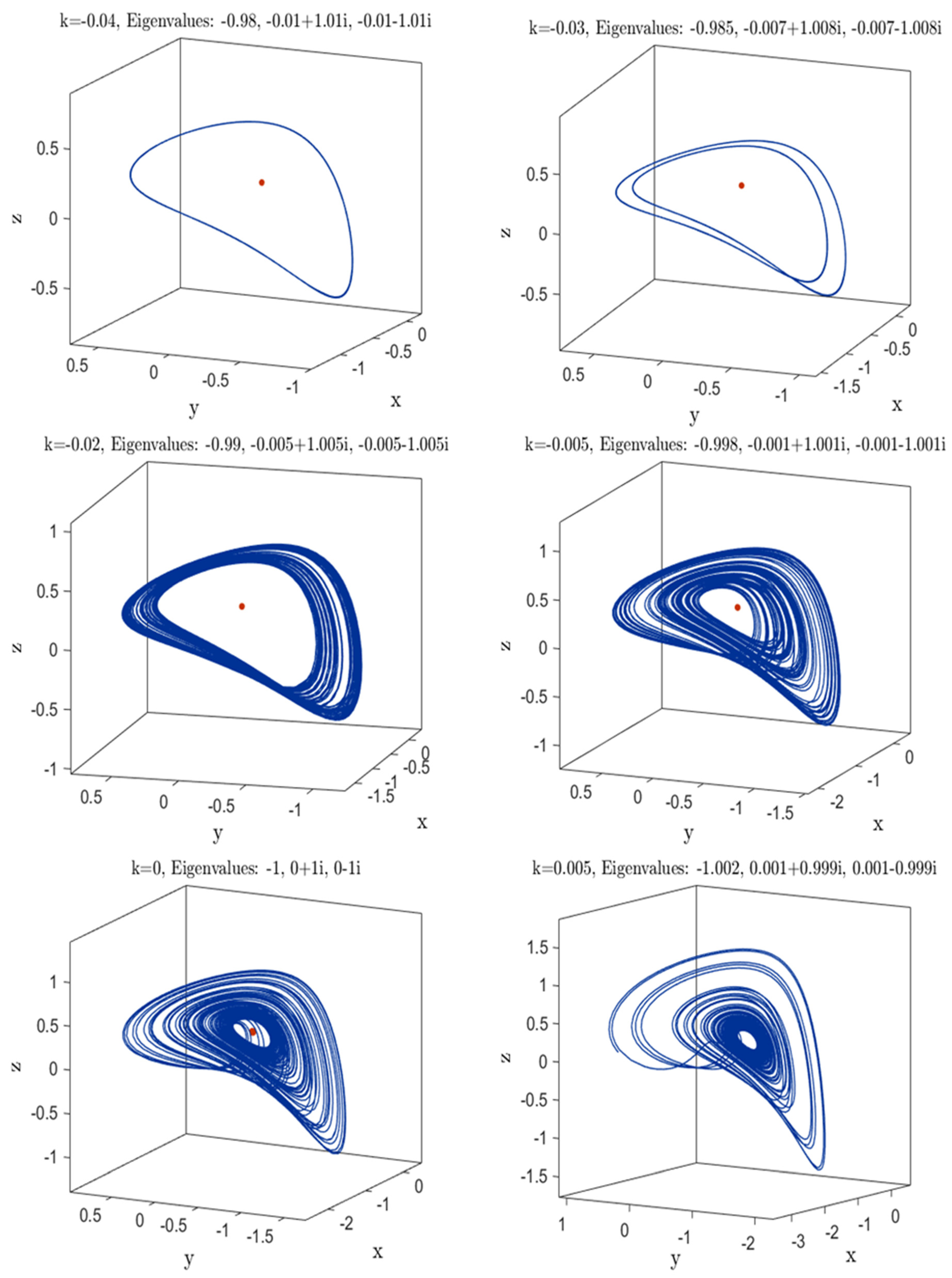
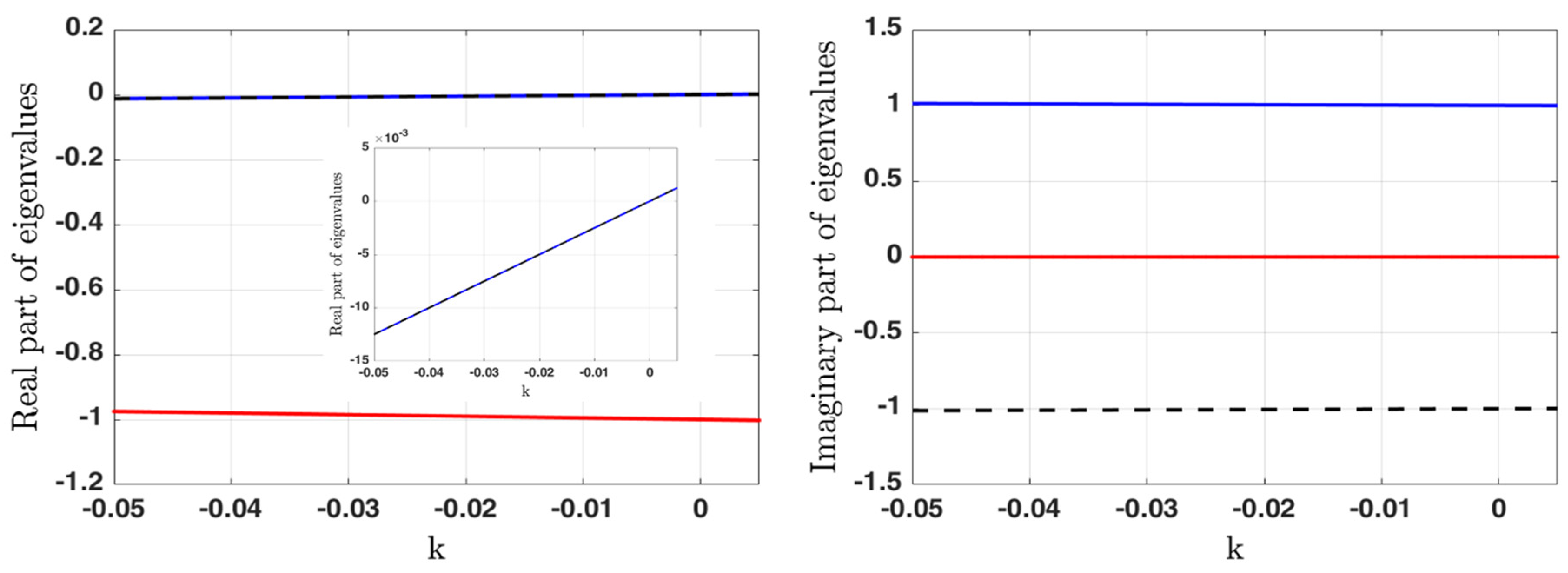
2. Proposed Systems Dynamics

The mathematical model of the new system with only one stable equilibrium is defined as,

$$\begin{array}{c}\dot{x}=y\\ \dot{y}=z\\ \dot{z}=-x-y-z-2.3z^2+xy+k\end{array}$$

(1)

The constant $k$ is a control parameter for the system. To design a new chaotic flow, a specific structure is defended to provide a unique feature. For example, a quadratic jerk system is defined here, and some conditions are computed for the parametric system to have a stable equilibrium. Then, a computer search is applied to find the parameters and initial conditions of a chaotic attractor. Equalizing the left side of the system equations with zero gives one fixed point, E (k, 0, 0). By linearizing System 1 at the equilibrium E, the Jacobian matrix is

$$J=\left[\begin{array}{ccc}0& 1& 0\\ 0& 0& 1\\ -1& k-1& -1\end{array}\right]$$

(2)

Therefore, the characteristic equation at the equilibrium point E is,

$${\lambda }^3+{\lambda }^2+\lambda +1-\lambda k=0$$

(3)

For different k values, solving Equation (3) gives the eigenvalues. Figure 1 shows different dynamics of the system by changing the values of k. On the top of each panel, corresponding eigenvalues are shown. The stability of the fixed-point changes by slightly changing the k parameter. Both periodic and chaotic attractors can be seen by changing the value of the constant controller. Especially for some negative k values, the system has only one stable equilibrium. However, as shown in Figure 1, for k = −0.02 and k = −0.005, the system has a strange attractor. As for these cases, the corresponding fixed points are stable; and the attractors are hidden attractors. Figure 2 shows the real and imaginary parts of eigenvalues of equilibrium point E (k, 0, 0) by changing parameter k. The zoomed view of two larger real parts shows that the equilibrium point is stable in negative k and unstable in positive ones.

Based on the initial condition and specific sets of the control parameter, the system exhibits the coexistence of stable fixed points and chaotic or periodic attractors. In other words, for non-positive k values, by changing initial conditions, the coexistence of one stable equilibrium with a chaotic or periodic attractor is obtained.

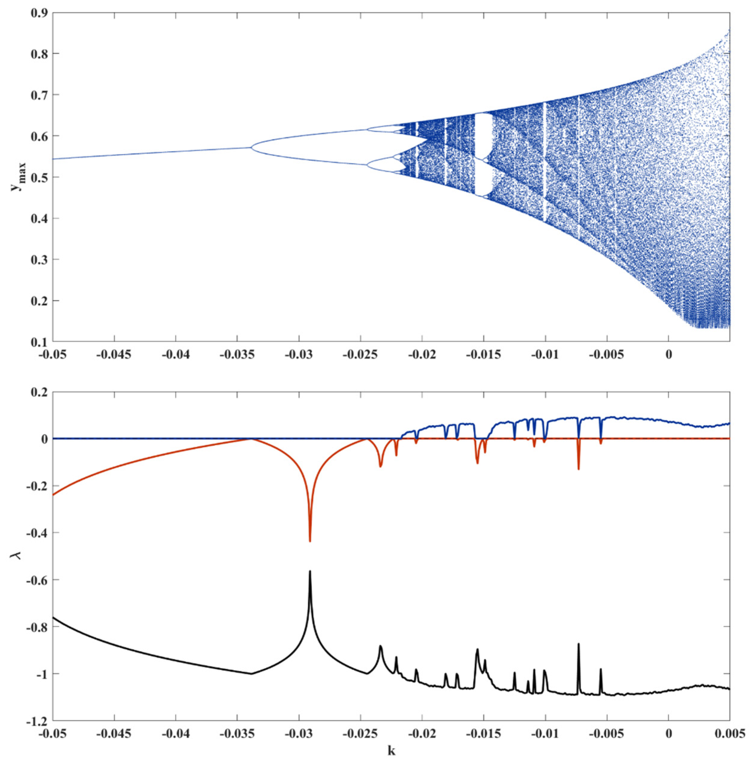
3. Bifurcation Diagram and Lyapunov Exponents

The bifurcation diagram of System (1) based on the k parameter for initial conditions (0, −1, 0) is shown in Figure 3. Figure 3 shows that, based on the control parameter, the system dynamics change from periodic to chaotic. Specifically, period one, period-doubling, and oscillations with higher periods are observed. It should be noted that periodic windows are observed in the bifurcation diagram.

At the bottom of the bifurcation diagrams, the three Lyapunov exponents are plotted with three colors. The maximum Lyapunov exponent is shown in blue. This exponent demonstrates the presence of chaotic regions in the bifurcation diagrams when it is a positive value. When the maximal Lyapunov exponent is zero, the periodic region is proved.

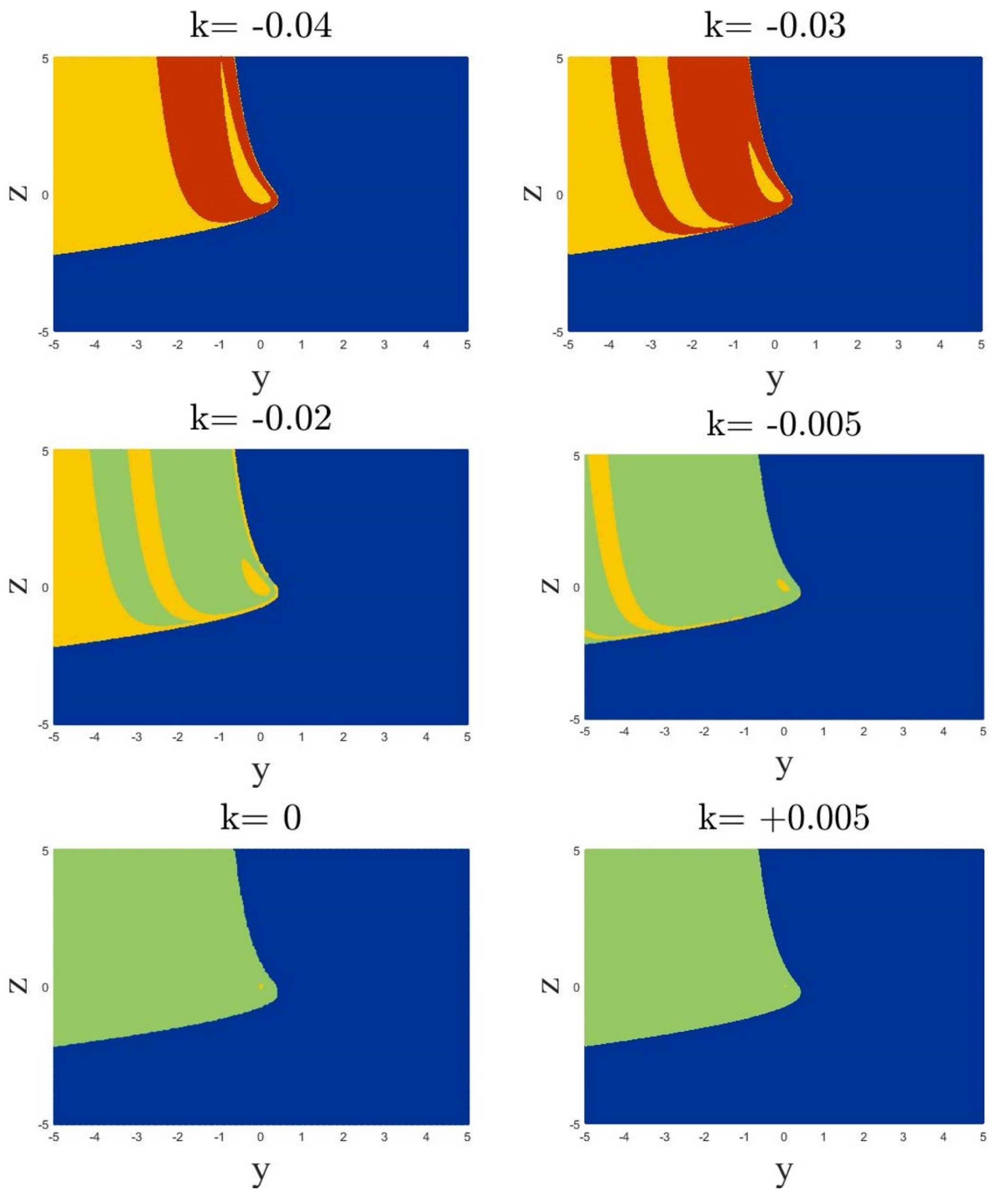
4. Basins of Attractions

The parameter k controls the dynamics of the system to be in the different modes of oscillations. Since the oscillator has an equilibrium point in E (k, 0, 0), different basins of attraction for initial conditions in the plane $x_0=k$ for various k are discussed. The panels of Figure 4 are 2-D cross-sections of 3-D phase space in the y-z plane. Each color shows the steady-state dynamics of the system based on the corresponding initial conditions. The chaotic attractor, periodic attractor, stable fixed point, and unbounded state are shown in green, red, yellow, and blue. For k = −0.04 and k = −0.03, each point on the y-z plane and $x=k$ tends to a periodic attractor, a stable fixed point, or an unbounded oscillation. In both cases, the system’s fixed point is a stable equilibrium; the real parts of all eigenvalues are negative. For k = −0.02 and k = −0.005, the equilibrium is still stable. For some points on the y-z plane, the steady-state dynamics of the system is a stable fixed point, yellow spots. For some other points, the target dynamics of the system are chaotic oscillations, green dots. Since the equilibrium is stable in these cases and is not contained in the basins of the chaotic attractor, the chaotic attractor is classified as a hidden attractor. It is observed that for some k values, including k = 0 and k = +0.005, each point on the basins of attraction has only two destinies, chaotic or unbounded. Since, in this case, the chaotic attractor has an unstable fixed point in its basin of attraction, the chaotic attractor is self-excited. There is no coexistence of the chaotic and periodic attractors for any of the k values; that is why no green spot coexists with red spots in any y-z planes.

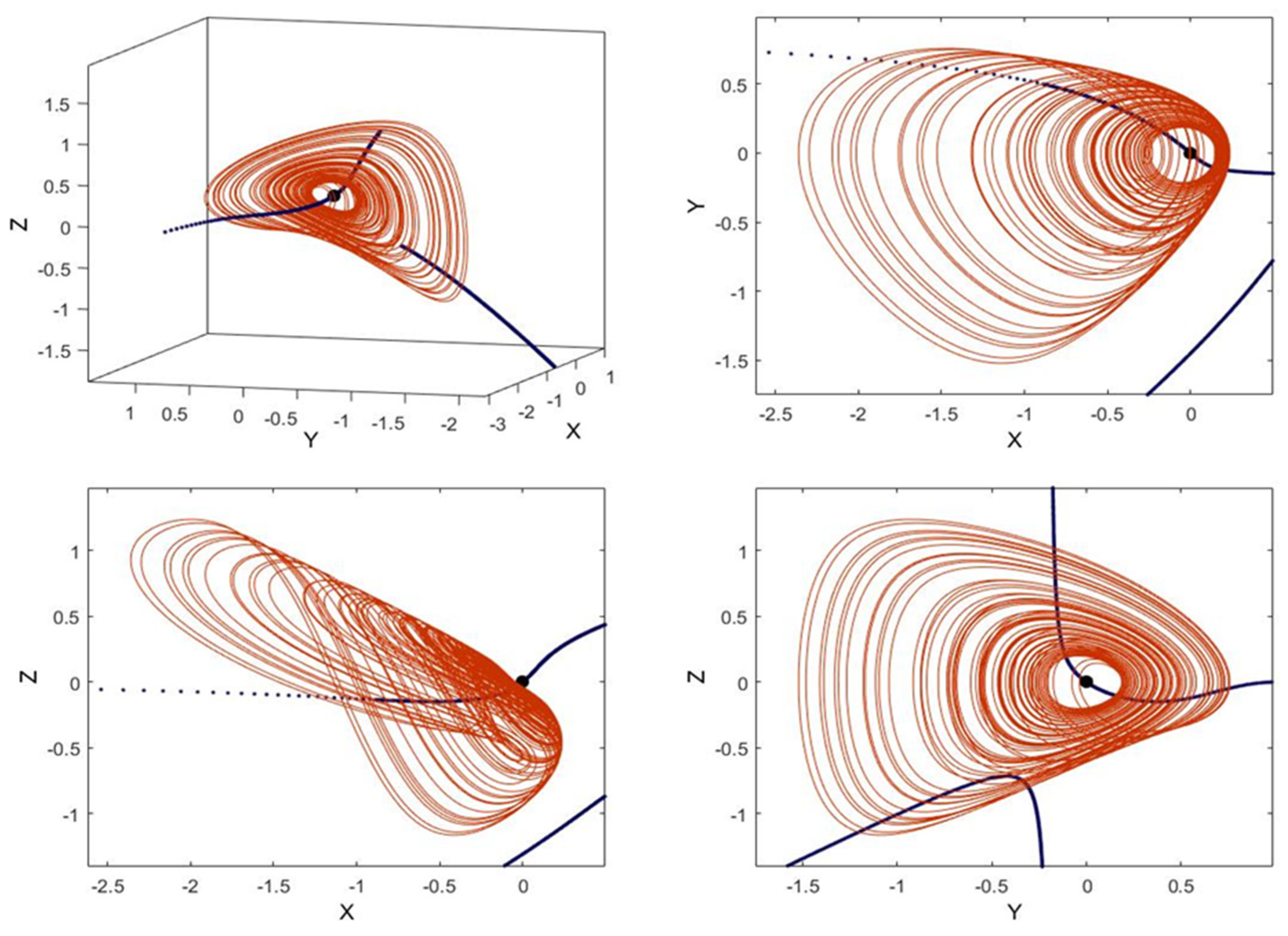
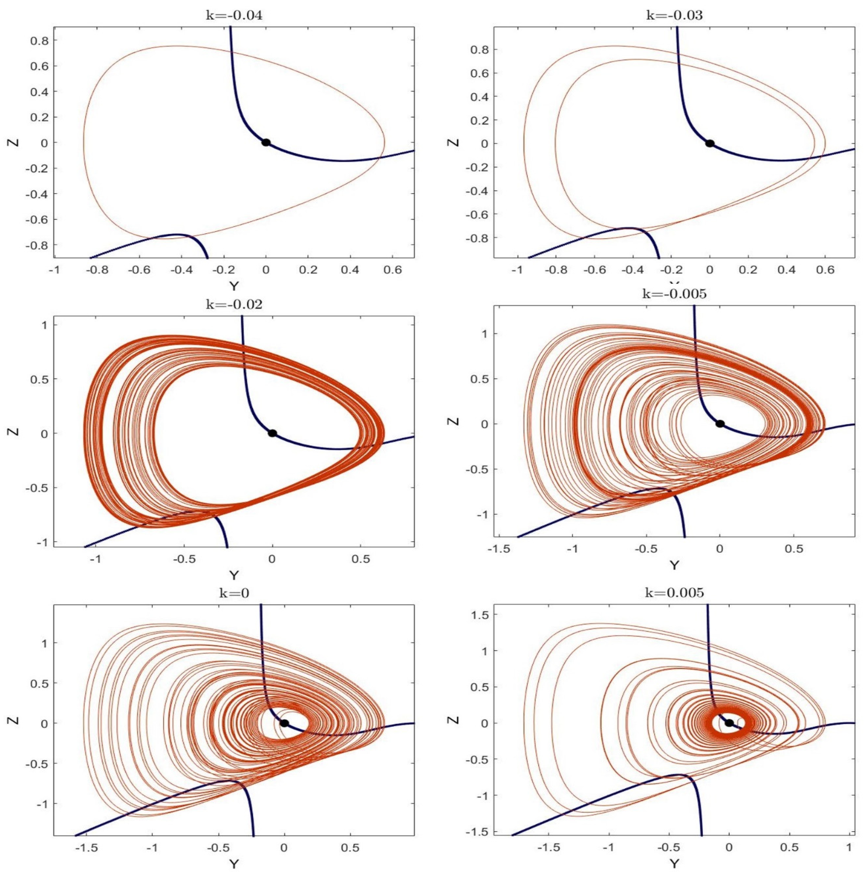
5. Connecting Curves

Connecting curves are one-dimensional invariant sets around which the flow swirls. This one-dimensional set is more informative than zero-dimensional fixed points. Especially in the case of hidden attractors, where there is no corresponding equilibrium, the connecting curve is helpful to understand how the attractor is constructed.

For a dynamical system of differential equations defined as,

$$\overrightarrow{F}={\left(x, y, z\right)}^t$$

(4)

The velocity vector is

$$\frac{d\overrightarrow{F}}{dt}=V\left(t\right)$$

(5)

The acceleration vector is

$$\frac{d\overrightarrow{V}}{dt}=\overrightarrow{\gamma }\left(t\right)=J\overrightarrow{V}$$

(6)

where J is the Jacobian matrix. Then, the connecting curves are sets of point which satisfies the following equation [29],

$$J\overrightarrow{V}=\lambda \overrightarrow{V}$$

(7)

There are points at which the velocity vector is parallel to the acceleration vector, where the principal curvature is zero. Choosing $y$ variable as the phase space coordination and solving Equation (7), other variables are obtained as

$$\begin{array}{c}x=\frac{\frac{23{\lambda }^2{y}^2}{10}+{\lambda }^{2}y+\lambda y+y}{y-1}\\ z=\lambda y\end{array}$$

(8)

Figure 5 shows the connecting curves of System (1) for k = 0 in 3-D space and 2-D planes. The oscillator has a stable equilibrium point in $k\le 0$. Therefore, the attractor of the oscillator is hidden for that interval of the parameter [8]. It should be noted that the connecting curves are independent of attractors, as they are calculated based on the system equations. As shown in Figure 5, the curve passes through the equilibrium; that is why these curves were nominated as connecting curves. It means that the connecting curves connect equilibria since fixed points satisfy Equation (7). As the figure demonstrates, these curves are similar to a skeleton, showing a direction that the attractor evolves around it. Figure 6 shows how the connecting curves depend on parameter k. It was shown that at different k values, the dynamics of the system change from periodic to chaotic, but the structure and direction of evolution remain the same. Accordingly, the connecting curves, which are one-dimensional set of points indicating the evolution of the attractor, do not change majorly when the k value is changed.

6. Conclusions

This study reported a new 3-D chaotic system with only one stable equilibrium. For some control parameters, the system had a strange attractor while its equilibrium was stable. Therefore, the chaotic attractor was hidden. For some other control parameters, its strange attractor was self-excited as its equilibria were unstable. In addition, it was observed that by changing the control parameter, the system exhibits a coexistence of chaotic or periodic oscillations with a stable fixed point. The positive values of the maximal Lyapunov exponent were considered as proof of the chaotic oscillations. Then, the basins of attraction for different control parameters were presented. Finally, the connecting curves of the system were calculated. The connecting curves provided more information than the fixed point, i.e., the curves showed a direction around which the flow swirls and evolves.

References

1. Sprott, J.C. Do we need more chaos examples? Chaos Theory Appl. 2020, 2, 49–51. [Google Scholar]
2. Ma, C.; Mou, J.; Xiong, L.; Banerjee, S.; Liu, T.; Han, X. Dynamical analysis of a new chaotic system: Asymmetric multistability, offset boosting control and circuit realization. Nonlinear Dyn. 2021, 103, 2867–2880. [Google Scholar] [CrossRef]
3. Wang, X.; Chen, G. A chaotic system with only one stable equilibrium. Commun. Nonlinear Sci. Numer. Simul. 2012, 17, 1264–1272. [Google Scholar] [CrossRef] [Green Version]
4. Sprott, J.C. Some simple chaotic flows. Phys. Rev. E 1994, 50, R647. [Google Scholar] [CrossRef]
5. Rajagopal, K.; Duraisamy, P.; Tadesse, G.; Volos, C.; Nazarimehr, F.; Hussain, I. A fractional-order ship power system: Chaos and its dynamical properties. Int. J. Nonlinear Sci. Numer. Simul. 2021. [Google Scholar] [CrossRef]
6. Rajagopal, K.; Shekofteh, Y.; Nazarimehr, F.; Li, C.; Jafari, S. A new chaotic multi-stable hyperjerk system with various types of attractors. Indian J. Phys. 2021, 1–7. [Google Scholar] [CrossRef]
7. Pham, V.-T.; Jafari, S.; Kapitaniak, T.; Volos, C.; Kingni, S.T. Generating a Chaotic System with One Stable Equilibrium. Int. J. Bifurc. Chaos 2017, 27, 1750053. [Google Scholar] [CrossRef]
8. Molaie, M.; Jafari, S.; Sprott, J.C.; Golpayegani, S.M.R.H. Simple chaotic flows with one stable equilibrium. Int. J. Bifurc. Chaos 2013, 23, 1350188. [Google Scholar] [CrossRef]
9. Wei, Z.; Yang, Q. Dynamical analysis of the generalized Sprott C system with only two stable equilibria. Nonlinear Dyn. 2012, 68, 543–554. [Google Scholar] [CrossRef]
10. Wang, X.; Akgul, A.; Cicek, S.; Pham, V.; Hoang, D.V. A chaotic system with two stable equilibrium points: Dynamics, circuit realization and communication application. Int. J. Bifurc. Chaos 2017, 27, 1750130. [Google Scholar] [CrossRef]
11. Tlelo-Cuautle, E.; de la Fraga, L.G.; Pham, V.; Volos, C.; Jafari, S.; de Jesus Quintas-Valles, A. Dynamics, FPGA realization and application of a chaotic system with an infinite number of equilibrium points. Nonlinear Dyn. 2017, 89, 1129–1139. [Google Scholar] [CrossRef]
12. Pham, V.-T.; Jafari, S.; Kapitaniak, T. Constructing a Chaotic System with an Infinite Number of Equilibrium Points. Int. J. Bifurc. Chaos 2016, 26, 1650225. [Google Scholar] [CrossRef]
13. Zhang, S.; Wang, X.; Zeng, Z. A simple no-equilibrium chaotic system with only one signum function for generating multidirectional variable hidden attractors and its hardware implementation. Chaos Interdiscip. J. Nonlinear Sci. 2020, 30, 053129. [Google Scholar] [CrossRef] [PubMed]
14. Chowdhury, S.N.; Ghosh, D. Hidden attractors: A new chaotic system without equilibria. Eur. Phys. J. Spec. Top. 2020, 229, 1299–1308. [Google Scholar] [CrossRef]
15. Lu, H.; Rajagopal, K.; Nazarimehr, F.; Jafari, S. A New Multi-Scroll Megastable Oscillator Based on the Sign Function. Int. J. Bifurc. Chaos 2021, 31, 2150140. [Google Scholar] [CrossRef]
16. Veeman, D.; Natiq, H.; Al-Saidi, N.M.G.; Rajagopal, K.; Jafari, S.; Hussain, I. A New Megastable Chaotic Oscillator with Blinking Oscillation terms. Complexity 2021, 2021, 5518633. [Google Scholar] [CrossRef]
17. Li, X.; Mou, J.; Xiong, L.; Wang, Z.; Xu, J. Fractional-order double-ring erbium-doped fiber laser chaotic system and its application on image encryption. Opt. Laser Technol. 2021, 140, 107074. [Google Scholar] [CrossRef]
18. Karthikeyan, A.; ÇİÇEK, S.; Rajagopal, K.; Duraisamy, P.; Srinivasan, A. New hyperchaotic system with single nonlinearity, its electronic circuit and encryption design based on current conveyor. Turk. J. Electr. Eng. Comput. Sci. 2021, 29, 1692–1705. [Google Scholar] [CrossRef]
19. Cang, S.; Kang, Z.; Wang, Z. Pseudo-random number generator based on a generalized conservative Sprott-A system. Nonlinear Dyn. 2021, 1–18. [Google Scholar] [CrossRef]
20. Wang, N.; Zhang, G.; Kuznetsov, N.V.; Baoe, H. Hidden attractors and multistability in a modified Chua’s circuit. Commun. Nonlinear Sci. Numer. Simul. 2021, 92, 105494. [Google Scholar] [CrossRef]
21. Deng, Q.; Wang, C.; Yang, L. Four-wing hidden attractors with one stable equilibrium point. Int. J. Bifurc. Chaos 2020, 30, 2050086. [Google Scholar] [CrossRef]
22. Jafari, S.; Sprott, J.; Nazarimehr, F. Recent new examples of hidden attractors. Eur. Phys. J. Spec. Top. 2015, 224, 1469–1476. [Google Scholar] [CrossRef]
23. Dudkowski, D.; Jafari, S.; Kapitaniak, T.; Kuznetsov, N.V.; Leonov, G.A.; Prasad, A. Hidden attractors in dynamical systems. Phys. Rep. 2016, 637, 1–50. [Google Scholar] [CrossRef]
24. Leonov, G.; Kuznetsov, N.; Vagaitsev, V. Localization of hidden Chua’s attractors. Phys. Lett. A 2011, 375, 2230–2233. [Google Scholar] [CrossRef]
25. Kuznetsov, N.V. Hidden attractors in fundamental problems and engineering models: A short survey. In AETA 2015: Recent Advances in Electrical Engineering and Related Sciences; Springer: Berlin/Heidelberg, Germany, 2016; pp. 13–25. [Google Scholar]
26. Dudkowski, D.; Prasad, A.; Kapitaniak, T. Perpetual Points: New Tool for Localization of Coexisting Attractors in Dynamical Systems. Int. J. Bifurc. Chaos 2017, 27, 1750063. [Google Scholar] [CrossRef] [Green Version]
27. Nazarimehr, F.; Saedi, B.; Jafari, S.; Sprott, J.C. Are perpetual points sufficient for locating hidden attractors? Int. J. Bifurc. Chaos 2017, 27, 1750037. [Google Scholar] [CrossRef]
28. Roth, M.; Peikert, R. A higher-order method for finding vortex core lines. In Proceedings of the Visualization’98 (Cat. No. 98CB36276), Research Triangle Park, NC, USA, 18–23 October 1998. [Google Scholar]
29. Gilmore, R.; Ginoux, J.M.; Jones, T.; Letellier, C.; Freitas, U.S. Connecting curves for dynamical systems. J. Phys. A Math. Theor. 2010, 43, 255101. [Google Scholar] [CrossRef]
Figure 1. Attractors of System (1) with two different initial conditions. For the initial condition (0, −1, 0), the system tends to have chaotic or periodic attractors dependent on the parameter k. For non−positive k values, the initial condition (−0.01, 0.01, 0.01) tends to the red dot equilibrium. At the top of each panel, the corresponding eigenvalues are presented.
Mathematics 09 03217 g001
Figure 2. The real and imaginary parts of the three eigenvalues with different colors. Moreover, the zoomed view of two larger values of real parts is presented.
Mathematics 09 03217 g002
Figure 3. The bifurcation diagrams of System (1) versus k parameter and corresponding Lyapunov exponents for initial conditions (0, −1, 0).
Mathematics 09 03217 g003
Figure 4. 2−D cross−sections of basins of attractions of System (1). Initial conditions belonging to blue regions lead to unbounded oscillation. The yellow part contains initial conditions that show the system to its stable equilibrium. Periodic and chaotic attractors emerge from the red and green points in the y-z plane. The initial condition for the x variable is selected as x = k for all panels.
Mathematics 09 03217 g004
Figure 5. Connecting curves of System (1) in k = 0. It is observed that the connecting curves are skeleton−like curves around which the flow evolves. Additionally, it is obtained that the curve passes through the fixed point.
Mathematics 09 03217 g005
Figure 6. The connecting curves of System (1) for different k values and associated attractors. It is shown that the connecting curves represent the structure of the attractors, and since the structure of attractors did not change majorly, with different k values, the curves remain approximately unchanged.
Mathematics 09 03217 g006
Publisher’s Note: MDPI stays neutral with regard to jurisdictional claims in published maps and institutional affiliations.