Roots of Characteristic Polynomial Sequences in Iterative Block Cyclic Reductions

Abstract

The block cyclic reduction method is a finite-step direct method used for solving linear systems with block tridiagonal coefficient matrices. It iteratively uses transformations to reduce the number of non-zero blocks in coefficient matrices. With repeated block cyclic reductions, non-zero off-diagonal blocks in coefficient matrices incrementally leave the diagonal blocks and eventually vanish after a finite number of block cyclic reductions. In this paper, we focus on the roots of characteristic polynomials of coefficient matrices that are repeatedly transformed by block cyclic reductions. We regard each block cyclic reduction as a composition of two types of matrix transformations, and then attempt to examine changes in the existence range of roots. This is a block extension of the idea presented in our previous papers on simple cyclic reductions. The property that the roots are not very scattered is a key to accurately solve linear systems in floating-point arithmetic. We clarify that block cyclic reductions do not disperse roots, but rather narrow their distribution, if the original coefficient matrix is symmetric positive or negative definite.

1. Introduction

Solving systems of linear equations is one of the most important subjects in numerical linear algebra. In particular, applied mathematics and engineering often require the solution of linear systems with tridiagonal coefficient matrices. Solving tridiagonal linear systems generally involves finding N-dimensional vectors $\mathit{x}$, such that $A\mathit{x}=\mathit{b}$ for given N-by-N tridiagonal matrices A and N-dimensional vectors $\mathit{b}$. The cyclic reduction method is a finite-step direct method for computing solutions $\mathit{x}$ [1,2]. The cyclic reduction method first transforms tridiagonal coefficient matrices A to pentadiagonal matrices with all subdiagonal (and superdiagonal) entries equal to 0. The right vectors $\mathit{b}$ are, of course, simultaneously changed. Two non-zero off-diagonals of the coefficient matrices gradually leave the diagonals in the iterative cyclic reductions, with the coefficient matrices eventually being reduced to diagonal matrices. Error analysis of the cyclic reduction method has been reported in [3], and a variant of the cyclic reduction method has been also presented, for example, in [4]. The stride reduction method is a generalization of the cyclic reduction method that can solve problems where A are M-tridiagonal matrices, M is the bandwidth, and there are two non-zero off-diagonals consisting of $(1,M+1)$, $(2,M+2)$, …, $(N-M-1,N)$ and the $(M+1,1)$, $(M+2,2)$, …, $(N,N-M-1)$ entries [5]. Each stride reduction, including cyclic reduction, narrows the distribution of the roots of characteristic polynomials associated with the coefficient matrices if A are symmetric positive definite [6,7]. This is a desirable property that does not increase the difficulty of solving systems of linear systems.

Here, we consider positive integers $N_1,N_2,\cdots ,N_m$ satisfying $N=N_1+N_2+\cdots +N_m$. The cyclic reduction method is extended to solve a problem where coefficient matrices $A\in {\mathbb{R}}^{N\times N}$ are block tridiagonal matrices [2,8] expressed using m square matrices $D_1\in {\mathbb{R}}^{N_1\times N_1}$, $D_2\in {\mathbb{R}}^{N_2\times N_2}$, …, $D_m\in {\mathbb{R}}^{N_m\times N_m}$ and $2m-2$ rectangular matrices $E_1\in {\mathbb{R}}^{N_1\times N_2}$, $E_2\in {\mathbb{R}}^{N_2\times N_3}$, …, $E_{m-1}\in {\mathbb{R}}^{N_{m-1}\times N_m}$ and $F_1\in {\mathbb{R}}^{N_2\times N_1}$, $F_2\in {\mathbb{R}}^{N_3\times N_2}$, …, $F_{m-1}\in {\mathbb{R}}^{N_m\times N_{m-1}}$ as:

$$\begin{array}{c}\hfill A:=\left(\begin{array}{ccc}{D}_1& E_1& \\ F_1& D_2& \ddots \\ & \ddots & \ddots & E_{m-1}\\ & & F_{m-1}& D_m\end{array}\right).\end{array}$$

(1)

A block tridiagonal matrix can be regarded as a block matrix obtained by replacing the diagonal entries in a tridiagonal matrix with square matrices and the subdiagonal entries with rectangular matrices. This extended method is called the block cyclic reduction method. The forward stability of iterative block cyclic reductions has been discussed in [9], but changes in roots of characteristic polynomials of coefficient matrices have not been studied. Block cyclic reductions do not work well in floating point arithmetic if they greatly disperse the roots. Thus, the main purpose of this paper is to clarify whether block cyclic reductions narrow the root distribution like stride reductions.

The remainder of this paper is organized as follows. Section 2 briefly explains the block cyclic reduction method used for solving block tridiagonal linear systems. Section 3 shows that block M-tridiagonal matrices can be transformed to block tridiagonal (1-tridiagonal) matrices without changing the eigenvalues. Then, we interpret the transformation from M-tridiagonal matrices to $2M$-tridiagonal matrices in the block cyclic reduction as a composite transformation of the block tridiagonalization, its inverse, and the transformation from block tridiagonal to block 2-tridiagonal matrices. In Section 4, we find the relationship between the inverses of block tridiagonal matrices and those of block 2-tridiagonal matrices. Section 5 looks at the roots of characteristic polynomials of coefficient matrices transformed by block cyclic reductions compared with those of original coefficient matrices A in cases where A are block tridiagonal and symmetric positive definite or negative definite. Section 6 gives two numerical examples for observing coefficient matrices and the roots of their characteristic polynomials appearing in iterative block cyclic reductions. Section 7 concludes the paper.

2. Block Cyclic Reduction

In this section, we briefly explain the block cyclic reduction method used for solving linear systems with block tridiagonal coefficient matrices.

We consider the following N-by-N block-band matrix given using m square matrices $D_1^{\left(M\right)}\in {\mathbb{R}}^{N_1\times N_1}$, $D_2^{\left(M\right)}\in {\mathbb{R}}^{N_2\times N_2}$, ⋯, $D_m^{\left(M\right)}\in {\mathbb{R}}^{N_m\times N_m}$ and $2(m-M)$ rectangular matrices $E_1^{\left(M\right)}\in {\mathbb{R}}^{N_1\times N_{1+M}}$, $E_2^{\left(M\right)}\in {\mathbb{R}}^{N_2\times N_{2+M}}$, ⋯, $E_{m-M}^{\left(M\right)}\in {\mathbb{R}}^{N_{m-M}\times N_m}$ and $F_1^{\left(M\right)}\in {\mathbb{R}}^{N_{1+M}\times N_1}$, $F_2^{\left(M\right)}\in {\mathbb{R}}^{N_{2+M}\times N_2}$, ⋯, $F_{m-M}^{\left(M\right)}\in {\mathbb{R}}^{N_m\times N_{m-M}}$ as:

$$\begin{array}{c}\hfill A^{\left(M\right)}:=\left(\begin{array}{ccc}{D}_1^{\left(M\right)}& & E_1^{\left(M\right)}\\ & \ddots & & \ddots \\ F_1^{\left(M\right)}& & D_{1+M}^{\left(M\right)}& & \ddots \\ & \ddots & & \ddots & & \ddots & \\ & & \ddots & & D_{m-M}^{\left(M\right)}& & E_{m-M}^{\left(M\right)}\\ & & & \ddots & & \ddots \\ & & & & F_{m-M}^{\left(M\right)}& & D_m^{\left(M\right)}\end{array}\right),\end{array}$$

(2)

where the superscript in parentheses appearing in $A^{\left(M\right)}$ specifies the position of non-zero off-diagonal bands $E_i^{\left(M\right)}$ and $F_i^{\left(M\right)}$. If $D_i^{\left(M\right)}$, $E_i^{\left(M\right)}$, and $F_i^{\left(M\right)}$ are all 1-by-1 matrices for every i, then $A^{\left(M\right)}$ is the M-tridiagonal matrix [6] and $D_i^{\left(M\right)}$, $E_i^{\left(M\right)}$, and $F_i^{\left(M\right)}$ are the $(i,i)$, $(i,i+M)$, and $(i+M,i)$ entries of $A^{\left(M\right)}$, respectively. Thus, we hereinafter refer to $A^{\left(M\right)}$ as the block M-tridiagonal matrix and $D_i^{\left(M\right)}$, $E_i^{\left(M\right)}$, and $F_i^{\left(M\right)}$ as the $(i,i)$, $(i,i+M)$, and $(i+M,i)$ blocks of $A^{\left(M\right)}$, respectively. Note that block 1-tridiagonal matrices are the usual block tridiagonal matrices. In the case where $D_i^{\left(M\right)}$, $E_i^{\left(M\right)}$, and $F_i^{\left(M\right)}$ are not 1-by-1 matrices, we must pay attention to the number of rows and columns of $D_i^{\left(M\right)}$, $E_i^{\left(M\right)}$, and $F_i^{\left(M\right)}$. For example, we can compute the matrix product $D_1^{\left(M\right)}{E}_1^{\left(M\right)}$ but cannot define $E_1^{\left(M\right)}{D}_1^{\left(M\right)}$ if $N_1\ne N_{1+M}$, unlike in the case where $D_i^{\left(M\right)}$, $E_i^{\left(M\right)}$, and $F_i^{\left(M\right)}$ are all 1-by-1 matrices.

We hereinafter consider the case where $D_i^{\left(M\right)}$ are all nonsingular. Here, we prepare an N-by-N block M-tridiagonal matrix involving non-zero blocks $D_i^{\left(M\right)}$, $E_i^{\left(M\right)}$, and $F_i^{\left(M\right)}$:

$$\begin{array}{cc}\hfill & T^{\left(M\right)}:=\hfill \\ \hfill & \left(\begin{array}{ccc}{I}_1& & -E_1^{\left(M\right)}{\left(D_{1+M}^{\left(M\right)}\right)}^{-1}\\ & \ddots & & \ddots \\ -F_1^{\left(M\right)}{\left(D_1^{\left(M\right)}\right)}^{-1}& & I_{1+M}& & \ddots \\ & \ddots & & \ddots & & \ddots \\ & & \ddots & & I_{m-M}& & -E_{m-M}^{\left(M\right)}{\left(D_m^{\left(M\right)}\right)}^{-1}\\ & & & \ddots & & \ddots \\ & & & & -F_{m-M}^{\left(M\right)}{\left(D_{m-M}^{\left(M\right)}\right)}^{-1}& & I_m\end{array}\right),\hfill \end{array}$$

(3)

where $I_i$ are the $N_i$-by-$N_i$ identity matrices. The number of rows and columns of $I_i$, $-E_i^{\left(M\right)}{\left(D_{i+M}^{\left(M\right)}\right)}^{-1}$, and $-F_i^{\left(M\right)}{\left(D_i^{\left(M\right)}\right)}^{-1}$ coincide with those of $D_i^{\left(M\right)}$, $E_i^{\left(M\right)}$, and $F_i^{\left(M\right)}$, respectively. In other words, $T^{\left(M\right)}$ has the same block structure as $A^{\left(M\right)}$. Then, we can easily observe that the $(i,i+M)$ and $(i+M,i)$ blocks are all zero and the $(i,i+2M)$ and $(i+2M,i)$ blocks of $T^{\left(M\right)}{A}^{\left(M\right)}$ are all non-zero, meaning that $T^{\left(M\right)}{A}^{\left(M\right)}$ becomes an N-by-N block $2M$-tridiagonal matrix $A^{\left(2M\right)}$, The non-zero blocks $D_i^{\left(2M\right)}$, $E_i^{\left(2M\right)}$, and $F_i^{\left(2M\right)}$ appearing in the $(i,i)$, $(i,i+2M)$, and $(i+2M,i)$ blocks are also expressed using $D_i^{\left(M\right)}$, $E_i^{\left(M\right)}$, and $F_i^{\left(M\right)}$ as:

$$\begin{array}{c}\hfill \left\{\begin{array}{c}{D}_i^{\left(2M\right)}:=D_i^{\left(M\right)}-E_i^{\left(M\right)}{\left(D_{i+M}^{\left(M\right)}\right)}^{-1}{F}_i^{\left(M\right)},i=1,2,\cdots ,M,\hfill \\ D_i^{\left(2M\right)}:=D_i^{\left(M\right)}-F_{i-M}^{\left(M\right)}{\left(D_{i-M}^{\left(M\right)}\right)}^{-1}{E}_{i-M}^{\left(M\right)}-E_i^{\left(M\right)}{\left(D_{i+M}^{\left(M\right)}\right)}^{-1}{F}_i^{\left(M\right)},i=M+1,\cdots ,m-M,\hfill \\ D_i^{\left(2M\right)}:=D_i^{\left(M\right)}-F_{i-M}^{\left(M\right)}{\left(D_{i-M}^{\left(M\right)}\right)}^{-1}{E}_{i-M}^{\left(M\right)},i=m-M+1,m-M+2,\cdots ,m,\hfill \\ E_i^{\left(2M\right)}:=-E_i^{\left(M\right)}{\left(D_{i+M}^{\left(M\right)}\right)}^{-1}{E}_{i+M}^{\left(M\right)},i=1,2,\cdots ,m-2M,\hfill \\ F_i^{\left(2M\right)}:=-F_{i+M}^{\left(M\right)}{\left(D_{i+M}^{\left(M\right)}\right)}^{-1}{F}_i^{\left(M\right)},i=1,2,\cdots ,m-2M.\hfill \end{array}\right.\end{array}$$

(4)

Thus, by multiplying the block M-tridiagonal linear system $A^{\left(M\right)}\mathit{x}={\mathit{b}}^{\left(M\right)}$ by $T^{\left(M\right)}$ from the left on both sides, we transform it to the block $2M$-tridiagonal linear system $A^{\left(2M\right)}\mathit{x}={\mathit{b}}^{\left(2M\right)}$, where ${\mathit{b}}^{\left(2M\right)}:=T^{\left(M\right)}{\mathit{b}}^{\left(M\right)}$. This transformation is the block cyclic reduction [2]. We can again apply the block cyclic reduction to the block $2M$-tridiagonal linear system $A^{\left(2M\right)}\mathit{x}={\mathit{b}}^{\left(2M\right)}$ if the diagonal blocks $D_i^{\left(2M\right)}$ in the block $2M$-tridiagonal matrix $A^{\left(2M\right)}$ are all nonsingular. The iterative block cyclic reductions therefore cause non-zero off-diagonal blocks to gradually leave the diagonal blocks, eventually generating linear systems with block diagonal matrices.

3. Composite Transformation

In this section, we first show that block M-tridiagonal matrices can be transformed into block tridiagonal (1-tridiagonal) matrices while preserving the eigenvalues. Next, we consider the transformation from the block M-tridiagonal matrix $A^{\left(M\right)}$ to the block $2M$-tridiagonal matrix $A^{\left(2M\right)}$ in terms of the transformation from the block tridiagonal (1-tridiagonal) matrix to the block 2-tridiagonal matrix with two similarity transformations.

We consider N-by-$N_i$ matrices:

$$\begin{array}{c}\hfill P_i:=\left(\begin{array}{c}O\\ ⋮\\ O\\ I_i\\ O\\ ⋮\\ O\end{array}\right)\begin{array}{c}1\mathrm{st}\mathrm{block}\hfill \\ \\ (i-1)\mathrm{th}\mathrm{block}\hfill \\ i\mathrm{th}\mathrm{block}\hfill \\ (i+1)\mathrm{th}\mathrm{block}\hfill \\ \\ m\mathrm{th}\mathrm{block}\hfill \end{array},i=1,2,\cdots ,m,\end{array}$$

(5)

where O denotes the zero matrix, whose entries are all 0, and the number of rows in the 1st, 2nd, ⋯, mth blocks are equal to those in $D_1^{\left(M\right)}$, $D_2^{\left(M\right)}$, ⋯, $D_m^{\left(M\right)}$, respectively. Then, it is obvious that $A^{\left(M\right)}{P}_1$$\in {\mathbb{R}}^{N\times N_1}$, $A^{\left(M\right)}{P}_2\in {\mathbb{R}}^{N\times N_2}$, ⋯, $A^{\left(M\right)}{P}_m\in {\mathbb{R}}^{N\times N_m}$ become the 1st, 2nd, ⋯, mth block-columns of $A^{\left(M\right)}$, respectively. Furthermore, for $i=1,2,\cdots ,m$, it is observed that $P_1^{\top }\left(A^{\left(M\right)}{P}_i\right)\in {\mathbb{R}}^{N_1\times N_i}$, $P_2^{\top }\left(A^{\left(M\right)}{P}_i\right)\in {\mathbb{R}}^{N_2\times N_i}$, ⋯, $P_m^{\top }\left(A^{\left(M\right)}{P}_i\right)\in {\mathbb{R}}^{N_m\times N_i}$ coincide with the 1st, 2nd, ⋯, mth block-rows of $A^{\left(M\right)}{P}_i$, respectively. Thus, we see that $P_j^{\top }{A}^{\left(M\right)}{P}_i$ are the $(j,i)$ blocks of $A^{\left(M\right)}$ for $i,j=1,2,\cdots ,m$—namely:

$$\begin{array}{cc}\hfill & P_j^{\top }{A}^{\left(M\right)}{P}_i=\left\{\begin{array}{cc}{E}_i^{\left(M\right)},\hfill & j=i-M,\hfill \\ D_i^{\left(M\right)},\hfill & j=i,\hfill \\ F_i^{\left(M\right)},\hfill & j=i+M,\hfill \\ O,\hfill & otherwise.\hfill \end{array}\right.\hfill \end{array}$$

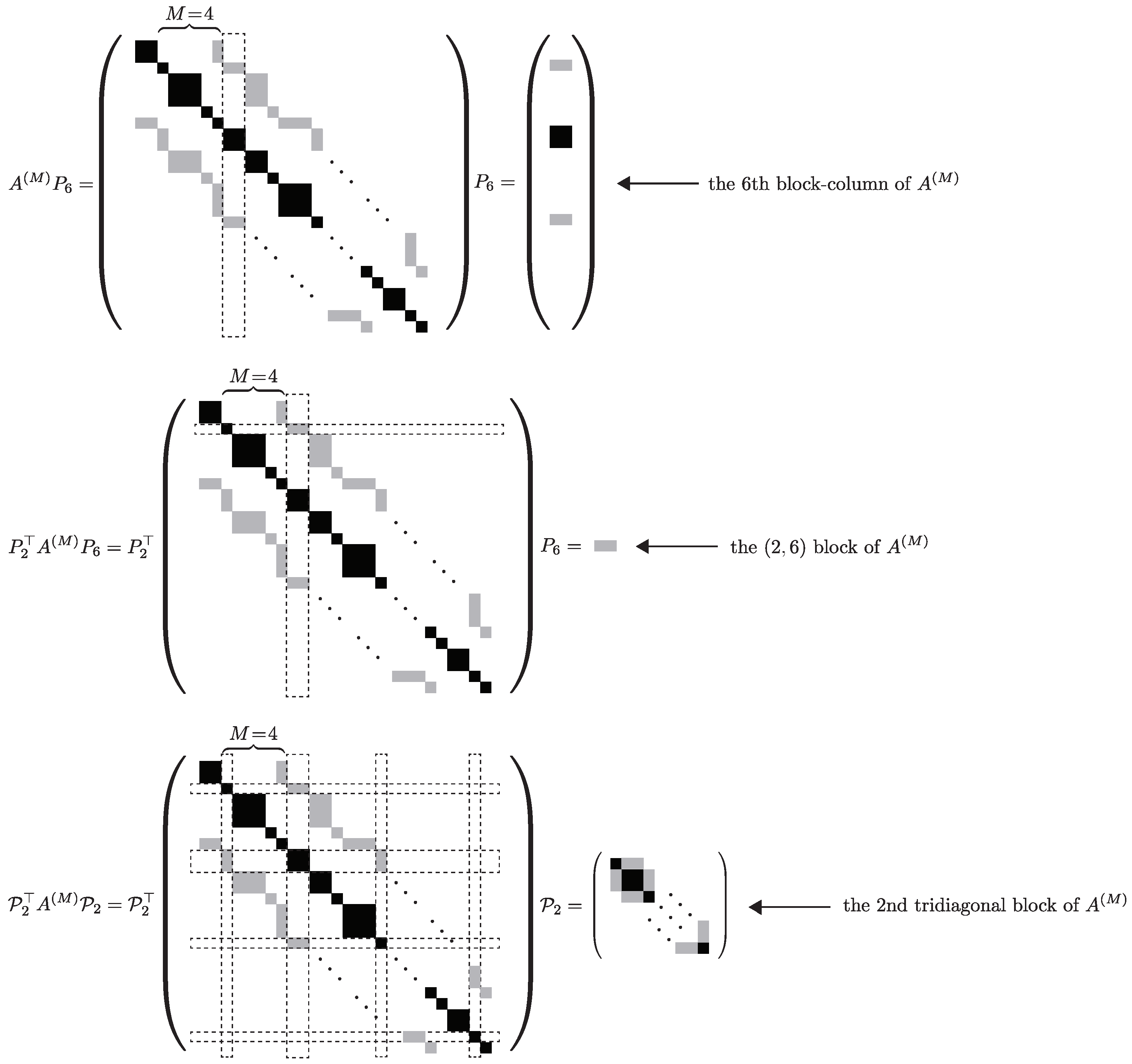
Here, we introduce $N\times (N_i+N_{i+M}+\cdots +N_{i+qM})$ matrices ${\mathcal{P}}_i:=(P_i,P_{i+M},\cdots ,$$P_{i+qM})$ for $i=1,2,\cdots ,r$, where q and r are the quotient and the remainder after the division of m by M, respectively. Then, it follows that:

$$\begin{array}{cc}\hfill & {\mathcal{P}}_i^{\top }{A}^{\left(M\right)}{P}_i=\left(\begin{array}{c}{D}_i^{\left(M\right)}\\ F_i^{\left(M\right)}\\ O\\ ⋮\\ O\end{array}\right)\in {\mathbb{R}}^{(N_i+N_{i+M}+\cdots +N_{i+qM})\times N_i},i=1,2,\cdots ,r.\hfill \\ \hfill & {\mathcal{P}}_i^{\top }{A}^{\left(M\right)}{P}_{i+kM}=\left(\begin{array}{c}O\\ ⋮\\ O\\ E_{i+(k-1)M}^{\left(M\right)}\\ D_{i+kM}^{\left(M\right)}\\ F_{i+kM}^{\left(M\right)}\\ O\\ ⋮\\ O\end{array}\right)\in {\mathbb{R}}^{(N_i+N_{i+M}+\cdots +N_{i+qM})\times N_{i+kM}},\hfill \\ \hfill & i=1,2,\cdots ,r,k=1,2,\cdots ,q-1,\hfill \\ \hfill & {\mathcal{P}}_i^{\top }{A}^{\left(M\right)}{P}_{i+qM}=\left(\begin{array}{c}O\\ ⋮\\ O\\ E_{i+(q-1)M}^{\left(M\right)}\\ D_{i+qM}^{\left(M\right)}\end{array}\right)\in {\mathbb{R}}^{(N_i+N_{i+M}+\cdots +N_{i+qM})\times N_{i+qM}},i=1,2,\cdots ,r.\hfill \end{array}$$

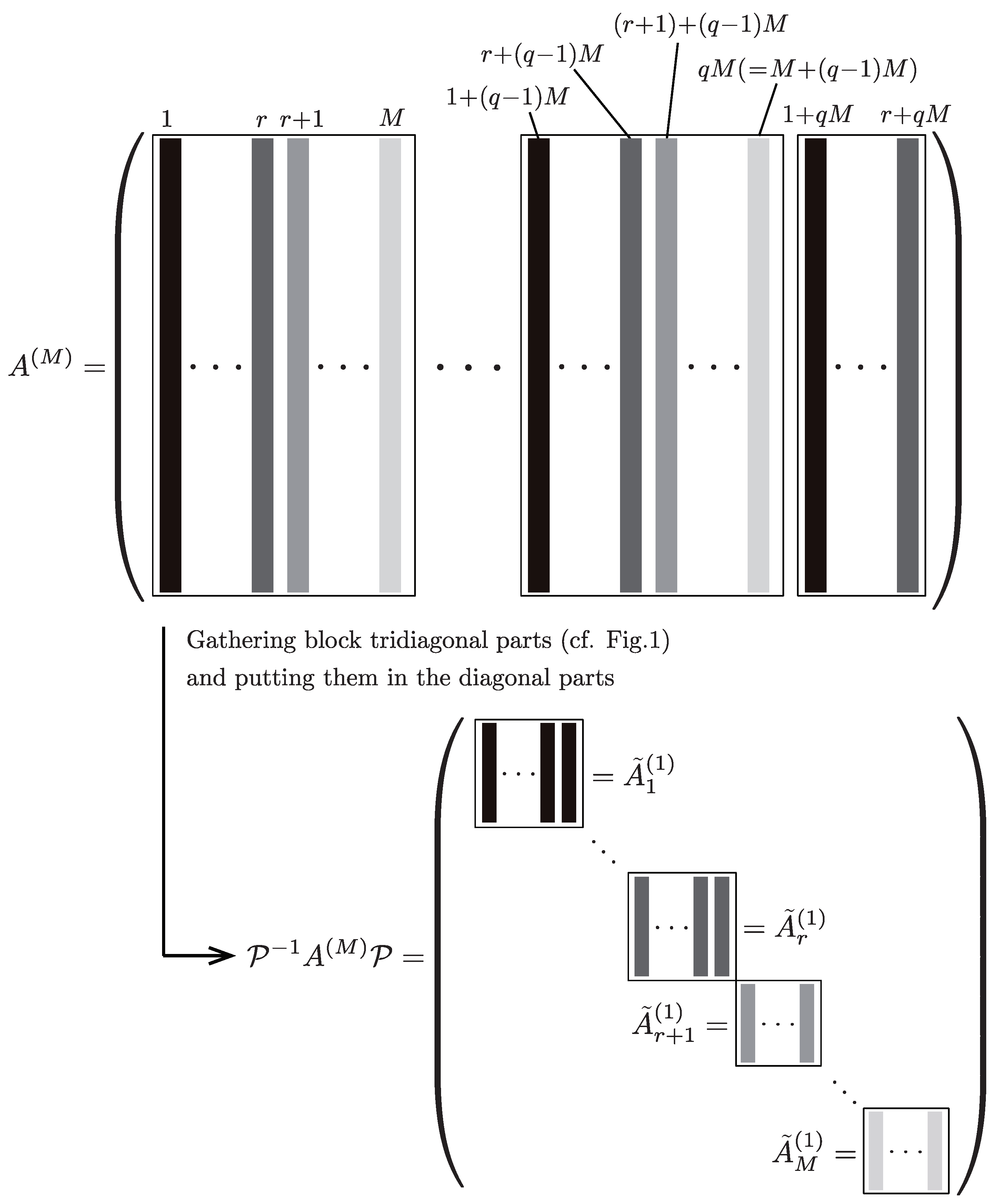
Thus, by gathering these, we can derive:

$$\begin{array}{cc}\hfill {\mathcal{P}}_i^{\top }{A}^{\left(M\right)}{\mathcal{P}}_i=& \left(\begin{array}{cc}{D}_i^{\left(M\right)}& E_i^{\left(M\right)}\\ F_i^{\left(M\right)}& D_{i+M}^{\left(M\right)}& \ddots \\ & \ddots & \ddots & E_{i+(q-1)M}^{\left(M\right)}\\ & & F_{i+(q-1)M}^{\left(M\right)}& D_{i+qM}^{\left(M\right)}\end{array}\right)\hfill \\ \hfill & \in {\mathbb{R}}^{(N_i+N_{i+M}+\cdots +N_{i+qM})\times (N_i+N_{i+M}+\cdots +N_{i+qM})},i=1,2,\cdots ,r.\hfill \end{array}$$

(6)

Similarly, by letting ${\mathcal{P}}_i:=(P_i,P_{i+M},\cdots ,P_{i+(q-1)M})\in {\mathbb{R}}^{N\times (N_i+N_{i+M}+\cdots +N_{i+(q-1)M})}$ for $i=r+1,r+2,\cdots ,M$, we obtain:

$$\begin{array}{cc}\hfill {\mathcal{P}}_i^{\top }{A}^{\left(M\right)}{\mathcal{P}}_i=& \left(\begin{array}{cc}{D}_i^{\left(M\right)}& E_i^{\left(M\right)}\\ F_i^{\left(M\right)}& D_{i+M}^{\left(M\right)}& \ddots \\ & \ddots & \ddots & E_{i+(q-2)M}^{\left(M\right)}\\ & & F_{i+(q-2)M}^{\left(M\right)}& D_{i+(q-1)M}^{\left(M\right)}\end{array}\right)\hfill \\ \hfill & \in {\mathbb{R}}^{(N_i+N_{i+M}+\cdots +N_{i+(q-1)M})\times (N_i+N_{i+M}+\cdots +N_{i+(q-1)M})},\hfill \\ \hfill & \phantom{\in }i=r+1,r+2,\cdots ,M.\hfill \end{array}$$

(7)

See, also, Figure 1 for an auxiliary example of gathering a block tridiagonal part, as shown in (6) and (7). Therefore, using the permutation matrix $\mathcal{P}:=\left(\begin{array}{cccc}{\mathcal{P}}_1& {\mathcal{P}}_2& \cdots & {\mathcal{P}}_M\end{array}\right)$, we can complete a block tridiagonalization of $A^{\left(M\right)}$ as:

$$\begin{array}{c}\hfill {\mathcal{P}}^{\top }{A}^{\left(M\right)}\mathcal{P}=\mathrm{diag}({\tilde{A}}_1^{\left(1\right)},{\tilde{A}}_2^{\left(1\right)},\cdots ,{\tilde{A}}_M^{\left(1\right)}),\end{array}$$

(8)

where ${\tilde{A}}_i^{\left(1\right)}:={\mathcal{P}}_i^{\top }{A}^{\left(M\right)}{\mathcal{P}}_i$. Here, we may regard $\mathrm{diag}({\tilde{A}}_1^{\left(1\right)},{\tilde{A}}_2^{\left(1\right)},\cdots ,{\tilde{A}}_M^{\left(1\right)})$ as a block diagonal matrix in terms of ${\tilde{A}}_1^{\left(1\right)},{\tilde{A}}_2^{\left(1\right)},\cdots ,{\tilde{A}}_M^{\left(1\right)}$. However, we emphasize that ${\tilde{A}}_1^{\left(1\right)},{\tilde{A}}_2^{\left(1\right)},\cdots$, ${\tilde{A}}_M^{\left(1\right)}$ are nothing but auxiliary matrices and are essentially block tridiagonal matrices in terms of realistic blocks $D_i^{\left(M\right)}$, $E_i^{\left(M\right)}$, and $F_i^{\left(M\right)}$. Furthermore, in the following sections, we should recognize that (8) is a block tridiagonalization and not a block diagonalization of $A^{\left(M\right)}$. Figure 2 gives a sketch of a block tridiagonalization of $A^{\left(M\right)}$. Noting that the $\mathcal{P}$ is an orthogonal matrix—namely, ${\mathcal{P}}^{\top }={\mathcal{P}}^{-1}$, we can determine that $\mathrm{diag}({\tilde{A}}_1^{\left(1\right)},{\tilde{A}}_2^{\left(1\right)},\cdots ,{\tilde{A}}_M^{\left(1\right)})$ has the same eigenvalues as $A^{\left(M\right)}$. To summarize, we can divide a linear system with the block M-tridiagonal coefficient matrix $A^{\left(M\right)}$ into M linear systems with the block tridiagonal coefficient matrices ${\tilde{A}}_1^{\left(1\right)}$, ${\tilde{A}}_2^{\left(1\right)}$, ⋯, ${\tilde{A}}_M^{\left(1\right)}$ without the loss of the eigenvalues of $A^{\left(M\right)}$.

Figure 1. Gathering the block tridiagonal parts of the block M-tridiagonal matrix $A^{\left(M\right)}$ with $M=4$.

Figure 2. A block tridiagonalization of the block M-tridiagonal matrix $A^{\left(M\right)}$.

Recalling that $A^{\left(2M\right)}=T^{\left(M\right)}{A}^{\left(M\right)}$, we can decompose ${\mathcal{P}}^{-1}{A}^{\left(2M\right)}\mathcal{P}$ into:

$$\begin{array}{c}\hfill {\mathcal{P}}^{-1}{A}^{\left(2M\right)}\mathcal{P}=\left({\mathcal{P}}^{-1}{T}^{\left(M\right)}\mathcal{P}\right)\left({\mathcal{P}}^{-1}{A}^{\left(M\right)}\mathcal{P}\right).\end{array}$$

(9)

Noting that $T^{\left(M\right)}$ has the same block structure as $A^{\left(M\right)}$, whose block tridiagonalization is shown in Section 3, we can immediately derive:

$$\begin{array}{c}\hfill {\mathcal{P}}^{-1}{T}^{\left(M\right)}\mathcal{P}=\mathrm{diag}({\tilde{T}}_1^{\left(1\right)},{\tilde{T}}_2^{\left(1\right)},\cdots ,{\tilde{T}}_M^{\left(1\right)}),\end{array}$$

(10)

where

$$\begin{array}{cc}\hfill & {\tilde{T}}_j^{\left(1\right)}:=\hfill \\ \hfill & \left(\begin{array}{cc}{I}_j& -E_j^{\left(M\right)}{\left(D_{j+M}^{\left(M\right)}\right)}^{-1}\\ -F_j^{\left(M\right)}{\left(D_j^{\left(M\right)}\right)}^{-1}& I_{j+M}& \ddots \\ & \ddots & \ddots & -E_{j+(q-1)M}^{\left(M\right)}{\left(D_{j+qM}^{\left(M\right)}\right)}^{-1}\\ & & -F_{j+(q-1)M}^{\left(M\right)}{\left(D_{j+(q-1)M}^{\left(M\right)}\right)}^{-1}& I_{j+(q-1)M}\end{array}\right),\hfill \\ \hfill & j=1,2,\cdots ,r,\hfill \end{array}$$

(11)

$$\begin{array}{cc}\hfill & {\tilde{T}}_j^{\left(1\right)}:=\hfill \\ \hfill & \left(\begin{array}{cc}{I}_j& -E_j^{\left(M\right)}{\left(D_{j+M}^{\left(M\right)}\right)}^{-1}\\ -F_j^{\left(M\right)}{\left(D_j^{\left(M\right)}\right)}^{-1}& I_{j+M}& \ddots \\ & \ddots & \ddots & -E_{j+(q-2)M}^{\left(M\right)}{\left(D_{j+(q-1)M}^{\left(M\right)}\right)}^{-1}\\ & & -F_{j+(q-2)M}^{\left(M\right)}{\left(D_{j+(q-2)M}^{\left(M\right)}\right)}^{-1}& I_{j+(q-2)M}\end{array}\right),\hfill \\ \hfill & j=r+1,r+2,\cdots ,M.\hfill \end{array}$$

(12)

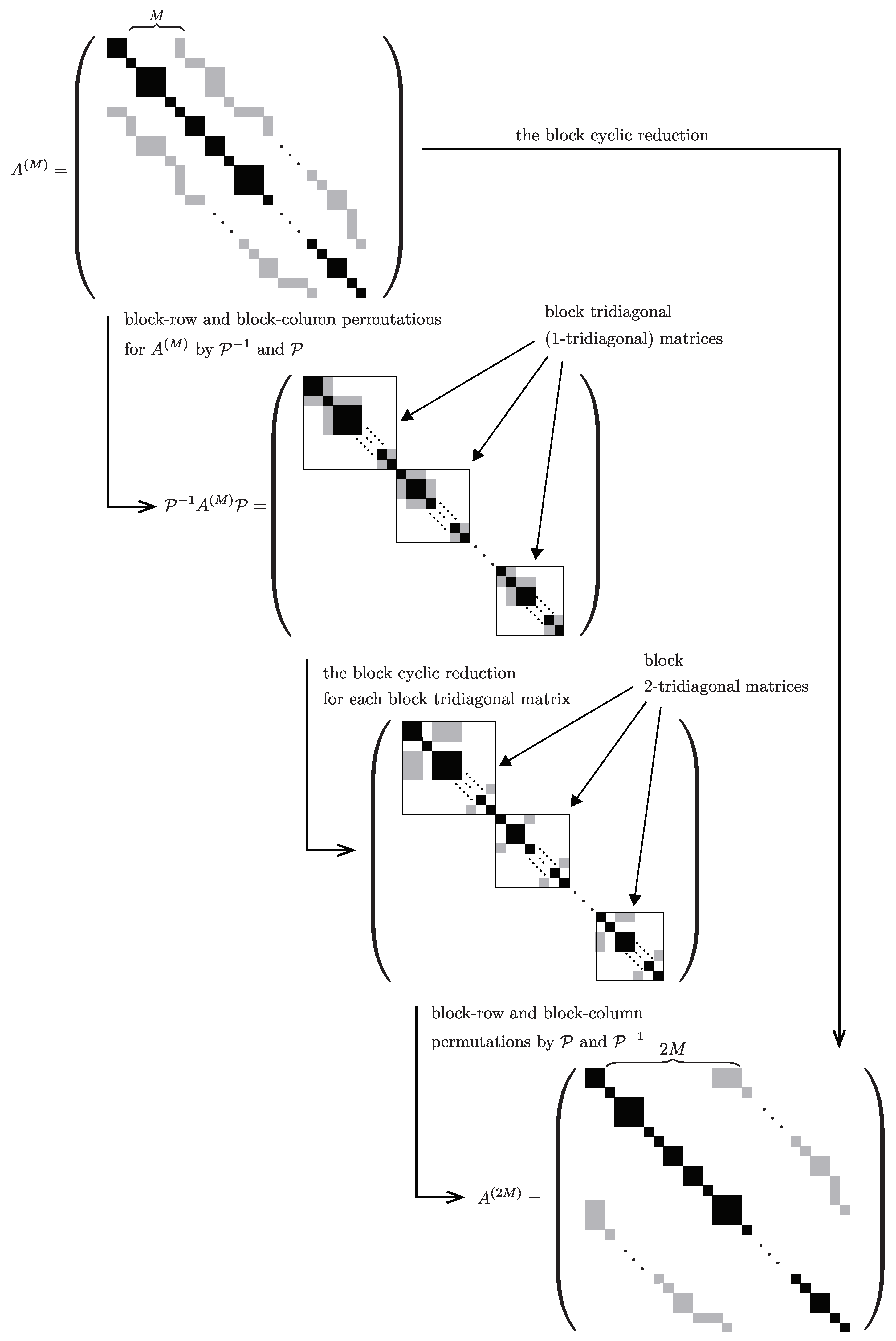
Combining (8) and (10) with (9), we obtain:

$$\begin{array}{c}\hfill {\mathcal{P}}^{-1}{A}^{\left(2M\right)}\mathcal{P}=\mathrm{diag}({\tilde{T}}_1^{\left(1\right)}{\tilde{A}}_1^{\left(1\right)},{\tilde{T}}_2^{\left(1\right)}{\tilde{A}}_2^{\left(1\right)},\cdots ,{\tilde{T}}_M^{\left(1\right)}{\tilde{A}}_M^{\left(1\right)}).\end{array}$$

(13)

This implies that the transformation from $A^{\left(M\right)}$ to $A^{\left(2M\right)}$ can also be completed using three transformations: (1) the block tridiagonalization from $A^{\left(M\right)}$ to ${\mathcal{P}}^{-1}{A}^{\left(M\right)}\mathcal{P}$; (2) the transformations from the block 1-tridiagonal matrices ${\tilde{A}}_i^{\left(1\right)}$ to the block 2-tridiagonal matrices ${\tilde{T}}_i^{\left(1\right)}{\tilde{A}}_i^{\left(1\right)}$; and (3) the block $2M$-tridiagonalization from ${\mathcal{P}}^{-1}{A}^{\left(2M\right)}\mathcal{P}$ to $A^{\left(2M\right)}$. See Figure 3 for the relationships among the block tridiagonal (1-tridiagonal), 2-tridiagonal, M-tridiagonal, and $2M$-tridiagonal matrices.

Figure 3. Coefficient matrices in the block cyclic reduction.

4. Inverses of Block 1-Tridiagonal and 2-Tridiagonal Matrices

In this section, we express the inverse of the block 1-tridiagonal matrix $A^{\left(1\right)}$ using that of the block 2-tridiagonal matrix $A^{\left(2\right)}$. This is useful for comparing the roots of the characteristic polynomials of the block 1-tridiagonal matrix $A^{\left(1\right)}$ and the block 2-tridiagonal matrix $A^{\left(2\right)}$ in the next section.

We introduce two auxiliary matrices $D:=\mathrm{diag}(D_1^{\left(1\right)},D_2^{\left(1\right)},\cdots ,D_m^{\left(1\right)})$ and $A_R^{\left(1\right)}:=R{A}^{\left(1\right)}R$, where $R:=\mathrm{diag}((-1)I_1,{(-1)}^2{I}_2,\cdots ,$${(-1)}^m{I}_m)$ involving the $N_i$-dimensional identity matrices $I_i$. Then, we derive the following lemma for an expression using D and $A_R^{\left(1\right)}$ of transformation matrix $T^{\left(1\right)}$.

Lemma 1.

The transformation matrix $T^{\left(1\right)}$ can be decomposed using D and $A_R^{\left(1\right)}$ into:

$$\begin{array}{c}\hfill T^{\left(1\right)}=A_R^{\left(1\right)}{D}^{-1}.\end{array}$$

(14)

Proof. 

It is obvious that $R{A}^{\left(1\right)}$ and $R{A}^{\left(1\right)}R$ are both block 1-tridiagonal matrices. It is easy to check that ${\left(R{A}^{\left(1\right)}\right)}_{i,j}={\left({(-1)}^j{A}^{\left(1\right)}\right)}_{i,j}$ where ${(·)}_{i,j}$ denotes the $(i,j)$ blocks of a matrix. Similarly, it turns out that ${\left(R{A}^{\left(1\right)}R\right)}_{i,j}={\left({(-1)}^{i}R{A}^{\left(1\right)}\right)}_{i,j}$. Thus, by noting that ${\left(A_R^{\left(1\right)}\right)}_{i,j}={\left({(-1)}^{i+j}{A}^{\left(1\right)}\right)}_{i,j}$, we can derive:

$$\begin{array}{c}\hfill A_R^{\left(1\right)}=\left(\begin{array}{ccc}{D}_1^{\left(1\right)}& -E_1^{\left(1\right)}& \\ -F_1^{\left(1\right)}& D_2^{\left(1\right)}& \ddots \\ & \ddots & \ddots & -E_{m-1}^{\left(1\right)}\\ & & -F_{m-1}^{\left(1\right)}& D_m^{\left(1\right)}\end{array}\right).\end{array}$$

(15)

Furthermore, it can easily be observed that $T^{\left(1\right)}D=A_R$. Noting that D is nonsingular, we obtain (14). □

Since it is obvious that $R^{-1}=R$, it holds that $A_R^{\left(1\right)}=R^{-1}{A}^{\left(1\right)}R$. This implies that the eigenvalues of $A_R^{\left(1\right)}$ coincide with those of $A^{\left(1\right)}$. Thus, $A_R^{\left(1\right)}$ is nonsingular if $A^{\left(1\right)}$ is nonsingular. From Lemma 1, it immediately follows that $det{A}^{\left(2\right)}=(det{A}_R^{\left(1\right)})(det{D}^{-1})(det{A}^{\left(1\right)})$. Therefore, the inverse of $A^{\left(2\right)}$ exists if $A^{\left(1\right)}$ is nonsingular. The following proposition gives the relationship of ${\left(A^{\left(2\right)}\right)}^{-1}$ to ${\left(A^{\left(1\right)}\right)}^{-1}$ and ${\left(A_R^{\left(1\right)}\right)}^{-1}$.

Proposition 1.

For the $(i,j)$ blocks ${\left({\left(A^{\left(1\right)}\right)}^{-1}\right)}_{i,j}$ and ${\left({\left(A^{\left(2\right)}\right)}^{-1}\right)}_{i,j}$, it holds that:

$$\begin{array}{c}\hfill {\left({\left(A^{\left(2\right)}\right)}^{-1}\right)}_{i,j}=\left\{\begin{array}{cc}{\left({\left(A^{\left(1\right)}\right)}^{-1}\right)}_{i,j}\hfill & \mathrm{if}i+j\mathrm{is}\mathrm{even},\hfill \\ O\hfill & \mathrm{if}i+j\mathrm{is}\mathrm{odd},\hfill \end{array}\right.\end{array}$$

(16)

where O denotes the zero matrix whose entries are all 0 as shown previously. Accordingly,

$$\begin{array}{c}\hfill {\left(A^{\left(2\right)}\right)}^{-1}=\frac{1}{2}({\left(A^{\left(1\right)}\right)}^{-1}+{\left(A_R^{\left(1\right)}\right)}^{-1}).\end{array}$$

(17)

Proof. 

Observing the ith block-row on both sides of the trivial identity ${\left(A^{\left(1\right)}\right)}^{-1}{A}^{\left(1\right)}=I_N$, we can obtain m matrix equations:

$$\begin{array}{c}\hfill \left\{\begin{array}{ccccccc}& & {\left({\left(A^{\left(1\right)}\right)}^{-1}\right)}_{i,1}{D}_1^{\left(1\right)}& +& {\left({\left(A^{\left(1\right)}\right)}^{-1}\right)}_{i,2}{F}_1^{\left(1\right)}& =& O,\\ {\left({\left(A^{\left(1\right)}\right)}^{-1}\right)}_{i,1}{E}_1^{\left(1\right)}& +& {\left({\left(A^{\left(1\right)}\right)}^{-1}\right)}_{i,2}{D}_2^{\left(1\right)}& +& {\left({\left(A^{\left(1\right)}\right)}^{-1}\right)}_{i,3}{F}_2^{\left(1\right)}& =& O,\\ ⋮& & ⋮& & ⋮& & ⋮\\ {\left({\left(A^{\left(1\right)}\right)}^{-1}\right)}_{i,i-1}{E}_{i-1}^{\left(1\right)}& +& {\left({\left(A^{\left(1\right)}\right)}^{-1}\right)}_{i,i}{D}_i^{\left(1\right)}& +& {\left({\left(A^{\left(1\right)}\right)}^{-1}\right)}_{i,i+1}{F}_i^{\left(1\right)}& =& I_i,\\ ⋮& & ⋮& & ⋮& & ⋮\\ {\left({\left(A^{\left(1\right)}\right)}^{-1}\right)}_{i,m-2}{E}_{m-2}^{\left(1\right)}& +& {\left({\left(A^{\left(1\right)}\right)}^{-1}\right)}_{i,m-1}{D}_{m-1}^{\left(1\right)}& +& {\left({\left(A^{\left(1\right)}\right)}^{-1}\right)}_{i,m}{F}_{m-1}^{\left(1\right)}& =& O,\\ {\left({\left(A^{\left(1\right)}\right)}^{-1}\right)}_{i,m-1}{E}_{m-1}^{\left(1\right)}& +& {\left({\left(A^{\left(1\right)}\right)}^{-1}\right)}_{i,m}{D}_m^{\left(1\right)}& & & =& O.\end{array}\right.\end{array}$$

(18)

Multiplying both sides of the 1st, 2nd, ⋯, mth equations in (18) from the right by ${\left({\left(A^{\left(1\right)}\right)}^{-1}\right)}_{1,j}$, ${\left({\left(A^{\left(1\right)}\right)}^{-1}\right)}_{2,j}$, ⋯, ${\left({\left(A^{\left(1\right)}\right)}^{-1}\right)}_{m,j}$, respectively, we can rewrite (18) as:

$$\begin{array}{c}\hfill \left\{\begin{array}{ccccccc}& & {\widehat{D}}_1^{\left(1\right)}& +& {\widehat{F}}_1^{\left(1\right)}& =& O,\\ {\widehat{E}}_1^{\left(1\right)}& +& {\widehat{D}}_2^{\left(1\right)}& +& {\widehat{F}}_2^{\left(1\right)}& =& O,\\ ⋮& & ⋮& & ⋮& & ⋮\\ {\widehat{E}}_{i-1}^{\left(1\right)}& +& {\widehat{D}}_i^{\left(1\right)}& +& {\widehat{F}}_i^{\left(1\right)}& =& {\left({\left(A^{\left(1\right)}\right)}^{-1}\right)}_{i,j},\\ ⋮& & ⋮& & ⋮& & ⋮\\ {\widehat{E}}_{m-2}^{\left(1\right)}& +& {\widehat{D}}_{m-1}^{\left(1\right)}& +& {\widehat{F}}_{m-1}^{\left(1\right)}& =& O,\\ {\widehat{E}}_{m-1}^{\left(1\right)}& +& {\widehat{D}}_m^{\left(1\right)}& & & =& O,\end{array}\right.\end{array}$$

(19)

where ${\widehat{D}}_k^{\left(1\right)}:={\left({\left(A^{\left(1\right)}\right)}^{-1}\right)}_{i,k}{D}_k^{\left(1\right)}{\left({\left(A^{\left(1\right)}\right)}^{-1}\right)}_{k,j}$, ${\widehat{E}}_k^{\left(1\right)}:={\left({\left(A^{\left(1\right)}\right)}^{-1}\right)}_{i,k}{E}_k^{\left(1\right)}{\left({\left(A^{\left(1\right)}\right)}^{-1}\right)}_{k+1,j}$ and ${\widehat{F}}_k^{\left(1\right)}:={\left({\left(A^{\left(1\right)}\right)}^{-1}\right)}_{i,k+1}{F}_k^{\left(1\right)}{\left({\left(A^{\left(1\right)}\right)}^{-1}\right)}_{k,j}$. Similarly, by focusing on the jth block column of both sides of $A^{\left(1\right)}{\left(A^{\left(1\right)}\right)}^{-1}=I_N$ and multiplying the 1st, 2nd, ⋯, mth equations from the left by ${\left({\left(A^{\left(1\right)}\right)}^{-1}\right)}_{i,1}$, ${\left({\left(A^{\left(1\right)}\right)}^{-1}\right)}_{i,2}$, ⋯, ${\left({\left(A^{\left(1\right)}\right)}^{-1}\right)}_{i,m}$, respectively, we can derive:

$$\begin{array}{c}\hfill \left\{\begin{array}{ccccccc}& & {\widehat{D}}_1^{\left(1\right)}& +& {\widehat{E}}_1^{\left(1\right)}& =& O,\\ {\widehat{F}}_1^{\left(1\right)}& +& {\widehat{D}}_2^{\left(1\right)}& +& {\widehat{E}}_2^{\left(1\right)}& =& O,\\ ⋮& & ⋮& & ⋮& & ⋮\\ {\widehat{F}}_{j-1}^{\left(1\right)}& +& {\widehat{D}}_j^{\left(1\right)}& +& {\widehat{E}}_j^{\left(1\right)}& =& {\left({\left(A^{\left(1\right)}\right)}^{-1}\right)}_{i,j},\\ ⋮& & ⋮& & ⋮& & ⋮\\ {\widehat{F}}_{m-2}^{\left(1\right)}& +& {\widehat{D}}_{m-1}^{\left(1\right)}& +& {\widehat{E}}_{m-1}^{\left(1\right)}& =& O,\\ {\widehat{F}}_{m-1}^{\left(1\right)}& +& {\widehat{D}}_m^{\left(1\right)}& & & =& O.\end{array}\right.\end{array}$$

(20)

Adding the kth equation of (19) to that of (20), multiplying this by ${(-1)}^k$, and letting $G_k^{\left(1\right)}:={\widehat{E}}_k^{\left(1\right)}+{\widehat{F}}_k^{\left(1\right)}$, we can thus obtain:

$$\begin{array}{c}\hfill {(-1)}^k(G_{k-1}^{\left(1\right)}+2{\widehat{D}}_k^{\left(1\right)}+G_k^{\left(1\right)})=\left\{\begin{array}{cc}{(-1)}^i{\left({\left(A^{\left(1\right)}\right)}^{-1}\right)}_{i,j}\hfill & \mathrm{if}k=i,\hfill \\ {(-1)}^j{\left({\left(A^{\left(1\right)}\right)}^{-1}\right)}_{i,j}\hfill & \mathrm{if}k=j,\hfill \\ O\hfill & \mathrm{otherwise},\hfill \end{array}\right.\end{array}$$

(21)

where $G_0^{\left(1\right)}:=O$ and $G_m^{\left(1\right)}:=O$. The summation for $k=1,2,\cdots ,m$ of (21) leads to:

$$\begin{array}{c}\hfill 2\sum _{k=1}^m{(-1)}^k{\widehat{D}}_k^{\left(1\right)}=[{(-1)}^i+{(-1)}^j]{\left({\left(A^{\left(1\right)}\right)}^{-1}\right)}_{i,j}.\end{array}$$

(22)

From Lemma 1, we can see that: ${\left(A^{\left(2\right)}\right)}^{-1}={\left(A_R^{\left(1\right)}{D}^{-1}{A}^{\left(1\right)}\right)}^{-1}={\left(A^{\left(1\right)}\right)}^{-1}D{\left(A_R^{\left(1\right)}\right)}^{-1}$. Since it follows from ${\left(A_R^{\left(1\right)}\right)}^{-1}={\left(R{A}^{\left(1\right)}R\right)}^{-1}=R{\left(A^{\left(1\right)}\right)}^{-1}R$ that ${\left({\left(A_R^{\left(1\right)}\right)}^{-1}\right)}_{k,j}={(-1)}^{k+j}$${\left({\left(A^{\left(1\right)}\right)}^{-1}\right)}_{k,j}$, we can obtain:

$$\begin{array}{cc}\hfill {\left({\left(A^{\left(2\right)}\right)}^{-1}\right)}_{i,j}& =\sum _{k=1}^m{(-1)}^{k+j}{\left({\left(A^{\left(1\right)}\right)}^{-1}\right)}_{i,k}{D}_k^{\left(1\right)}{\left({\left(A^{\left(1\right)}\right)}^{-1}\right)}_{k,j}\hfill \\ \hfill & =\sum _{k=1}^m{(-1)}^{k+j}{\widehat{D}}_k^{\left(1\right)}.\hfill \end{array}$$

(23)

Consequently, by combining (22) with (23), we can derive:

$$\begin{array}{c}\hfill {\left({\left(A^{\left(2\right)}\right)}^{-1}\right)}_{i,j}=\frac{1+{(-1)}^{i+j}}{2}{\left({\left(A^{\left(1\right)}\right)}^{-1}\right)}_{i,j},\end{array}$$

(24)

which implies (16). The matrix identity ${\left(A_R^{\left(1\right)}\right)}^{-1}=R{\left(A^{\left(1\right)}\right)}^{-1}R$ also gives the relationship of blocks in ${\left(A^{\left(1\right)}\right)}^{-1}$ and ${\left(A_R^{\left(1\right)}\right)}^{-1}$:

$$\begin{array}{c}\hfill {\left({\left(A_R^{\left(1\right)}\right)}^{-1}\right)}_{i,j}=\left\{\begin{array}{cc}{\left({\left(A^{\left(1\right)}\right)}^{-1}\right)}_{i,j}\hfill & \mathrm{if}i+j\mathrm{is}\mathrm{even},\hfill \\ -{\left({\left(A^{\left(1\right)}\right)}^{-1}\right)}_{i,j}\hfill & \mathrm{if}i+j\mathrm{is}\mathrm{odd}.\hfill \end{array}\right.\end{array}$$

(25)

Considering (24) and (25), we then have (17). □

Proposition 1 plays a key role in understanding the change in the roots of characteristic polynomials of coefficient matrices in linear systems after block cyclic reductions.

5. Roots of Characteristic Polynomial Sequence

In this section, we first investigate roots of characteristic polynomials of the block 2-tridiagonal matrix $A^{\left(2\right)}=T^{\left(1\right)}{A}^{\left(1\right)}$, which is transformed from the block 1-tridiagonal matrix $A^{\left(1\right)}$ in the block cyclic reduction under the assumption that $A^{\left(1\right)}$ is symmetric positive definite.

With the help of Proposition 1, we present a theorem for the roots of characteristic polynomials of $A^{\left(1\right)}$ and $A^{\left(2\right)}$.

Theorem 1.

Assume that the block tridiagonal matrix $A^{\left(1\right)}$ is symmetric positive definite. Then, for the block 2-tridiagonal matrix $A^{\left(2\right)}=T^{\left(1\right)}{A}^{\left(1\right)}$, it holds that:

$$\begin{array}{c}\hfill {\lambda }_N\left(A^{\left(1\right)}\right)\le {\lambda }_k\left(A^{\left(2\right)}\right)\le {\lambda }_1\left(A^{\left(1\right)}\right),k=1,2,\cdots ,N,\end{array}$$

(26)

where ${\lambda }_k(·)$ denotes the kth largest root of the characteristic polynomial of a matrix—namely, the kth largest eigenvalue of a matrix.

Proof. 

Let ${\mathit{u}}_1\in {\mathbb{R}}^N$ be a normalized eigenvector corresponding to ${\lambda }_1({\left(A^{\left(1\right)}\right)}^{-1}$$+{\left(A_R^{\left(1\right)}\right)}^{-1})$. Noting that ${\left(A^{\left(1\right)}\right)}^{-1}$ and ${\left(A_R^{\left(1\right)}\right)}^{-1}$ are both symmetric and considering the Rayleigh quotient [10], we can derive:

$$\begin{array}{cc}\hfill & {\mathit{u}}_1^{\top }{\left(A^{\left(1\right)}\right)}^{-1}{\mathit{u}}_1\le {\lambda }_1\left({\left(A^{\left(1\right)}\right)}^{-1}\right),\hfill \end{array}$$

(27)

$$\begin{array}{cc}\hfill & {\mathit{u}}_1^{\top }{\left(A_R^{\left(1\right)}\right)}^{-1}{\mathit{u}}_1\le {\lambda }_1\left({\left(A_R^{\left(1\right)}\right)}^{-1}\right)={\lambda }_1\left({\left(A^{\left(1\right)}\right)}^{-1}\right).\hfill \end{array}$$

(28)

This equality holds in (27) if and only if ${\mathit{u}}_1$ is the eigenvector of ${\left(A^{\left(1\right)}\right)}^{-1}$ corresponding to ${\lambda }_1\left({\left(A^{\left(1\right)}\right)}^{-1}\right)$, while the equality holds in (28) if and only if ${\mathit{u}}_1$ is also the eigenvector of ${\left(A_R^{\left(1\right)}\right)}^{-1}$ corresponding to ${\lambda }_1\left({\left(A_R^{\left(1\right)}\right)}^{-1}\right)={\lambda }_1\left({\left(A^{\left(1\right)}\right)}^{-1}\right)$. The inequalities (27) and (28) immediately lead to:

$$\begin{array}{c}\hfill {\mathit{u}}_1^{\top }({\left(A^{\left(1\right)}\right)}^{-1}+{\left(A_R^{\left(1\right)}\right)}^{-1}){\mathit{u}}_1\le 2{\lambda }_1\left({\left(A^{\left(1\right)}\right)}^{-1}\right).\end{array}$$

(29)

Using Proposition 1, we can rewrite the Rayleigh quotient ${\mathit{u}}_1^{\top }({\left(A^{\left(1\right)}\right)}^{-1}+{\left(A_R^{\left(1\right)}\right)}^{-1}){\mathit{u}}_1$ as:

$$\begin{array}{cc}\hfill {\mathit{u}}_1^{\top }({\left(A^{\left(1\right)}\right)}^{-1}+{\left(A_R^{\left(1\right)}\right)}^{-1}){\mathit{u}}_1& =2{\lambda }_1\left({\left(A^{\left(2\right)}\right)}^{-1}\right).\hfill \end{array}$$

(30)

From (29) and (30), we can see that:

$$\begin{array}{c}\hfill {\lambda }_k\left({\left(A^{\left(2\right)}\right)}^{-1}\right)\le {\lambda }_1\left({\left(A^{\left(1\right)}\right)}^{-1}\right),k=1,2,\cdots ,N.\end{array}$$

(31)

Similarly, from a comparison of the Rayleigh quotient ${\mathit{u}}_1^{\top }({\left(A^{\left(1\right)}\right)}^{-1}+{\left(A_R^{\left(1\right)}\right)}^{-1}){\mathit{u}}_1$ with the minimal eigenvalue ${\lambda }_N\left({\left(A^{\left(1\right)}\right)}^{-1}\right)$, it follows that:

$$\begin{array}{c}\hfill {\lambda }_k\left({\left(A^{\left(2\right)}\right)}^{-1}\right)\ge {\lambda }_N\left({\left(A^{\left(1\right)}\right)}^{-1}\right),k=1,2,\cdots ,N.\end{array}$$

(32)

Thus, by combining (31) with (32), we can obtain:

$$\begin{array}{c}\hfill {\lambda }_N\left({\left(A^{\left(1\right)}\right)}^{-1}\right)\le {\lambda }_k\left({\left(A^{\left(2\right)}\right)}^{-1}\right)\le {\lambda }_1\left({\left(A^{\left(1\right)}\right)}^{-1}\right),k=1,2,\cdots ,N.\end{array}$$

Since the eigenvalues of a matrix are the reciprocals of eigenvalues of its inverse matrix, we therefore have (26). □

The following theorem is a specialization of Theorem 1.

Theorem 2.

Assume that the block tridiagonal matrix $A^{\left(1\right)}$ is symmetric positive definite and that its eigenvalues are distinct from each other. Furthermore, let the non-zero blocks all be nonsingular square matrices with the same matrix size. Then, for the block 2-tridiagonal matrix $A^{\left(2\right)}=T^{\left(1\right)}{A}^{\left(1\right)}$, it holds that:

$$\begin{array}{c}\hfill {\lambda }_N\left(A^{\left(1\right)}\right)<{\lambda }_k\left(A^{\left(2\right)}\right)<{\lambda }_1\left(A^{\left(1\right)}\right),k=1,2,\cdots ,N.\end{array}$$

(33)

Proof. 

We begin by reconsidering the proof of Theorem 1. The proof of (33) is completed by proving ${\lambda }_1\left(A^{\left(1\right)}\right)>{\lambda }_1\left(A^{\left(2\right)}\right)$ and ${\lambda }_N\left(A^{\left(1\right)}\right)<{\lambda }_N\left(A^{\left(2\right)}\right)$. The equality in (31) does not hold if the equality in (29) holds. We recall here that the equality in (29) does not hold if ${\mathit{u}}_1$ is not the eigenvector of at least either ${\left(A^{\left(1\right)}\right)}^{-1}$ or ${\left(A_R^{\left(1\right)}\right)}^{-1}$ corresponding to ${\lambda }_1\left({\left(A^{\left(1\right)}\right)}^{-1}\right)={\lambda }_1\left({\left(A_R^{\left(1\right)}\right)}^{-1}\right)$. Noting that ${\lambda }_N\left(A^{\left(1\right)}\right)={\lambda }_1\left({\left(A^{\left(1\right)}\right)}^{-1}\right)$ and ${\lambda }_N\left(A^{\left(2\right)}\right)={\lambda }_1\left({\left(A^{\left(2\right)}\right)}^{-1}\right)$, we can thus see that ${\lambda }_N\left(A^{\left(1\right)}\right)<{\lambda }_N\left(A^{\left(2\right)}\right)$ if the eigenvector of $A^{\left(1\right)}$ corresponding to ${\lambda }_N\left(A^{\left(1\right)}\right)$ is not equal to that of $A_R^{\left(1\right)}$ corresponding to ${\lambda }_N\left(A_R^{\left(1\right)}\right)={\lambda }_N\left(A^{\left(1\right)}\right)$. Similarly, the inequality ${\lambda }_1\left(A^{\left(1\right)}\right)>{\lambda }_1\left(A^{\left(2\right)}\right)$ holds if the eigenvector of $A^{\left(1\right)}$ corresponding to ${\lambda }_1\left(A^{\left(1\right)}\right)$ is not equal to that of $A_R^{\left(1\right)}$ corresponding to ${\lambda }_1\left(A_R^{\left(1\right)}\right)={\lambda }_1\left(A^{\left(1\right)}\right)$.

Let us assume here that ${\mathit{v}}_1$ is the eigenvector of both $A^{\left(1\right)}$ and $A_R^{\left(1\right)}$ corresponding to ${\lambda }_1\left(A^{\left(1\right)}\right)={\lambda }_1\left(A_R^{\left(1\right)}\right)$—namely, $A^{\left(1\right)}{\mathit{v}}_1={\lambda }_1\left(A^{\left(1\right)}\right){\mathit{v}}_1$ and $A_R^{\left(1\right)}{\mathit{v}}_1={\lambda }_1\left(A^{\left(1\right)}\right){\mathit{v}}_1$. From $A^{\left(1\right)}\left(R{\mathit{v}}_1\right)=R\left(A_R^{\left(1\right)}{\mathit{v}}_1\right)$, we can then derive:

$$\begin{array}{cc}\hfill A^{\left(1\right)}\left(R{\mathit{v}}_1\right)& ={\lambda }_1\left(A^{\left(1\right)}\right)\left(R{\mathit{v}}_1\right).\hfill \end{array}$$

This implies that $R{\mathit{v}}_1$ is also the eigenvector of $A^{\left(1\right)}$ corresponding to ${\lambda }_1\left(A^{\left(1\right)}\right)$. Noting that $A^{\left(1\right)}$ does not have multiple eigenvalues, we can thus obtain ${\mathit{v}}_1=R{\mathit{v}}_1$. Let ${\mathit{v}}_1\left(i\right)$ denote the $N_i$-dimensional vector in the ith block-rows of ${\mathit{v}}_1$. Then, by observing that:

$$\begin{array}{c}\hfill \left(\begin{array}{c}{\mathit{v}}_1\left(1\right)\\ {\mathit{v}}_1\left(2\right)\\ ⋮\\ {\mathit{v}}_1\left(m\right)\end{array}\right)=\left(\begin{array}{c}-I_1\\ & I_2\\ & & \ddots \\ & & & {(-1)}^m{I}_m\end{array}\right)\left(\begin{array}{c}{\mathit{v}}_1\left(1\right)\\ {\mathit{v}}_1\left(2\right)\\ ⋮\\ {\mathit{v}}_1\left(m\right)\end{array}\right),\end{array}$$

we can specify ${\mathit{v}}_1$ as:

$$\begin{array}{cc}\hfill & {\mathit{v}}_1=\left(\begin{array}{c}\mathit{o}\\ {\mathit{v}}_1\left(2\right)\\ \mathit{o}\\ ⋮\\ {(-1)}^{m-1}{\mathit{v}}_1(m-1)\\ {(-1)}^m{\mathit{v}}_1\left(m\right)\end{array}\right),\hfill \end{array}$$

where $\mathit{o}$ denotes the zero vector whose entries are all 0. Thus, by focusing on the 1st, 3rd, ⋯, mth block rows on both sides of $A^{\left(1\right)}{\mathit{v}}_1={\lambda }_1\left(A^{\left(1\right)}\right){\mathit{v}}_1$ with odd m, we have:

$$\begin{array}{c}\hfill \left\{\begin{array}{c}{\displaystyle E_1^{\left(1\right)}{\mathit{v}}_1\left(2\right)=\mathit{o},}\hfill \\ {\displaystyle E_2^{\left(1\right)\top }{\mathit{v}}_1\left(2\right)+E_3^{\left(1\right)}{\mathit{v}}_1\left(4\right)=\mathit{o},}\hfill \\ ⋮\hfill \\ {\displaystyle E_{m-3}^{\left(1\right)\top }{\mathit{v}}_1(m-3)+E_{m-2}^{\left(1\right)}{\mathit{v}}_1(m-1)=\mathit{o},}\hfill \\ {\displaystyle E_{m-1}^{\left(1\right)\top }{\mathit{v}}_1(m-1)=\mathit{o}.}\hfill \end{array}\right.\end{array}$$

(34)

Since $E_1^{\left(1\right)}$, $E_2^{\left(1\right)}$, ⋯, $E_{m-1}^{\left(1\right)}$ are all nonsingular. (34) immediately leads to ${\mathit{v}}_1\left(2\right)=\mathit{o}$, ${\mathit{v}}_1\left(4\right)=\mathit{o}$, ⋯, ${\mathit{v}}_1(m-1)=\mathit{o}$. Namely, ${\mathit{v}}_1$ is the zero vector. This contradicts the assumption that ${\mathit{v}}_1$ is the eigenvector of both $A^{\left(1\right)}$ and $A_R^{\left(1\right)}$ corresponding to ${\lambda }_1\left(A^{\left(1\right)}\right)={\lambda }_1\left(A_R^{\left(1\right)}\right)$. The contradiction is similarly derived in the case where m is even. Therefore, we conclude that ${\lambda }_1\left(A^{\left(1\right)}\right)>{\lambda }_1\left(A^{\left(2\right)}\right)$. We also have ${\lambda }_N\left(A^{\left(1\right)}\right)<{\lambda }_N\left(A^{\left(2\right)}\right)$ along the same lines as the above proof. □

We recall here that the transformation $A^{\left(2M\right)}=T^{\left(M\right)}{A}^{\left(M\right)}$ from the block M-tridiagonal matrix $A^{\left(M\right)}$ to the block $2M$-tridiagonal matrix $A^{\left(2M\right)}$ can be regarded as a composite transformation of the transformations from the block tridiagonal matrices to the block 2-tridiagonal matrices and two similarity transformations. By combining this with Theorems 1 and 2, we can derive the following theorem concerning the roots of the characteristic polynomials of $A^{\left(M\right)}$ and $A^{\left(2M\right)}=T^{\left(M\right)}{A}^{\left(M\right)}$.

Theorem 3.

Assume that the block M-tridiagonal matrix $A^{\left(M\right)}$ is symmetric positive definite, where $M=1,2,\cdots$. Then, for the block $2M$-tridiagonal matrix $A^{\left(2M\right)}=T^{\left(M\right)}{A}^{\left(M\right)}$, it holds that:

$$\begin{array}{c}\hfill {\lambda }_N\left(A^{\left(M\right)}\right)\le {\lambda }_k\left(A^{\left(2M\right)}\right)\le {\lambda }_1\left(A^{\left(M\right)}\right),k=1,2,\cdots ,N.\end{array}$$

(35)

Furthermore, let the roots of the characteristic polynomials of $A^{\left(M\right)}$ be distinct from each other, the non-zero blocks all be nonsingular square matrices, and their matrix sizes all be the same. Then, it holds that:

$$\begin{array}{c}\hfill {\lambda }_N\left(A^{\left(M\right)}\right)<{\lambda }_k\left(A^{\left(2M\right)}\right)<{\lambda }_1\left(A^{\left(M\right)}\right),k=1,2,\cdots ,N.\end{array}$$

(36)

It is obvious that $A^{\left(2\right)}=T^{\left(1\right)}{A}^{\left(1\right)}$, $A^{\left(4\right)}=T^{\left(2\right)}{A}^{\left(2\right)}$, ⋯ are symmetric if the block tridiagonal matrix $A^{\left(1\right)}=A$ is also symmetric in the original linear system $A\mathit{x}=\mathit{b}$. From Theorem 3, we can recursively see that $A^{\left(2\right)}$, $A^{\left(4\right)}$, ⋯ are positive definite if the original coefficient matrix $A^{\left(1\right)}=A$ is also positive definite. We then conclude that:

$$\begin{array}{c}\hfill \cdots \le \frac{{\lambda }_1\left(A^{\left(2M\right)}\right)}{{\lambda }_N\left(A^{\left(2M\right)}\right)}\le \frac{{\lambda }_1\left(A^{\left(M\right)}\right)}{{\lambda }_N\left(A^{\left(M\right)}\right)}\le \cdots \le \frac{{\lambda }_1\left(A^{\left(2\right)}\right)}{{\lambda }_N\left(A^{\left(2\right)}\right)}\le \frac{{\lambda }_1\left(A^{\left(1\right)}\right)}{{\lambda }_N\left(A^{\left(1\right)}\right)},\end{array}$$

or

$$\begin{array}{c}\hfill \cdots <\frac{{\lambda }_1\left(A^{\left(2M\right)}\right)}{{\lambda }_N\left(A^{\left(2M\right)}\right)}<\frac{{\lambda }_1\left(A^{\left(M\right)}\right)}{{\lambda }_N\left(A^{\left(M\right)}\right)}<\cdots <\frac{{\lambda }_1\left(A^{\left(2\right)}\right)}{{\lambda }_N\left(A^{\left(2\right)}\right)}<\frac{{\lambda }_1\left(A^{\left(1\right)}\right)}{{\lambda }_N\left(A^{\left(1\right)}\right)},\end{array}$$

as long as the block cyclic reductions are repeated. The discussion in this section can easily be changed for the case where the original coefficient matrix $A^{\left(1\right)}=A$ is negative definite.

6. Numerical Examples

In this section, we give two examples for observing changes in coefficient matrices in the iterative block cyclic reductions for block tridiagonal linear systems $A^{\left(1\right)}\mathit{x}=\mathit{b}$ and numerically verifying Theorems 1 and 2 with respect to the roots of the characteristic polynomials of coefficient matrices. The numerical illustration was carried out on a computer; OS: Mac OS Monterey (ver. 12.0.1), CPU: 2.4 GHz Intel Core i9. For this, we employed the MATLAB software (R2021a). Computed values are given in floating-point arithmetic.

We first consider the case where $A^{\left(1\right)}$ is the 9-by-9 symmetric block tridiagonal and positive definite matrix with ${\lambda }_1\left(A^{\left(1\right)}\right)\approx 11.3465$, ${\lambda }_9\left(A^{\left(1\right)}\right)\approx 0.9931$, and ${\lambda }_1\left(A^{\left(1\right)}\right)/{\lambda }_9\left(A^{\left(1\right)}\right)\approx 11.3465/0.9931\approx 11.4253$:

$$\begin{array}{c}\hfill A^{\left(1\right)}=\left(\begin{array}{lllllllll}2& 1& 0& 0& 1& 0& 0& 0& 0\\ 1& 3& 1& 0& 0& 1& 0& 0& 0\\ 0& 1& 4& 1& 0& 0& 1& 0& 0\\ 0& 0& 1& 5& 0& 1& 0& 0& 0\\ 1& 0& 0& 0& 6& 1& 0& 1& 0\\ 0& 1& 0& 1& 1& 7& 1& 0& 1\\ 0& 0& 1& 0& 0& 1& 8& 0& 1\\ 0& 0& 0& 0& 1& 0& 0& 9& 1\\ 0& 0& 0& 0& 0& 1& 1& 1& 10\end{array}\right),\end{array}$$

(37)

where the values of ${\lambda }_1\left(A^{\left(1\right)}\right)$, ${\lambda }_9\left(A^{\left(1\right)}\right)$ and ${\lambda }_1\left(A^{\left(1\right)}\right)/{\lambda }_9\left(A^{\left(1\right)}\right)$ are computed using the MATLAB function eig and rounded to 4 digits after the decimal point. The diagonal blocks are all symmetric and their matrix sizes are distinct from one another. Since the determinants of the $(1,1)$, $(2,2)$, and $(3,3)$ blocks are, respectively, 85, 322, and 89, the diagonal blocks are all nonsingular. The non-zero subdiagonal (and superdiagonal) blocks are not square matrices, but the transposes of the $(1,2)$ and $(2,3)$ blocks coincide with those of the $(2,1)$ and $(3,2)$ blocks, respectively. After the 1st block cyclic reduction, $A^{\left(1\right)}$ is transformed to the symmetric block 2-tridiagonal matrix:

$$\begin{array}{c}\hfill A^{\left(2\right)}=\left(\begin{array}{lllllllll}\hfill 1.8292& \hfill 1.0248& \hfill -0.0031& \hfill 0.0248& \hfill 0& \hfill 0& \hfill 0& \hfill -0.1708& \hfill 0.0217\\ \hfill 1.0248& \hfill 2.8509& \hfill 1.0186& \hfill -0.1491& \hfill 0& \hfill 0& \hfill 0& \hfill 0.0248& \hfill -0.1304\\ \hfill -0.0031& \hfill 1.0186& \hfill 3.8727& \hfill 1.0186& \hfill 0& \hfill 0& \hfill 0& \hfill -0.0031& \hfill -0.1087\\ \hfill 0.0248& \hfill -0.1491& \hfill 1.0186& \hfill 4.8509& \hfill 0& \hfill 0& \hfill 0& \hfill 0.0248& \hfill -0.1304\\ \hfill 0& \hfill 0& \hfill 0& \hfill 0& \hfill 5.2759& \hfill 1.2465& \hfill -0.0476& \hfill 0& \hfill 0\\ \hfill 0& \hfill 0& \hfill 0& \hfill 0& \hfill 1.2465& \hfill 6.1930& \hfill 1.0753& \hfill 0& \hfill 0\\ \hfill 0& \hfill 0& \hfill 0& \hfill 0& \hfill -0.0476& \hfill 1.0753& \hfill 7.6048& \hfill 0& \hfill 0\\ \hfill -0.1708& \hfill 0.0248& \hfill -0.0031& \hfill 0.0248& \hfill 0& \hfill 0& \hfill 0& \hfill 8.8292& \hfill 1.0217\\ \hfill 0.0217& \hfill -0.1304& \hfill -0.1087& \hfill -0.1304& \hfill 0& \hfill 0& \hfill 0& \hfill 1.0217& \hfill 9.7609\end{array}\right),\end{array}$$

(38)

where all non-zero entries are rounded to 4 digits after the decimal point. Using the MATLAB function eig, we can see that ${\lambda }_1\left(A^{\left(2\right)}\right)\approx 10.4242$ and ${\lambda }_9\left(A^{\left(2\right)}\right)\approx 1.0440$. Thus, ${\lambda }_1\left(A^{\left(2\right)}\right)/{\lambda }_9\left(A^{\left(2\right)}\right)\approx 9.9849<{\lambda }_1\left(A^{\left(1\right)}\right)/{\lambda }_9\left(A^{\left(1\right)}\right)$. It is also easy to check that the diagonal blocks of $A^{\left(2\right)}$ are all nonsingular. This implies that a block cyclic reduction can again be applied to the linear system with the coefficient matrix $A^{\left(2\right)}$. The 2nd block cyclic reduction then simplifies $A^{\left(2\right)}$ as the block diagonal matrix:

$$\begin{array}{c}\hfill \mathcal{A}=\left(\begin{array}{lllllllll}\hfill 1.8257& \hfill 1.0259& \hfill -0.0027& \hfill 0.0259& \hfill 0& \hfill 0& \hfill 0& \hfill 0& \hfill 0\\ \hfill 1.0259& \hfill 2.8490& \hfill 1.0171& \hfill -0.1510& \hfill 0& \hfill 0& \hfill 0& \hfill 0& \hfill 0\\ \hfill -0.0027& \hfill 1.0171& \hfill 3.8715& \hfill 1.0171& \hfill 0& \hfill 0& \hfill 0& \hfill 0& \hfill 0\\ \hfill 0.0259& \hfill -0.1510& \hfill 1.0171& \hfill 4.8490& \hfill 0& \hfill 0& \hfill 0& \hfill 0& \hfill 0\\ \hfill 0& \hfill 0& \hfill 0& \hfill 0& \hfill 5.2759& \hfill 1.2465& \hfill -0.0476& \hfill 0& \hfill 0\\ \hfill 0& \hfill 0& \hfill 0& \hfill 0& \hfill 1.2465& \hfill 6.1930& \hfill 1.0753& \hfill 0& \hfill 0\\ \hfill 0& \hfill 0& \hfill 0& \hfill 0& \hfill -0.0476& \hfill 1.0753& \hfill 7.6048& \hfill 0& \hfill 0\\ \hfill 0& \hfill 0& \hfill 0& \hfill 0& \hfill 0& \hfill 0& \hfill 0& \hfill 8.8052& \hfill 1.0321\\ \hfill 0& \hfill 0& \hfill 0& \hfill 0& \hfill 0& \hfill 0& \hfill 0& \hfill 1.0321& \hfill 9.7475\end{array}\right).\end{array}$$

(39)

The MATLAB function eig immediately returns ${\lambda }_1\left(\mathcal{A}\right)\approx 10.4109$ and ${\lambda }_9\left(\mathcal{A}\right)\approx 1.0445$. Therefore, ${\lambda }_1\left(\mathcal{A}\right)/{\lambda }_9\left(\mathcal{A}\right)\approx 9.9674<{\lambda }_1\left(A^{\left(2\right)}\right)/{\lambda }_9\left(A^{\left(2\right)}\right)$.

Next, we deal with the case where $A^{\left(1\right)}$ is the 9-by-9 symmetric block tridiagonal and negative definite matrix with ${\lambda }_1\left(A^{\left(1\right)}\right)=-1.172$, ${\lambda }_9\left(A^{\left(1\right)}\right)=-6.828$ and ${\lambda }_1\left(A^{\left(1\right)}\right)/{\lambda }_9\left(A^{\left(1\right)}\right)\approx 6.828/1.172\approx 5.826$,

$$\begin{array}{c}\hfill A^{\left(1\right)}=\left(\begin{array}{lllllllll}\hfill -4& \hfill 1& \hfill 0& \hfill 1& \hfill 0& \hfill 0& \hfill 0& \hfill 0& \hfill 0\\ \hfill 1& \hfill -4& \hfill 1& \hfill 0& \hfill 1& \hfill 0& \hfill 0& \hfill 0& \hfill 0\\ \hfill 0& \hfill 1& \hfill -4& \hfill 0& \hfill 0& \hfill 1& \hfill 0& \hfill 0& \hfill 0\\ \hfill 1& \hfill 0& \hfill 0& \hfill -4& \hfill 1& \hfill 0& \hfill 1& \hfill 0& \hfill 0\\ \hfill 0& \hfill 1& \hfill 0& \hfill 1& \hfill -4& \hfill 1& \hfill 0& \hfill 1& \hfill 0\\ \hfill 0& \hfill 0& \hfill 1& \hfill 0& \hfill 1& \hfill -4& \hfill 0& \hfill 0& \hfill 1\\ \hfill 0& \hfill 0& \hfill 0& \hfill 1& \hfill 0& \hfill 0& \hfill -4& \hfill 1& \hfill 0\\ \hfill 0& \hfill 0& \hfill 0& \hfill 0& \hfill 1& \hfill 0& \hfill 1& \hfill -4& \hfill 1\\ \hfill 0& \hfill 0& \hfill 0& \hfill 0& \hfill 0& \hfill 1& \hfill 0& \hfill 1& \hfill -4\end{array}\right).\end{array}$$

(40)

This is an example matrix appearing in the discretization of Poisson’s equation [11]. It is different from the 1st example matrix in that all the blocks have the same matrix size. It is obvious that the non-zero blocks are all 3-by-3 nonsingular. A block cyclic reduction then transforms $A^{\left(1\right)}$ into the symmetric block 2-tridiagonal matrix:

$$\begin{array}{c}\hfill A^{\left(2\right)}=\left(\begin{array}{lllllllll}\hfill -3.7321& \hfill 1.0714& \hfill 0.0179& \hfill 0& \hfill 0& \hfill 0& \hfill 0.2679& \hfill 0.0714& \hfill 0.0179\\ \hfill 1.0714& \hfill -3.7143& \hfill 1.0714& \hfill 0& \hfill 0& \hfill 0& \hfill 0.0714& \hfill 0.2857& \hfill 0.0714\\ \hfill 0.0179& \hfill 1.0714& \hfill -3.7321& \hfill 0& \hfill 0& \hfill 0& \hfill 0.0179& \hfill 0.0714& \hfill 0.2679\\ \hfill 0& \hfill 0& \hfill 0& \hfill -3.4643& \hfill 1.1429& \hfill 0.0357& \hfill 0& \hfill 0& \hfill 0\\ \hfill 0& \hfill 0& \hfill 0& \hfill 1.1429& \hfill -3.4286& \hfill 1.1429& \hfill 0& \hfill 0& \hfill 0\\ \hfill 0& \hfill 0& \hfill 0& \hfill 0.0357& \hfill 1.1429& \hfill -3.4643& \hfill 0& \hfill 0& \hfill 0\\ \hfill 0.2679& \hfill 0.0714& \hfill 0.0179& \hfill 0& \hfill 0& \hfill 0& \hfill -3.7321& \hfill 1.0714& \hfill 0.0179\\ \hfill 0.0714& \hfill 0.2857& \hfill 0.0714& \hfill 0& \hfill 0& \hfill 0& \hfill 1.0714& \hfill -3.7143& \hfill 1.0714\\ \hfill 0.0179& \hfill 0.0714& \hfill 0.2679& \hfill 0& \hfill 0& \hfill 0& \hfill 0.0179& \hfill 1.0714& \hfill -3.7321\end{array}\right),\end{array}$$

(41)

where ${\lambda }_1\left(A^{\left(2\right)}\right)=-1.8123$, ${\lambda }_9\left(A^{\left(2\right)}\right)=-5.4142$, and ${\lambda }_1\left(A^{\left(2\right)}\right)/{\lambda }_9\left(A^{\left(2\right)}\right)\approx 2.9875$. Since the non-zero blocks in $A^{\left(2\right)}$ are all nonsingular, we can simplify $A^{\left(2\right)}$ as the block diagonal matrix:

$$\begin{array}{c}\hfill \mathcal{A}=\left(\begin{array}{lllllllll}\hfill -3.7052& \hfill 1.0932& \hfill 0.0282& \hfill 0& \hfill 0& \hfill 0& \hfill 0& \hfill 0& \hfill 0\\ \hfill 1.0932& \hfill -3.6770& \hfill 1.0932& \hfill 0& \hfill 0& \hfill 0& \hfill 0& \hfill 0& \hfill 0\\ \hfill 0.0282& \hfill 1.0932& \hfill -3.7052& \hfill 0& \hfill 0& \hfill 0& \hfill 0& \hfill 0& \hfill 0\\ \hfill 0& \hfill 0& \hfill 0& \hfill -3.4643& \hfill 1.1429& \hfill 0.0357& \hfill 0& \hfill 0& \hfill 0\\ \hfill 0& \hfill 0& \hfill 0& \hfill 1.1429& \hfill -3.4286& \hfill 1.1429& \hfill 0& \hfill 0& \hfill 0\\ \hfill 0& \hfill 0& \hfill 0& \hfill 0.0357& \hfill 1.1429& \hfill -3.4643& \hfill 0& \hfill 0& \hfill 0\\ \hfill 0& \hfill 0& \hfill 0& \hfill 0& \hfill 0& \hfill 0& \hfill -3.7052& \hfill 1.0932& \hfill 0.0282\\ \hfill 0& \hfill 0& \hfill 0& \hfill 0& \hfill 0& \hfill 0& \hfill 1.0932& \hfill -3.6770& \hfill 1.0932\\ \hfill 0& \hfill 0& \hfill 0& \hfill 0& \hfill 0& \hfill 0& \hfill 0.0282& \hfill 1.0932& \hfill -3.7052\end{array}\right),\end{array}$$

(42)

with ${\lambda }_1\left(\mathcal{A}\right)=-1.8123$, ${\lambda }_9\left(\mathcal{A}\right)=-5.2230$, and ${\lambda }_1\left(\mathcal{A}\right)/{\lambda }_9\left(\mathcal{A}\right)=2.8820$. Thus, it can numerically be observed that: ${\lambda }_1\left(A^{\left(1\right)}\right)/{\lambda }_9\left(A^{\left(1\right)}\right)>{\lambda }_1\left(A^{\left(2\right)}\right)/{\lambda }_9\left(A^{\left(2\right)}\right)>{\lambda }_1\left(\mathcal{A}\right)/{\lambda }_9\left(\mathcal{A}\right)$.

7. Concluding Remarks

This paper focused on coefficient matrices in linear systems obtained from block iterative cyclic reductions. We showed that block M-tridiagonal coefficient matrices can be transformed to block tridiagonal matrices without changing the eigenvalues. We interpreted transformations from block M-tridiagonal matrices to block $2M$-tridiagonal matrices as composite transformations of the block tridiagonalizations, with their inverses and transformations from block tridiagonal matrices to block 2-tridiagonal matrices appearing in the first step of the block cyclic reduction method. We then used this interpretation to consider the other steps of the block cyclic reduction method. We found a relationship between the inverses of block tridiagonal matrices and block 2-tridiagonal matrices in the first step, which helped us to clarify the main results of this paper—i.e., the first step narrows the distribution of roots of characteristic polynomials associated with coefficient matrices, and the other steps also do this if the original coefficient matrices are symmetric positive or negative definite. This property suggests that each block cyclic reduction does not make it difficult to solve a linear system with a symmetric positive or negative definite block tridiagonal matrix, which will be useful for dividing a large-scale linear system into several small-scale ones.

A remarkable point of our approach is, as a result, useful regardless of whether coefficient matrices are tridiagonal or block tridiagonal. However, the coefficient matrices are currently limited to be symmetric positive or negative definite. For example, in the nonsymmetric Toeplitz case [12], our approach cannot grasp root distribution of the characteristic polynomial. Future work thus involves developing our approach so that root distribution can be examined in the cases of various coefficient matrices.