Abstract
The paper presents a mathematical modeling approach to determine the permanent regime temperature of an electric contact found in the supply system of the railway electric traction. Mathematical modeling is a basic procedure in the preliminary determination of parameters of interest in various fields of scientific analysis. The numerical modeling method used for determining the electric contact temperature represents the base for developing a finite-element thermal model. The simulation of the electric contact was verified by an experimental infrared investigation of an electric contact realized on a realistic laboratory setup. The results interpretation reveals a good synchronization between the calculated, simulated and measured temperatures.
1. Introduction
In order to perform the diagnosis of the technical condition of an electrical equipment, it is also necessary to know its thermal stresses. The degree of thermal stress has a direct influence on technical and economic aspects and implicitly on the maintenance of electrical equipment. Excessive heating (hyperthermia) endangers the proper functioning of the equipment and shortens its service life (operation), and too low heating (hypothermia) leads to an oversized construction, economically unreasonable [1,2,3].
The supervision of temperature in the case of equipment in operation is difficult to achieve. Currently, the supervision of the temperature of the equipment within the power system (equipment in substations and substations) is mostly carried out occasionally. Surveillance installations from the simplest to the most complicated are based on the detection of infrared radiation emitted by warmer bodies [4,5]. By directly viewing the supervised equipment, the warmest points on the current path are detected. In this way, the places where it is necessary to be intervened to restore the contact links are determinate. In this case, it becomes necessary to move the monitored equipment in to the area where these thermal imaging can be properly taken, which sometimes is difficult to achieve [6].
In the electrical equipment under operation, heat is permanently developed, due to the transformation of a part of the electromagnetic energy into thermal energy, at the level of different constructive elements [7]. In normal operating mode, the temperatures of the different constructive parts of it increase over time until the values corresponding to the stationary thermal regime are reached. At this point all the heat released in the equipment is given to the environment as a result of the heat released in the equipment [8,9]. In the case of the heating regimes produced by the short circuit currents, the thermal process can be considered adiabatic, so the entire thermal energy released is leading to increasing the electrical equipment constructive elements temperatures towards high values [10].
In order to guarantee the electrical equipment proper operation in terms of temperature, the standards impose (depending on the materials used and the operating conditions) certain maximum permissible limits, both for the stationary temperatures and for the short-term regime ones [11].
The use of mathematical modeling to determine or anticipate certain parameters that denote the technical condition of the devices is common in the industry. In Table 1, some of the applications based on mathematical modeling are centralized.

Table 1.
Mathematical parameters determination used for a specific application.
In [22], the authors presented a calculation mathematical model for electromotive force, respectively magnetomotive force with the aim of presenting a novel skew angle for reducing the 17th harmonic, which had the biggest magnitude among the harmonics according to their research. Moreover, a prediction model of hot spot temperature for split-windings electric traction transformer was also modeling by mathematical determination and applied in simulation according to the authors of [23]. As stated in literature, mathematical modulation helps also in determination of thermal and electrical performance in high-voltage power modules as in [24] scientific research of nonmetallic additively manufactured impingement coolers.
Transient thermal effects are presenting a high point of interest in domain of railway traction motors, as presented in [25] the authors propose a mathematical model for heat transfer from the end winding to the air, which did simulate it in finite element software and then did validate it by experimental setup and temperature measurements performed in laboratory.
In this article, it is proposed the modeling by mathematical calculation, the simulation with the use of FEM (finite element analysis) software, as well as the validation by infrared monitoring of the electrical contacts temperature evolution. The electrical contact is part of the return circuit of railway electric traction power supply system. For this, the temperature of the electrical contacts belonging to an electrical equipment (impedance bond) are modeled by mathematical calculation, and then is a study performed by COMSOL Multiphysics version 5.6 software environment for the electric contacts heating transitional regimes, in 4 connection configurations. By performing infrared monitoring during laboratory tests, the validation of calculations and simulation was performed.
The main purpose of the article is to highlight the importance of mathematical modeling when it is necessary to anticipate temperature evolution in the constructive elements passed thru by electric currents. The main difference compared to other studies [26,27,28,29] is represented by the approach adopted in order to equivalate mathematical modeling with FEM simulation. The article’s aim is to provide mathematical modeling of temperature evolution within electrical contacts and to transpose this into a FEM analysis model which can be further used in estimating temperature for different values of currents passed thru. As the state of the art [30,31] in regard to mathematics applied in industry temperature anticipation, and also validated by means of infrared investigation [31], the present article provides particular mathematical equations applied in electrical installation in order to calculate, simulate the temperature evolution for a specific electrical application from the return circuit of railway electric traction. Validation experiment conducted by infrared investigations refers to a portion of the power supply system return circuit of electric traction which uses a single-phase current with a frequency of 50 Hz and a voltage of 25 kV, specific for Romanian railway electric traction. This portion of the power supply system return circuit focuses on the electrical contact between impedance bond and connection conductors to the railway rails.
2. Mathematic Determination θ of Electrical Contact Temperature
The temperature of an electrical equipment is determined by the ambient temperature θa (of the place where it is located), to which is added the temperature increase due to the heating of the equipment by electrocaloric effect ϑ (named overtemperature):
The main sources of heat in electrical equipment are especially conductors traveled by electric current and iron cores crossed by the magnetic flux variable over time. In the case of switching equipment, we will consider that the development of heat occurs in the current pathways by electrocaloric effect.
Transient temperature of electrical equipment occurs due to the change in their operating states. Among the most characteristic transient requests of the electrical equipment, related to their working regime, we mention: the process of heating the equipment during the supply from the network, until the stationary thermal regime is reached; the process of cooling after disconnection from the network; the process of heating at short load; the process of heating at periodic intermittent regime; the process of heating at short circuit regime [32].
Transient thermal stress may also occur due to internal heat sources, related to the normal operation of the equipment or in case of damage (the occurrence of the electric arc between the contacts or in the case of a damage through the contouring arch, hot gases and vapors of molten metal etc.). In all the mentioned cases, the metallic or dielectric construction parts of the equipment will be highly thermally stressed, diminishing its reliability [32].
2.1. General Equation of Current Paths Temperature Evolution
General equation of current paths temperature evolution, has the expression [33]:
where p (x, t) represents the specific power losses in the conductor, γ—the density of the material; c—the specific heat, λ—the thermal conductivity of the current path material, αt(x, t)—represents the overall thermal transmissivity; lpx—the perimeter of the cross-section sx of the current path.
For a homogeneous portion of a current path, having the section s and the perimeter of lp constants along the entire length, the Equation (2) becomes of the form:
By making the change of variable (1), the Equation (3) becomes:
where ϑ (x, t) represents the overtemperature of the current path.
Solving this equation, taking into account all the factors that enter the thermal phenomena, involves great difficulties of calculation and in certain engineering applications, and this effort has no justification.
Furthermore, long term temperature evolution calculation is carried out on the basis of the following simplifying hypotheses: the conductive path is homogeneous, the global thermal transmissivity and the specific heat are considered invariable with the temperature, the temperature variation along the conductor is null, and the ambient temperature has a constant value. In these cases, the Equation (4) according to [34,35,36,37], become:
And will have a final form as:
where ρ0—represents the resistivity of the conducting material at 0 °C; γ—the density of the conductive material at 0 °C; —the coefficient of variation of the resistivity with the temperature; J—the current density; c—the specific heat; —the global thermal transmissivity; ℓp—the length of the perimeter corresponding to the cross-section s; —overtemperature of the conductive path.
If noted:
The differential Equation (6) is written as:
In the hypothesis of the critical value of the current density, given by the relation:
for which the denominator of the expressions (7) is cancelled, Equation (8) becomes:
and admits the solution:
In the hypothesis J ≠ Jcr, the differential Equation (5) has as its solution the expression:
where and T, given by relation (7), represent the overtemperature of permanent regime, respectively the thermal time constant of the conductor.
It is known that if a system can be described mathematically, then it is possible to find a system of a different nature who’s its evolution is expressed by the same equation [8,32,38,39,40,41]. Thus, there is an opportunity to study thermal processes with a system of an electrical nature. At the same time, a simple and quite general method of analyzing the thermal field in an electrical equipment in a stationary thermal state can be analyzed in [42,43,44].
2.2. Temperature Evolution Determination of Conductive Paths with Different Cross-Sections
The stationary heating regime of the conductive paths is characterized by temperature invariable values in time. For the analysis of this regime, the general equations of thermal conduction, respectively of the temperature evolution of the conductive paths [44,45] are used. From the calculation point of view, the permanent regime can be approached in simplifying hypotheses, when the existence of an equalizing axial thermal flux is not taken into account or, in an understanding closer to reality, when the permanent regime is studied in the presence of this thermal flux.
In permanent mode, the axial thermal flow of heat transmission by conduction along a conductive path having a constant surface cross-section can be neglected, in general, if the length of the conductor is large enough or if it is provided at the ends with very good quality thermal insulation. Under these conditions, at permanent regime, the temperature along the conductive path is considered constant. From Equation (5) we obtain:
Equation (13) emphasizes the fact that, in permanent mode, the heat released by electrocaloric effect in a conductor, without axial thermal flux, is fully transmitted to the environment. In order to determine the specific losses p, in alternating current it is necessary to consider the additional losses, which occur due to the pellicle and proximity effects [32,46]. In general, the specific losses in the volume of conductors can be calculated with the relation:
where the notations have the following meanings: kp—the coefficient of additional losses (kp = 1 in dc, kp > 1 in ac); —the resistivity at 0 °C; αR—the thermal coefficient of the resistivity; I—the effective value of the intensity of the conduction current; s—the surface of the cross-section of the conductive path. Taking into account Equation (14), the thermal balance [47] equation takes the form:
If a conductive path traveled by the load current I = Is reaches, in permanent heating regime, the temperature of constant value θ = θp, then from (15) we obtain:
In the hypothesis θp = θad, with θad being the permissible temperature corresponding to the long-term thermal stress, from (15) results the expression of the permissible current intensity [32,48]:
The Equation (16) also allows the calculation of the cross-section of the conductive path surface dimensions, for specified values of the load current Is, respectively of the permanent regime temperature, which is θp < θad [32]. Thus, for an insulated conductive path with circular cross-section, Figure 1, with a diameter noted dc, it can be made the replacement with the following equivalent formulas:
that from (17) the following is obtained:
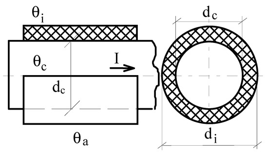
Figure 1.
Insulated current path with circular cross-section.
For the determination of temperature θc, from the conducting volume of an isolated current path (Figure 1), the following expression is used:
where q—is the density of the thermal flow; λ—the thermal conductivity of the insulating material.
Because of per unit of the conductive path length, the density of the radial heat transmission heat flow of is given by the relation:
P being the radial thermal flux, the Equation (21) becomes of the form:
which, by integrating of the insulating layer thickness, leads to the solution:
where θc, θi are the temperatures in the volume of the conductor, respectively of the insulation, and dc, di- the diameters of the current path (Figure 1).
On the other hand, it can be written:
θa, αt being the ambient temperature, respectively the thermal transmissivity to the outer surface of the current path. Taking into account the relations (23), (24), it is obtained:
Taking into account the relations for the thermal flow P, considered per unit of the current path length, the relationship is established:
p—being the specific losses by electrocaloric effect in the conductor, given by relation (14); and from the relations (14), (24), (25), for the permanent regime temperature in the conductor’s volume, the expression is obtained:
where it was noted:
Rθ—representing the resulting thermal resistance, considered in the radial direction of heat transmission. The relations from (25), (26) allow the calculation of the permanent regime temperature corresponding to an isolated current path, crossed by a charge current, as well as the determination of the permissible current intensity; the same relationships can be used for the sizing of the current path, when the current load intensity and the permanent regime temperature are known.
In the case of conductors with rectangular section, Figure 2, imposing a value for the sides ratio, a/b = n, it results:
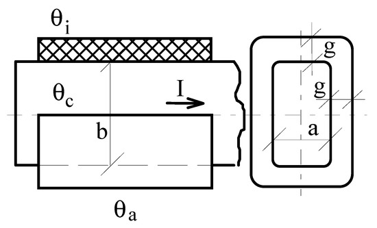
Figure 2.
Insulated current path with rectangular cross-section.
For the current path rectangular cross-section, the calculation of the permanent regime temperature is performed in the simplifying hypotheses according to which it is constant in the volume of the conductor, and on the current path outer surface being considered constants the density of the heat exchange thermal flow, respectively the global thermal transmissivity. On either of the two perpendicular directions of heat transmission by conduction in the insulating layer, the Equation (20) is written as:
and by integrating on the insulation thickness g, it is obtained:
where it is results:
θc, θi—being the temperatures of the conductor, respectively of the insulation; and λ—the thermal conductivity of the insulation. Newton’s relationship, considered on the outer surface of the insulation, is in the form of:
where θa is the environment temperature. On the basis of Equations (28) and (29) it is obtained:
If P represents the thermal flux per unit over the conductor length, for the density of heat flow the relationship can be written as:
and taking into account (14), for the heat flow density shall be finally obtained the following equation:
The relations (33), (35) lead to the permanent regime temperature θc, defined by the expression:
where it was noted:
The Equations (36) and (37) allow similar determinations to those in the case of circular cross-section current path.
The temperature evolution of the conductive paths, uninsulated or insulated, from the return circuit of the railway electric traction supply system (with circular or rectangular section) can be determined by applying the previous models.
2.3. Electrical Contacts Temperature Evolution Determination
2.3.1. Contact Resistance General Aspects
Electrical contacts are constructive elements of the current paths consisting of metal parts by touching which the electrical conduction is obtained.
Touching the contact parts is performed under the action of a force Fc, named contact force, usually produced by means of mechanical devices (pre-tensioned springs).
The presence of an electrical contact on a current path always introduces an additional passing resistance, called contact resistance, Rc [40].
The existence of contact resistance is explained on account of two processes that are highlighted at the level of contact: the restriction of the current lines and the covering of the contact surfaces with disturbing films [40].
It is thus considered that the contact resistance has two components, the stricture resistance, Rs, respectively the pellicular resistance, Rp [40].
Regardless of the contact surfaces roughness, their touch can only take place in a finite number of points, Figure 3a; under these conditions, the actual contact surface, Ac, always results in much smaller than the apparent contact surface, dependent on the geometric dimensions of the parts [40].
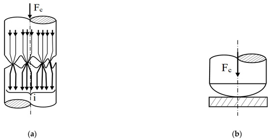
Figure 3.
Electrical contacts: (a) roughness of the contact surface; (b) finger point contact.
The actual contact surface, Ac [m2], can be calculated with the relation given by Holm:
where Fc [N]—is the contact force; H [N/m2]—hardness of the contact material; n—the number of contact microsurfaces; a [m]—the radius of a microsurface considered circular, ξ < 1—the coefficient of hardness H correction, having lower values in the case of contact peaks than those determined macroscopically [40].
For finger point contacts, Figure 3b, the actual contact area is calculated with the relation:
The hardness H of the contacts is of the same nature as the Brinell hardness, but of different values [47], in the case of electrical contacts it is generally lower [48]; for these reasons, the hardness H can be successfully replaced in the calculations by the contact material crushing resistance, σp [N/m2] [40].
From the above it is concluded that the stricture resistance is a consequence of the discontinuity of the transverse surface of the current path in the area of the electrical contact.
The stricture resistance, Rs [Ω], for a finger point contact is determined on the infinite conductivity sphere model theory basis, respectively of the elliptical contact microsurface model [4,49], being given by the relations:
where ρ [Ωm]—is the resistivity of the contact material; a [m]—the radius of the contact microsurface.
According to the sphere of infinite conductivity model, it is considered that between two metal parts 1, 2, (Figure 4a), having the resistivity ρ ≠ 0, the elementary electrical contact is made by means of a sphere, having the radius a and the resistivity is null. In these conditions, in the contact place area, the current lines are radial, and the equipotential surfaces are spheres, concentric with the contact sphere.
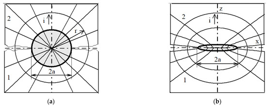
Figure 4.
The stricture resistance approximation: (a) the infinite conductivity sphere model; (b) the elliptical contact microsurface model.
In the case of the elliptical contact microsurface model, the contact surface between the metal parts 1, 2 (Figure 4b), is considered to be made after an ellipse of semi axes marked with a, b; thus, the current lines are oriented by the geodesic curves at the surfaces of the hyperboloids with a single canvas, which have as curves the necklace ellipses confocal with the contact ellipse, and the equipotential surfaces being ellipsoids, also confocal with this ellipse.
Regardless of the model used, for the calculation of the stricture resistance, a process based on the duality existing between the relations that characterize the electrostatic field in vacuum and the stationary electric field of the continuous currents, used in a conductive environment.
The pellicular resistance, Rp, is highlighted as a result of the disturbing films formation over the contact surfaces, which have semiconductor properties. The chemical composition and thickness of the disturbing film depend on the nature of the contact material; the operating temperatures; as well as the chemical composition of the environment in which the electrical contacts operate.
The pellicular resistance, Rp [Ω], can be calculated with a relationship of the form:
where Rpo [Ωm2]—is the specific superficial resistance; and Ac [m2]—the actual contact surface.
In the ordinary design practice, the calculation of electrical contacts is performed taking into account only the stricture resistance; corrections shall be introduced also the pellicular resistance, will be made by means of the following equation:
Taking into account (39)–(41), for a contact with n touch points, in the calculation of which the spherical model of the contact microsurface is adopted, the Equation (42) becomes of the form:
In the case of finger point contact, the radius of the circular contact microsurface is calculated with the relation (39), from which results:
and substituting (38) in (40), it will be obtained:
The relationship (44) highlights the fact that an electrical contact can be assimilated to a portion of the current path, having the electrical resistance dependent on the values of the pressing force Fc [40].
For a contact with n points of touch, by excluding the parameter a from the Equations (38) and (43), it is obtained:
For the contact resistance determination in the case of contacts made by metallic coatings, the resistivity of the base material and the hardness of the material used for coating are considered according to [4].
In the calculation of electrical contacts, the relationship (43) is usually considered in the restricted form as:
the values of the parameters c, m, e being determined by experimental means.
In Table 2 there are given the values of the parameters c and e, according to [4,50], for other parameters is adopted m = 0.6, Rpo = 10−12 [Ω m2], ξ = 0.45, according to [50].
Table 2.
Approximation function coefficients which are associated with the most common materials used for electrical contacts.
2.3.2. Modelling Electrical Contacts Permanent Heating Regime
Any electrical contact closed and passed by current is the seat of electrocaloric transformations, produced by the Joule–Lenz effect.
It is considered a fixed contact, passed by the current of mi intensity, where m is the number of current tubes that run through the contact surface. In Figure 5 are represented such tubes, which approximate each (in the plane of the contact surface) the area sc. Current passage is characterized by the equipotential and, at the same time, isothermal sx surface; on the surface of the sc is recorded (in permanent heating regime) the temperature θc. The voltage drop on the contact piece is measured along the current tube, in relation to the contact surface voltage, which is considered null, uc (0) = 0.
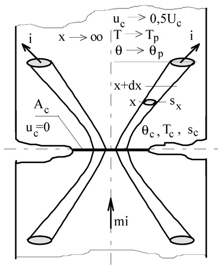
Figure 5.
Electrical contact permanent heating regime.
If it is considered that there is no caloric exchange between the current tubes, the thermal flows of heat transmission by conduction being directed only along them, for the thermal flow Px, corresponding to an isothermal sx surface, according to Fourier’s law, the expression results:
The Px thermal flow can be written successively in the forms of:
Relations (48), (49) lead to the equation:
In the hypothesis that the temperature of permanent regime θc, on the contact surface, slightly exceeds the temperature θp, recorded at a point sufficiently far from the contact area of the current path, θc − θp = 5 ÷ 10 °C, the Equation (50) is, and also is considering the multiplication between λρ to be its constant average value, (λρ)med. Through integration, the relation of Kohlrausch results, written in the form of:
or rewrite it as:
For a point of the current path, sufficiently far from the contact, characterized by the permanent regime temperature θp and the voltage drop over contact surface is half of the voltage drop over entire contact, uc = 0.5 Uc, the relation (52) becomes of the form:
where Uc—being the voltage drop on the entire contact; θ c-temperature of the contact surface permanent regime.
If temperature θc has values close to the melting point of the contact metal, the equation (50) is integrated into the hypothesis of Wiedemann-Franz-Lorenz law:
where λ, ρ—represents the thermal conductivity, respectively the resistivity of the contact parts metal; T—their absolute temperature, and L = 2.4 × 10⁻⁸ lorenz number for metals. Because dθ = dT, from (50) it is obtained:
or rewrite as:
where Tc—being the contact surface temperature.
For an equipotential (isothermal) surface, located at a sufficiently far distance from the contact surface (x → ∞, as in Figure 5), and also considering T = TP, uc = 0.5 Uc, the relation (56) becomes of the form:
The relation (57) allows the calculation of the permanent regime temperature, Tc, of the contact surface, when the values of the voltage drop on the contact, UC, (which can be easily measured) and the permanent regime temperature TP corresponding to a point of the current path (sufficiently distant from the contact surface) are known.
The permanent heating regime is verified by the relation:
where Tc—is the contact surface temperature, calculated with relation (57); and —the maximum admissible temperature corresponding to the long-term thermal stress.
For the most common types of contacts, in Table 3 are listed their values.
Table 3.
Maximum admissible temperature corresponding to electrical contact type.
For the determination of the apparent contact surfaces, in the calculations are used values of the maximum admissible current density, Jad, which is usually determined by experimental means.
Thus, for copper contacts, it can be considered the followings reference values [4,50]:
3. Experimental Results and Discussion
3.1. Case study Premises-Experimental Setup
In order to implement and validate the mathematical models presented in the previous section, an experiment was carried out in the laboratory to analyze the temperature evolution of an electrical contacts found in the connection configuration of an impedance bond, which is found in the return circuit of the electric traction electricity supply system.
In Figure 6 is presented an image of a jot coil connected by connecting ropes to two running rails and the contact areas that appear between them.
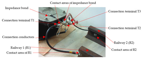
Figure 6.
Image of the electrical traction circuit elements used in the experiment.
The purpose of the experiment is to determine the temperature evolution of the terminal assembly of the impedance bond and conductor/connecting conductors (connection rope) for different connection modes (4 cases). To perform mathematical calculations of temperature evolution, it is necessary to correctly define the input data. Thus, it is considered a copper bar with a rectangular cross-section, having dimensions 30 × 8 × 100 [mm], which represents one of the three connecting terminals (T1, T2, T3) of a classic impedance bond [10]. On this terminal is connected, by means of a titanium screw size M8, one or two connecting conductors (made of steel or copper) which have a copper slipper mounted at the ends. The mechanical tightening between the bar and the connection rope was carried out with a torque wrench, at value of 30 [Nm].
For the definition of the analysis cases, the following ways of connecting the terminal of the impedance bond and the railway rail were considered:
- Connection by means of a copper connecting conductor. Its length is 0.65 [m], and the cross section is 50 [mm2]. The copper slippers at the ends of the connecting conductor have a diameter of d1 = 8 [mm], and the diameter d2 = 12 [mm], according to the standards, Figure 7 [10];
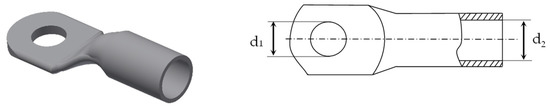 Figure 7. Copper slipper at the ends of the connecting conductors.
 - Connection by means of a steel connecting conductor. Its length is also 0.65 [m], but for this case the cross section is 78 [mm2]. The copper slippers at the ends of the connecting conductor have a diameter of d1 = 10 mm, and the diameter d2 = 12 mm, from Figure 7
- Connection by means of two connecting conductors made of steel. The dimensions of the conductors and slippers are the same as those defined for the second case
- Connection by means of two connecting conductors made of steel, having the particularity that one of the connecting conductors is not connected to the end from the railway rail. The dimensions for the connecting conductors and slippers are the same as those defined for the second case.
For each connection mode, the temperature evolution was studied at 3600 s from the moment of establishing the current through the circuit. For this purpose, it was considered to be transited through the assembly consisting of the impedance bond terminal and connection conductor a current of 100 [A]. Assembly was positioned in the ambient environment (air) at an ambient temperature of . For the material convection coefficient of thermal transmission, the value of 12 W/m2 °C was used, and for the thermal conductivity the value of 400 [W/m K] for copper and 40 [W/m K] for steel.
The value of the tightening torque in the contact was 30 [Nm], and for the hardness of the material was considered the value of 110 × 107 [N/m2], specific to copper [10].
For each individual case, the calculated assembly has been defined as being mechanically fixed at both ends, this being essential in the study of temperature evolution because due to the current transit through the current path mechanical changes also occur, and convergence to a solution requires this. The mechanical force of attachment being much higher than the contact force, having the value of 107 [N].
Being known the geometric dimensions of the assembly for each case, respectively of the current conductive path, the maximum overtemperatures (permanent regime) were calculated, for the contact area, with the relation:
where: a and b—represent the dimensions of the contact section; Inb—nominal current (100 [A]); ρ—the electrical resistivity of copper (1.6 × 10⁻⁸ [Ωm]), ks—coefficient of additional losses (1.05 ÷ 1.5) due to the proximity effect and contribution of the contact resistance as well as other thermal sources; αt—the global coefficient of heat transmission (which had values between 8 ÷ 12 [W/m2 °C]).
The temperatures of the contact areas were determined with the relation (57):
where the Uc voltage drop on the contact was measured for each case of connection with the Fluke P420 multimeter, and TP was measured as 21 [°C] = 294.15 K.
The temperatures of the contact areas were verified with the relation:
The thermal time constants T in the contact area, for each connection assembly separately, were calculated with the relation:
where: m—represents the mass of electrical contact; S—heat-exchange surface; c—specific heat.
For each mode of connection, considering that the resistivity does not change with the temperature, under the most unfavorable conditions, the following values: of the permanent regime overtemperatures; the overtemperatures determined at 3600 s; the electrical contacts temperatures; respectively for the thermal time constants and were listed in Table 4.
Table 4.
Mathematical determination of electrical contact parameters.
Figure 8 represents the heating curves of the contact areas corresponding to each connection mode, determined by relations (1) and (12).
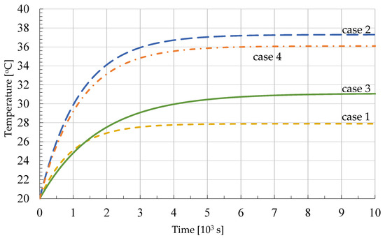
Figure 8.
Transient heating regime of the contact areas for each connection mode.
From the analysis of how the temperature evolves for each case, Figure 8, it is noticed that for the first case the permanent regime temperature is stabilized around 27.85 [°C]. For the other cases analyzed, it is observed that the value of the permanent regime temperature of the 1st case, did result a value closest to that of the 3rd case, when the temperature reaches the value of 31.06 [°C]. In the second and fourth cases the temperature in the contact zone will be higher, stabilized at 37.25 [°C] for the 2nd case and 36.06 [°C] respectively for the 4th one.
The differences in thermal time constants can be explained on account of the change in the mass and the heat-exchange surface, since the slipper of the steel connecting conductor rope is bigger than the one made of the copper. The main reason for copper conductor replacement with steel ones is in regard to vandalism avoiding and economical savings.
3.2. Performing the Simulation of Temperature Evolution
Further on, in order to simulate the connecting conductors’ temperature across the terminals of an impedance bond and the railway rails, by the use of COMSOL Multiphysics, version 5.6, finite element software.
The practical use of such a computer program involves the following steps:
- The preliminary settings selection: is achieved by choosing the way of defining the working conditions, the spatial dimension in which the study is intended to be carried out and the physical processes that are to be analyzed
- Definition of parameters and variables—for the analysis of the connecting conductors’ temperature evolution with different connection modes where defined parameters and variables for the 4 cases which were considered
- Geometric shape realization at scale by corresponding to each studied component. The computer program used allows the deactivation of some geometrical elements, thus being able to ignore certain parts of the structure of the studied components, Figure 9
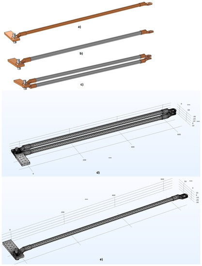 Figure 9. Geometry of the analyzed models: (a) a single copper conductor; (b) a single steel conductor; (c) two steel conductor mesh of the models; Mesh of the models: (d) two conductors; (e) single conductor.
- Definition of material parameters. The simulation software environment has a library of materials that includes the vast majority of materials used in electrical engineering, but also allows the definition of new materials. Table 5 is centralizing the considered material properties.
Table 5. Material parameters.
- Definition of boundary conditions. At this stage, the boundary conditions between the structural elements of the models and the environment in which they are located are established. For the connection modes of the impedance bond terminal and the current conductive path, border conditions have been defined for the electrical, thermal and mechanical properties. In order to maintain fixed positions of some constructive part of the models, throughout the simulation, the mechanical properties at their borders were defined. In order to obtain a convergent solution for the simulation were necessary to be de-fined fixed constrain for both ends of the models. Next, the border electrical properties, at the level of the contact surfaces, for an alternating current with a frequency of 50 Hz, having the value of 100 A, were defined. According to the electrical parameters defined, in the simulation, were considered as thermal input the power density. The border conditions for the thermal properties defined for the analyzed cases consisted in defining the surfaces that yield the heat flow, respectively those that are thermally insulated and declaring the value of the ambient temperature. In the case of thermal contact, the definition of the boundary conditions has been declared on the contact surfaces as in the case of electrical ones, adopting the sphere model. These border conditions cannot be fully in accordance with the system that is intended to be simulated, then approximations of the simulated models are required.
- Discretization of the model structural elements. The analysis of a models (as illustrated in Figure 9d,e) assumes a structure that can be divided into more or fewer nodes and elementary volumes. Vertices represent connecting points that maintain infinitesimal volumes in a unitary whole. For high precision, it is necessary to make it as smooth as possible, but this will make it difficult to achieve a convergence solution. For the proposed models was used “Free Tetrahedral” mesh type, which used 2,965,219 number of element (plus 95,042 internal DOFs). Thus, depending on the type of problem and the field of analysis, the most appropriate method of discretization must be defined in terms of the resources available. For several types of finite elements, at the border between them, continuity must be ensured, therefore, the transition from an area with fine discretization to one with less fine discretization, must be done progressively, not suddenly.
- Compilation of the model. At this stage, the effective numerical solution of the defined model will be achieved. The convergence of the solution is influenced by the size and number of finite elements, as well as the type of discretization chosen. The greater the number of infinitesimal elements, the closer the result gets to the real solution.
- Processing and interpretation of results. This last stage represents the phase of centralization of the results in tabular or graphic form. Thus, at this stage, it is possible to adjust the display of the results according to the ranges of interest, and it is also allowed to evaluate and comment on them.
By means of the simulation program using the finite elements analysis method, the temperature evolution was determined in the 4 connection modes specified above.
3.2.1. Case 1
In the first case scenario, it was considered that the connection between the terminal of the impedance bond and the railway rail is made by means of a copper connecting conductor that has at both ends a copper slipper. The tightening between the connecting conductor and the impedance bond terminal was made by a screw, according to Figure 9a. The screw tightening torque was 30 [Nm] and was equivalate in FEM as contact pressure defined by user, according to the cable connection standards in the electrical power installations [42].
Figure 10 shows the graphic image, generated by simulation, of the assembly considered in this case, from which it can be seen that the highest temperature value is recorded on the contact surface, the area corresponding to the overlap of the two components of the conductive path and is 27.3 [°C]. This is due to the additional presence of contact resistance (the electrical contact presence on the conductive path), which causes the temperature in this area to rise by about 7.3 [°C] from the ambient temperature at 3600 s. The value of the simulated overtemperature, compared to that obtained by calculations, Table 4, results in a difference lower by 0.41 [°C], which is due to the approximation assumptions considered in numerical modeling performing.
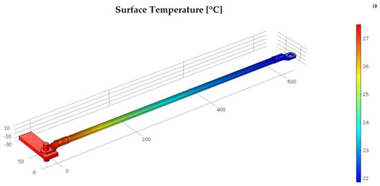
Figure 10.
Thermal stress of the connection made with a copper conductor.
3.2.2. Case 2
For the second case scenario, the connection between the impedance bond terminal and the railway consists of a steel connection conductor, which presents at both ends a copper slipper. And in this case the mechanical connection is made by means of a steel screw. The screw tightening torque was kept as in the first case, according to the standards. The electrical and thermal parameters change from the previous case because the properties of the materials differ, but the study conditions will remain unchanged. Thus, the temperature distribution on the surface of the assembly corresponding to this connection mode, at 3600 s, is shown in Figure 11.
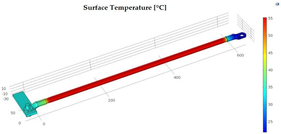
Figure 11.
Thermal stress of the connection made with a steel conductor.
From the analysis of the graphic image resulting from the simulation it can be inferred that in the second case the highest temperature value is recorded on the surface of the steel conductor and not on the surface of the contact area. So, after the 3600 s, according to the simulation results, the temperature on the surface of the contact area reaches around 35 [°C], while the temperature on the surface of the connecting conductor records the value of 55 [°C]. The ambient temperature was the same as for the first simulated case.
After comparing the graphic images resulting from the simulation, of the first two connection modes, Figure 10 and Figure 11, it is found that both the surface temperature on the connecting conductor and on the contact area surface is higher in the second case. Due to the electrical resistivity of steel, ρOl = 11.5 × 10⁻⁸ [Ωm], which is higher than copper, the steel conductor becomes an additional thermal source for the contact area.
The value of the simulated overtemperature, compared to that obtained by calculations, Table 4, results in a difference greater by 1.48 [°C]. As in the first case scenario, differences between the simulated and calculated temperature values appear.
3.2.3. Case 3
The connection, in this case scenario, between the impedance bond terminal and the railway is made with the help of two steel connecting conductors, which have at both ends a copper slipper. The dimensions of the connecting conductors, the mechanical connection and the tightening torque, the electrical and thermal parameters, respectively the study conditions remain the same as in the second case. The temperature distribution, on the surface of the assembly corresponding to this connection mode, at 3600 s, is given in Figure 12.
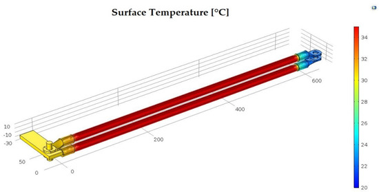
Figure 12.
Thermal stress of the connection made with two steel conductors.
From Figure 12 it is observed that the highest temperature value is recorded on the surface of the steel connecting conductors and not on the surface of the contact zone. Therefore, after the 3600 s, according to the simulation results, the temperature on the contact area surface reaches around 31.2 [°C], while the temperature on the surface of the connecting conductors, in the central area, records the value of 35 [°C].
If the graphic images resulting from the transient simulation for the last two connection modes (Figure 12 and Figure 13) are compared, it is found that in both cases the temperature on the surface of the connecting conductors is higher compared to that in the contact area. The value of the simulated overtemperature, compared to that obtained by calculations, Table 4, results in a difference lower than 1.54 [°C].
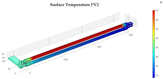
Figure 13.
Thermal stress of the connection made with two steel conductors, of which one is unconnected at one end.
Comparing, from the contact area temperature evolution point of view, the three analyzed cases, it can say that the first and third cases have close values of them, while for the second case the temperature evolution will be more pronounced. Therefore, from the thermal stress point of view, it is not preferable that the connection between the impedance bond terminal and the railway rail, to be made with a single steel connecting conductor.
In practice, the third way of connection is used, the contact area thermal stress is approximately equal to the first case scenario, since the cost of such a solution is lower with also having an increased mechanical strength.
3.2.4. Case 4
For the fourth case scenario, it is considered a particular situation in which the connection between the impedance bond terminal and the rail track is made by steel connecting conductors, in which one of them is not connected to the end to the railway rail. It was considered this situation because in operation the connecting conductors can be interrupted, due to mechanical vibrations, temperature evolution, etc. The dimensions of the connecting conductors, the mechanical connection and tightening torque, the electrical and thermal parameters, as well as the study conditions remaining the same as in the third case analyzed. Thus, the temperature distribution, on the surface of the assembly corresponding to this forth connection mode, at 3600 s, is shown in Figure 13.
By comparing the graphic images resulting from the transient simulation for the second and fourth cases scenarios (Figure 10 and Figure 13), it is found that for a current of the same value, the surface temperature of the connecting conductors has similar values in both cases. The value of the contact area overtemperature, obtained by simulation, has a value of 14.1 [°C] and the one of the calculations is 15.33 [°C], resulting in a difference of 1.23 [°C] between them.
Referring to the contact area surface temperature, we note that the temperature recorded for the fourth case from simulation result as 34.1 [°C], which is lower compared to the one from the second case, which was 35 [°C]. This is due to the fact that in the fourth case, two slippers are present in the contact area (of which is not active), in this case will have the role of a heatsink, compared to a single slipper in the second case scenario. The FEM analysis was used to estimate the temperature evolution by means of modern methods, and also to have a visual expression of the thermal phenomenon (the temperature variation along the models).
3.3. Monitoring of the Temperature Evolution by Means of Infrared Investigation
The validation of the conductive path simulation models was achieved through experimental tests consisting of their infrared thermographic investigations.
Infrared thermographic monitoring is one of the most modern methods of surveil-lance of temperature evolution, therefore, at present, it is used in the maintenance procedures applied in the electrical transformer substations, industrial applications and not only. The main advantage in such monitoring is that the temperature measurement is done remotely, without physical contact with the analyzed assembly. This allows for an investigation of a large area or perhaps even of the entire ensemble examined [35,36].
The monitoring carried out in the experiment was performed by means of the infrared thermographic investigation device (Flir T650sc). This was realized in order to determine the temperature evolution level of the contact between the impedance bond terminal and the slippers of the connecting conductors, at 3600 s from the moment of establishing the current through the circuit.
Figure 14 presents the wiring diagram used to monitor the temperature evolution of an alternating current of 100 A passed through the configuration. This configuration represents a portion of the power supply system return circuit of electric traction which uses a single-phase current with a frequency of 50 Hz and a voltage of 25 kV, commonly in Romanian railway electric traction [26,43]. The impedance bond’s terminals and the connecting conductors to the rail, used in the experiments, have the same dimensions, mechanical and electrical properties as those declared in the simulated models. Thus, in the experiments, as well as for simulation, the same four modes of connecting were considered. The ambient temperature at the time of the experiments was about 20 °C.
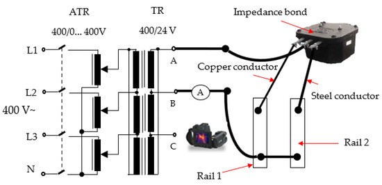
Figure 14.
Experimental setup electrical diagram.
Before performing the experimental thermal infrared investigation, corresponding to each case, contact resistance measurements were made using Micro Ohmeter RMO500A. The values of the contact resistances resulting from the measurements made, by transiting a test direct current in the amount of 100 A, are given in Table 6.
Table 6.
Contact resistance values measured for each case scenario.
Before performing the investigation, the thermal imaging camera is set according to the laboratory conditions [35,36].
The values of the adjustment parameters for obtaining the thermographic image were the following:
Ambient temperature: 20 [°C]
- Emissivity index: this parameter was set to the value of 0.95 corresponding to the emissivity of the conductor’s cables electric insulation
- Reflected temperature: set equal to the ambient temperature, 20 [°C]
- Relative air humidity: the value measured in the laboratory at the time of the experiment was 55%
- The distance from the camera lens to the investigated connection was 1 m
- The temperature range was selected between −30 ÷ 160 [°C]
- The temperature evolution for each of the four connection modes between the impedance bond terminal and the railway rail were monitored for 3600 s by transiting a current of 100 A, in order to validate the simulation models presented in previous section
3.3.1. Case 1 and 2
For the first and second cases, according to the electrical diagram from Figure 14, an infrared thermographic investigation was performed in order to monitor the temperature evolution for copper and steel connecting conductors. The tightening torque of the screws connecting the impedance bond terminal and the slipper of the connecting conductor was set in accordance with the connection standards, having the value of 30 [Nm]. After 3600 s from the moment of transiting the current, the thermographic image given in Figure 15 was obtained.
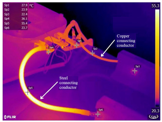
Figure 15.
Thermographic image of the copper and steel connecting conductors respectively.
The thermographic image obtained was processed, through Flir Tools software, to identify the temperatures recorded on each connecting conductor. Thus, corresponding to the Sp1 ÷ Sp3 points, the temperatures recorded for the copper connecting conductor are rendered, respectively for the Sp4 ÷ Sp6 points for the steel connecting conductor.
From the Figure 15 analysis, it is noticed that for the copper connecting conductor, the highest temperature is recorded on the connection area between the impedance bond terminal and the copper slipper, at point Sp1, having the value of 27.9 °C. While for the other two points the temperature registers a decrease, just as it was obtained from the simulation in case 1, Figure 10. The monitored temperature on the contact area surface is close in value to that obtained from the simulation of this type of connection (27.3 °C).
For the steel connecting conductor, the highest temperature is recorded on the conductor at point Sp5, having the value of 55.4 [°C], and on the connection terminal the value 36.1 [°C] corresponding to point Sp4 is recorded. From the simulation performed in case 2 (Figure 11) it results that the value resulted in the connection area is 35 [°C], therefore the value obtained from the thermographic investigation differs by 1.1 [°C]. So, for this case too, we can say that the simulation models are according to the real situation with a small deviation.
In conclusion, for these two cases, the thermal stress of the connections between the impedance bond terminals and the connecting conductors obtained from the simulation, are very close to the monitored values.
3.3.2. Case 3
For the third case, in which the connection between the impedance bond terminal and the railway rail is made by means of two steel connecting conductors, the thermographic image captured by the thermal imaging camera is shown in Figure 16.
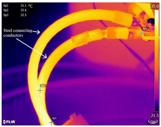
Figure 16.
Thermographic image of the two steel connecting conductors.
Analyzing Figure 16, it is observed that the temperature in the contact area, point Sp1, is 31.1 [°C], lower than the temperature on the steel conductors, points Sp2 and Sp3, which has values of approx. 33.5 [°C]. The experimentally recorded temperature distribution approaches the resulting values from the simulation of case 3, (which was 31.2 [°C] according to Figure 12).
For the value of the connection area temperature, corresponding to point Sp1, is observed a difference of 0.1 [°C] comparing to the value obtained from the simulation made for case 3. Thus, the experimental results validate the simulation model, and there is, however, a small temperature difference between them, which may be due to factors that were not considered in the simulation (e.g., the consideration of single wire conductors in the simulation, while in the experiment they were multi-wire conductors), respectively in the performance of experiments (the current value oscillated around 100 A during the tests, the ambient temperature did not remain constant at 20 °C).
3.3.3. Case 4
For the last case analyzed within the experiment, in which the connection mode be-tween the impedance bond terminal and the railway rail was made by two steel connecting conductors, having the particularity that one of the connecting conductors is not connected to the end towards the rail, the thermographic image from Figure 17 was obtained.
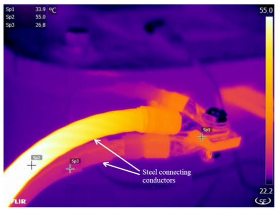
Figure 17.
Thermographic image of the two steel connecting conductors, of which one is unconnected at one end.
The temperature distribution obtained from the simulation of temperature evolution in case 4, Figure 13, is very close to that determined by the thermal imaging camera.
As in the third case, it is noticed that in the contact area, point Sp1, the temperature is 33.9 [°C], lower than the temperature on the active connecting conductor to the railway rail (the top one), marked by Sp2 point, which had the value of 55 [°C]. Thus, this time also, the temperature distribution resulting from the simulation (case 4) is close to that recorded by the thermal imaging camera.
Between the temperature value recorded by the thermal imaging camera at the connecting area, point Sp1, of 33.9 [°C] and the one obtained by simulation of 34.1 [°C], a difference of 0.2 [°C] is noted (Figure 13 and Figure 17).
For the four cases analyzed, the temperature values at 3600 s in the contact areas are centralized in Table 7.
Table 7.
Contact resistance values measured for each case scenario.
The temperature differences between the values obtained by the two methods (simulation and infrared investigation) are found in the range −0.2 ÷ +1.1 [°C]. Therefore, the experimental results obtained for the four connection modes considered, confirm the models used in the numerical simulation of thermal stress with an acceptable deviation.
4. Conclusions
The knowledge of the different situations that may occur in the operation of a railway traction supply system can be achieved by modeling it by means of equivalent schemes consisting of circuit elements (resistances, inductances, impedances etc.). The mathematical modeling of the main parameters within the analysis of these situations helps to determine as accurately as possible the values achieved during operation.
The temperature evolution of the conductive pathways in the return circuit are produced by the electrocaloric effect of the current circulating through them. The level of thermal stress also depends on the values of the contact resistances in the contact area. Thus, it was presented the possibility of evaluating the temperature evolution, of some connection modes from the return circuit, by modeling and numerically simulating them, the results being compared with those determined with the use of a thermal imaging camera, in order to validate them. The modeling and simulation of the thermal processes of the connecting conductors was performed with the COMSOL software environment that allows the easy determination, for example, of the values of the allowable currents, of the temperature evolution given by the nominal currents.
For modelling and numerical simulation, the following four ways of connecting the impedance bond terminal and the railway rail were considered:
- a copper connecting conductor with a cross section of 50 [mm2] (case 1)
- a steel connecting conductor with a cross-section of 78 [mm2] (case 2)
- two steel connecting conductors, each with a cross-section of 78 [mm2] (case 3)
- two steel connecting conductors having the particularity that one of the connecting conductors is not connected at one end (case 4)
By analyzing the numerical results, obtained at 3600 s from the moment of establishing the current through the circuit, the following were observed:
- higher temperatures in the contact area than those obtained on the connecting conductor surface, in the first case considered
- for the connection modes considered in cases 2, 3 and 4, the temperatures in the contact area are lower compared to those on the surface of the steel connecting conductors
- the surface temperatures distribution of the conductive path differs for the four analyzed cases
- more pronounced thermal stress for the second mode of connection compared to the others
The validation of the models made for the simulation of the conductive paths temperature from the return circuit was achieved through experimental tests in the laboratory.
The experimental results gave validity to the simulated thermal models of the conductive path, the deviations being below ±1.5 °C. By comparing the numerical results of the simulation with those obtained from thermographic recordings with the thermal imaging camera, it is possible to identify what needs to be modified in order to improve the simulation thermal models.
5. Patents
Adam M., Munteanu A., Pancu C.M., Andrusca M., “Method and system for locating the faulty sector in power supply installations in railway traction”, no. a 00936, 2018, Romania.
Adam M., Munteanu A., Pancu C.M., Andrusca M., “Method and apparatus for monitoring and diagnosis of impedance bond”, Request patent no. a 00233, 2017, Romania.
Author Contributions
Conceptualization, A.D., M.A. (Maricel Adam), M.A. (Mihai Andrusca); methodology, A.D., M.A. (Maricel Adam), M.A. (Mihai Andrusca); software, A.D., M.D.; validation, A.D., M.A. (Maricel Adam), M.A. (Mihai Andrusca), G.G.; formal analysis, A.D., M.A. (Maricel Adam), M.A. (Mihai Andrusca), G.G.; investigation, A.D., M.A. (Maricel Adam), M.A. (Mihai Andrusca); resources, A.D., M.A. (Maricel Adam), M.A. (Mihai Andrusca); data curation, A.D., M.A. (Maricel Adam), M.A. (Mihai Andrusca); writing—original draft preparation, A.D., M.A. (Maricel Adam), M.A. (Mihai Andrusca), M.D.; writing—review and editing, A.D., M.A. (Maricel Adam), M.A. (Mihai Andrusca), G.G., M.D; visualization, A.D. and S.R.; supervision, A.D., M.A. (Maricel Adam), M.A. (Mihai Andrusca) and S.R.; funding acquisition, A.D., M.A. (Maricel Adam), M.A. (Mihai Andrusca). All authors have read and agreed to the published version of the manuscript.
Funding
This work was supported by “Publications” an internal grant of the Technical University “Gheorghe Asachi” of Iasi (TUIASI), financed by contract no GI/P 15/2021.
Institutional Review Board Statement
Not applicable.
Informed Consent Statement
Not applicable.
Data Availability Statement
Not applicable.
Conflicts of Interest
The authors declare no conflict of interest.
References
- Vatau, D.; Iliasa, F.M.F.; Renghea, S.; Oros, C. A Didactic Method for Assessing the Influence of the Electromagnetic Field on the Environment. Procedia Soc. Behav. Sci. 2015, 191, 50–55. [Google Scholar] [CrossRef][Green Version]
- Pedersen, C.O.; Fisher, D.E.; Liesen, R.J. Development of a Heat Balance Procedure for Calculating Cooling Loads. ASHRAE Trans. 1997, 103, 459–468. [Google Scholar]
- Bauml, T.; Dvorak, D.; Frohner, A.; Simic, D. Simulation and Measurement of an Energy Efficient Infrared Radiation Heating of a Full Electric Vehicle. In Proceedings of the 2014 IEEE Vehicle Power and Propulsion Conference (VPPC), Coimbra, Portugal, 27–30 October 2014; pp. 1–6. [Google Scholar]
- Adam, M.; Baraboi, A. Echipamente Electrice (Electrical Equipment) Vol. 1-Gh; Asachi Publishing House: Iasi, Romania, 2002; pp. 143–167. [Google Scholar]
- Dragomir, A.; Adam, M.; Andruşcă, M.; Burlică, R.; Micu, M.B.; Patrichi, S. Simulating Electrical Connections in Terms of Thermal Stresses. In Proceedings of the 11th International Conference and Exposition on Electrical and Power Engineering—EPE, Iasi, Romania, 18–19 October 2018; pp. 361–366. [Google Scholar]
- Andruşcă, M.; Adam, M.; Burlică, R.; Munteanu, A.; Dragomir, A. Considerations regarding the influence of contact resistance on the contacts of low voltage electrical equipment. In Proceedings of the 9th International Conference and Exposition on Electrical and Power Engineering—EPE, Iasi, Romania, 20–22 October 2016; pp. 123–128. [Google Scholar]
- Liu, G.; Guo, D.; Wang, P.; Deng, H.; Hong, X.; Tang, W. Calculation of Equivalent Resistance for Ground Wires Twined with Armor Rods in Contact Terminals. Energies 2018, 11, 737. [Google Scholar] [CrossRef]
- Adam, M.; Baraboi, A. Echipamente Electrice (Electrical Equipment) Vol. 2-Gh; Asachi Publishing House: Iasi, Romania, 2002; pp. 124–136. [Google Scholar]
- Gatzsche, M.; Lücke, N.; Großmann, S.; Kufner, T.; Hagen, B.; Freudiger, G. Electric-thermal performance of contact elements in high power plug-in connections. In Proceedings of the 60th Holm Conference on Electrical Contacts (Holm), New Orleans, LA, USA, 12–15 October 2014; pp. 1–8. [Google Scholar]
- De Souza, R.T.; Da Costa, E.G.; De Oliveira, A.C.; De Sousa, W.T.; De Morais, C.M. Characterization of contacts degradation in circuit breakers through the dynamic contact resistance. In Proceedings of the Transmission & Distribution Conference and Exposition-Latin America (PES T&D-LA), Medellin, Colombia, 10–13 September 2014; pp. 1–6. [Google Scholar]
- Dragomir, A.; Adam, M.; Pancu, C.M.; Andruşcă, M.; Pantelimon, R. Monitoring of long term thermal stresses of electrical equipment. Sci. Bull. Ser. C 2015, 77, 245–253. [Google Scholar]
- Stąsiek, J.; Stąsiek, A.; Szkodo, M. Modeling of Passive and Forced Convection Heat Transfer in Channels with Rib Turbulators. Energies 2021, 14, 7059. [Google Scholar] [CrossRef]
- Aly, E.H.; Roșca, A.V.; Roșca, N.C.; Pop, I. Convective Heat Transfer of a Hybrid Nanofluid over a Nonlinearly Stretching Surface with Radiation Effect. Mathematics 2021, 9, 2220. [Google Scholar] [CrossRef]
- Zipunova, E.; Savenkov, S. On the Diffuse Interface Models for High Codimension Dispersed Inclusions. Mathematics 2021, 9, 2206. [Google Scholar] [CrossRef]
- Kim, H.; Kim, J. Numerical Study on Optics and Heat Transfer of Solar Reactor for Methane Thermal Decomposition. Energies 2021, 14, 6451. [Google Scholar] [CrossRef]
- Ramadan, A.N.; Jing, P.; Zhang, J.; Zohny, H.N.E.-D. Numerical Analysis of Additional Stresses in Railway Track Elements Due to Subgrade Settlement Using FEM Simulation. Appl. Sci. 2021, 11, 8501. [Google Scholar] [CrossRef]
- Song, W.; Jiag, Z.; Staines, M.; Vimbush, S.; Badcock, R.; Fang, J. AC loss calculation on a 6.5 MVA/25 kV HTS traction transformer with hybrid winding structure. IEEE Trans. Appl. Supercond. 2020, 30, 1–5. [Google Scholar] [CrossRef]
- Roy, P.; Bourgault, A.J.; Towhidi, M.; Song, P.; Li, Z.; Mukundan, S.; Rankin, G.; Kar, N.C. An algorithm for effective design and performance investigation of active cooling system for required temperature and torque of pm traction motor. IEEE Trans. Magn. 2021, 57, 1–7. [Google Scholar] [CrossRef]
- Li, S.; Sarlioglu, B.; Jurkovic, S.; Patel, N.R.; Savagian, P. Analysis of Temperature Effects on Performance of Interior Permanent Magnet Machines for High Variable Temperature Applications. IEEE Trans. Ind. Appl. 2017, 53, 4923–4933. [Google Scholar] [CrossRef]
- Feng, D.; Lin, S.; He, Z.; Sun, X.; Wang, Z. Failure Risk Interval Estimation of Traction Power Supply Equipment Considering the Impact of Multiple Factors. IEEE Trans. Transp. Electrif. 2017, 4, 389–398. [Google Scholar] [CrossRef]
- Muñoz-Condes, P.; Gomez-Parra, M.; Sancho, C.; San Andres, M.A.G.; González-Fernández, F.J.; Carpio, J.; Guirado, R. On Condition Maintenance Based on the Impedance Measurement for Traction Batteries: Development and Industrial Implementation. IEEE Trans. Ind. Electron. 2013, 60, 2750–2759. [Google Scholar] [CrossRef]
- Jang, H.; Kim, H.; Nam, D.-W.; Kim, W.-H.; Lee, J.; Jin, C. Investigation and Analysis of Novel Skewing in a 140 kW Traction Motor of Railway Cars That Accommodate Limited Inverter Switching Frequency and Totally Enclosed Cooling System. IEEE Access 2021, 9, 121405–121413. [Google Scholar] [CrossRef]
- Zhang, Y.; Wei, X.; Fan, X.; Wang, K.; Zhuo, R.; Zhang, W.; Liang, S.; Hao, J.; Liu, J. A Prediction Model of Hot Spot Temperature for Split-Windings Traction Transformer Considering the Load Characteristics. IEEE Access 2021, 9, 22605–22615. [Google Scholar] [CrossRef]
- Whitt, R.; Huitink, D.; Emon, A.; Deshpande, A.; Luo, F. Thermal and Electrical Performance in High-Voltage Power Modules with Nonmetallic Additively Manufactured Impingement Coolers. IEEE Trans. Power Electron. 2020, 36, 3192–3199. [Google Scholar] [CrossRef]
- Nategh, S.; Zhang, H.; Wallmark, O.; Boglietti, A.; Nassen, T.; Bazant, M. Transient Thermal Modeling and Analysis of Railway Traction Motors. IEEE Trans. Ind. Electron. 2018, 66, 79–89. [Google Scholar] [CrossRef]
- Andrusca, M.; Adam, M.; Dragomir, A.; Lunca, E. Innovative Integrated Solution for Monitoring and Protection of Power Supply System from Railway Infrastructure. Sensors 2021, 21, 7858. [Google Scholar] [CrossRef] [PubMed]
- Martínez, J.; Riba, J.-R.; Moreno-Eguilaz, M. State of Health Prediction of Power Connectors by Analyzing the Degradation Trajectory of the Electrical Resistance. Electronics 2021, 10, 1409. [Google Scholar] [CrossRef]
- Wu, Y.; Ruan, J.; Gong, Y.; Long, M.; Li, P. Contact Resistance Model and Thermal Stability Analysis of Bolt Structure. IEEE Trans. Components. Packag. Manuf. Technol. 2018, 9, 694–701. [Google Scholar] [CrossRef]
- Nituca, C. Thermal analysis of electrical contacts from pantograph–catenary system for power supply of electric vehicles. Electr. Power Syst. Res. 2013, 96, 211–217. [Google Scholar] [CrossRef]
- Zhang, P.; Li, W.; Yang, K.; Feng, Y.; Cheng, P.; Wang, C.; Zhan, H. Condition estimate of contacts of current-carrying conductor in GIS based on the FEM calculation of temperature field. In Proceedings of the 2015 3rd International Conference on Electric Power Equipment—Switching Technology (ICEPE-ST), Busan, Korea, 25–28 October 2015; pp. 69–73. [Google Scholar]
- Szulborski, M.; Łapczyński, S.; Kolimas, L.; Zalewski, D. Transient Thermal Analysis of the Circuit Breaker Current Path with the Use of FEA Simulation. Energies 2021, 14, 2359. [Google Scholar] [CrossRef]
- Dragomir, A.; Adam, M.; Andrusca, M.; Atanasoaei, M.; Rusu, O.; Miron, A.; Iamandi, A. Aspects Regarding the Infrared Monitoring of Electrical Equipment Temperature. In Proceedings of the 11th International Conference and Exposition on Electrical and Power Engineering—EPE, Iasi, Romania, 22–23 October 2020. [Google Scholar]
- Andrusca, M.; Adam, M.; Dragomir, A.; Lunca, E.; Seeram, R.; Postolache, O. Condition Monitoring System and Faults Detection for Impedance Bonds from Railway Infrastructure. Appl. Sci. 2020, 10, 6167. [Google Scholar] [CrossRef]
- Braunovic, M. Effect of connection design on the contact resistance of high power overlapping bolted joints. IEEE Trans. Components Packag. Technol. 2002, 25, 642–650. [Google Scholar] [CrossRef]
- Orlove, G.; Willis, J. Infrared Thermometer Emissivity Tables; Flir Research and Science: Goleta, CA, USA, 2015. [Google Scholar]
- Lizak, F.; Kolcun, M. Improving reliability and decreasing losses of electrical system with infrared thermography. Acta Electrotech. Et. Inform. 2008, 8, 60–63. [Google Scholar]
- Pop, I.; Roşca, N.C.; Roşca, A.V. Additional results for the problem of MHD boundary-layer flow past a stretching/shrinkingsurface. Int. J. Numerical Methods Heat. Fluid. Flow 2016, 26, 2283–2294. [Google Scholar] [CrossRef]
- Sundar, L.S.; Sharma, K.V.; Singh, M.K.; Sousa, A. Hybrid nanofluids preparation, thermal properties, heat transfer and friction factor-A review. Renew. Sustain. Energy Rev. 2017, 68, 185–198. [Google Scholar] [CrossRef]
- Garroni, A.; Marziani, R.; Scala, R. Derivation of a Line-Tension Model for Dislocations from a Nonlinear Three-Dimensional Energy: The Case of Quadratic Growth. SIAM J. Math. Anal. 2021, 53, 4252–4302. [Google Scholar] [CrossRef]
- Dragomir, A.; Adam, M.; Andrusca, M.; Astanei, D.G.; Andrusca, L.; Dumitrescu, C. About Some Connection Modes of the Current Conducting Paths. In Proceedings of the 10th International Conference and Exposition on Electrical and Power Engineering—EPE, Iasi, Romania, 18–19 October 2018; pp. 357–360. [Google Scholar]
- Hong, W.; Pitike, K.C. Modeling Breakdown-resistant Composite Dielectrics. Procedia IUTAM 2015, 12, 73–82. [Google Scholar] [CrossRef]
- Hong, Z.; Campbell, A.M.; Coombs, T.A. Numerical solution of critical state in superconductivity by finite element software. Supercond. Sci. Technol. 2006, 19, 1246–1252. [Google Scholar] [CrossRef]
- Schlösser, R.; Schmidt, H.; Leghissa, M.; Meinert, M. Development of high-temperature superconducting transformers for railway applications. IEEE Trans. Appl. Supercond. 2003, 13, 2325–2330. [Google Scholar] [CrossRef]
- Cozman, F.G. Graphical models for imprecise probabilities. Int. J. Approx. Reason. 2005, 39, 167–184. [Google Scholar] [CrossRef]
- Langan, P.E. The art of impedance testing. In Proceedings of the 1999 IEEE/-IAS/PCA Cement Industry Technical Conference, Roanoke, VA, USA, 11–15 April 1999; pp. 121–129. [Google Scholar]
- Yolacan, E.; Guven, M.K.; Aydin, M.; El-Refaie, A.M. Modeling and Experimental Verification of an Unconventional 9-Phase Asymmetric Winding PM Motor Dedicated to Electric Traction Applications. IEEE Access 2020, 8, 70182–70192. [Google Scholar] [CrossRef]
- Skillen, A.; Revell, A.; Iacovides, H.; Wu, W. Numerical prediction of local hot-spot phenomena in transformer windings. Appl. Therm. Eng. 2012, 36, 96–105. [Google Scholar] [CrossRef]
- Cengel, Y.; Ghajar, A.J. Heat and Mass Transfer: Fundamentals and Applications; McGraw-Hill: New York, NY, USA, 2014; pp. 134–156. [Google Scholar]
- Hettegger, M.; Streibl, B.; Biro, O.; Neudorfer, H. Measurements and Simulations of the Convective Heat Transfer Coefficients on the End Windings of an Electrical Machine. IEEE Trans. Ind. Electron. 2011, 59, 2299–2308. [Google Scholar] [CrossRef]
- Slade, P.G. Electrical Contacts Principles and Application, 2nd ed.; CRC Press Taylor and Francis Group: London, UK, 2014; pp. 249–298. [Google Scholar]
Publisher’s Note: MDPI stays neutral with regard to jurisdictional claims in published maps and institutional affiliations. |
© 2021 by the authors. Licensee MDPI, Basel, Switzerland. This article is an open access article distributed under the terms and conditions of the Creative Commons Attribution (CC BY) license (https://creativecommons.org/licenses/by/4.0/).