Article

Multi-Objective Artificial Bee Colony Algorithm with Minimum Manhattan Distance for Passive Power Filter Optimization Problems

Department of Electrical Engineering, National Taiwan University of Science and Technology, Taipei 10607, Taiwan
*
Author to whom correspondence should be addressed.
Mathematics 2021, 9(24), 3187; https://doi.org/10.3390/math9243187
Submission received: 26 October 2021 / Revised: 6 December 2021 / Accepted: 7 December 2021 / Published: 10 December 2021
(This article belongs to the Special Issue Metaheuristic Algorithms)

Abstract

:
Passive power filters (PPFs) are most effective in mitigating harmonic pollution from power systems; however, the design of PPFs involves several objectives, which makes them a complex multiple-objective optimization problem. This study proposes a method to achieve an optimal design of PPFs. We have developed a new multi-objective optimization method based on an artificial bee colony (ABC) algorithm with a minimum Manhattan distance. Four different types of PPFs, namely, single-tuned, second-order damped, third-order damped, and C-type damped order filters, and their characteristics were considered in this study. A series of case studies have been presented to prove the efficiency and better performance of the proposed method over previous well-known algorithms.

1. Introduction

1.1. Background

Nonlinear loads such as rectifiers, power converters, computers, televisions, and a multitude of others have become indispensable in the modern world. However, they have some disadvantages owing to their application, and harmonics are one of them [1,2]. Harmonics in power systems is a major and typical problem that occurs because of the distortion in the current and voltage waveforms that use nonlinear loads [1,3,4,5]. These harmonics cannot be ignored because of their harmful effects on the system, that is, power loss, equipment malfunctioning, device deterioration, and other damages [6,7,8,9,10,11,12]. Various mitigation techniques have been proposed by researchers to eliminate or reduce these harmonics, some of which are reactors and chokes, power filters (PF), and higher pulse number converters. However, PF is still considered as the first choice among them. Generally, three types of PF are available in the applications for reducing harmonic pollution from the system. These are passive power filters (PPFs), active power filters (APFs), and hybrid power filters (HPFs). Some related studies have demonstrated the usefulness of PFs in reducing harmonics. Among all power filters, passive filters are commonly used because of their simple circuit structure, low cost, and flexibility [13,14,15].
The optimization algorithms are not only used for calculating the parameters of PPFs, but also for evaluating the sizing, sitting, type, number of PPFs [16,17,18,19], minimizing the initial investment costs [20], minimizing the harmonic distortion [21], and maximizing the reactive power compensation [22]. Therefore, the design of PPF problems involves multiple objectives with multiple constraints. Several methods have been proposed to design PFFs over the past two decades. J. C. Das developed a conventional trial-and-error-based method for designing PPFs [13]. When using the conventional trial-and-error-based method, it is difficult to obtain optimal solutions with time-consuming tasks. In recent years, heuristic optimization algorithms such as the genetic algorithm (GA) [16,23,24], particle swarm optimization (PSO) [17,19], and simulated annealing (SA) [25] have been used for PPF designs.
Other methods have been recently employed, and their results were investigated to design PPFs [26,27,28,29,30,31]. Badugu R. et al. developed a class topper optimization (CTO) for PPF design [26]. The detuning mechanisms that were employed were complex, which in turn made it difficult to achieve an optimal solution. Wang Y. et al. employed a tuning filtering method to achieve good results [27]. However, thorough an examination, tuning was still a limitation for the PPF design. A more advanced tuning method was used via a dynamic tuning passive filter (DTPF) and it is listed in [28]. Even though this method offers an efficient harmonic suppression, the need for value-range setting of the harmonic current coefficient cannot be ignored. In [29,30], research on harmonic mitigation was conducted using PSO. However, an unbalanced power system is a possibility, owing to the use of the weight sum method. In [31], a more recent method that uses teaching-learning-based optimization (TLBO) with Pareto optimality was developed. Although this method can perform well, the deployment of TLBO and Pareto to obtain the desired PPF design requires good integration practices between the external archive and fuzzy system for decision making.

1.2. Aim and Contributions

This study proposes a new multi-objective algorithm, based on the famous artificial bee colony (ABC) algorithm. ABC is a recently developed meta-heuristic algorithm that uses the foraging behavior of honey bees, that is, searching for a food source and selecting the best on the basis of nectar amount. The ABC algorithm was first introduced by Karaboga in 2005 [32] and its performance was evaluated in 2008 [33]. Although this algorithm has been applied to several optimization problems [34,35,36,37,38,39,40,41], no research focusing on the PPF design using the ABC algorithm either in a single-objective or multi-objective optimization domain is available in the literature. Therefore, a new multi-objective artificial bee colony (MOABC) algorithm has been proposed to solve the multi-objective problem as a PPF design. The weight sum method was used to simplify a multi-objective optimization problem into a single-objective optimization problem [18,19,23]. However, the weight sum method may cause an imbalance between objective functions. Therefore, Pareto optimality is introduced with MOABC to make the design of PPFs more efficient. Some research has shown the use of Pareto optimality to solve multi-objective problems [18,19,42]. In addition, an external archive was used to store all possible solutions [43,44,45,46,47,48]. In the experimental work, a series of case studies are presented to prove the efficiency and superiority of the proposed method. At first, the proposed method was compared with a previously well-known SA for three different cases. Secondly, the proposed method was compared with two other well-known algorithms, namely, the PSO and bat algorithm (BA), in terms of minimum Manhattan distance (MMD) results [49]. In each case, the results were in favor of the proposed method, demonstrating better performance and superiority over all the other methods mentioned previously.

1.3. Paper Organization

This remainder of this paper is organized as follows: Section 2 introduces the PPF design problem with their objectives and constraints; Section 3 explains the multiple objectives of the PPF design; Section 4 discusses the proposed algorithm, which is an original ABC algorithm, MOABC, and the implementation of the proposed method to the PPFs problem; Section 5 presents the experimental results; and Section 6 presents the conclusion.

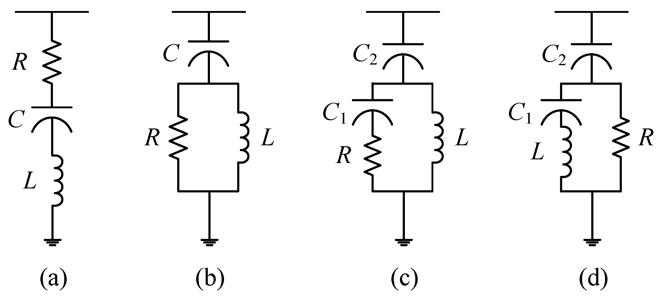
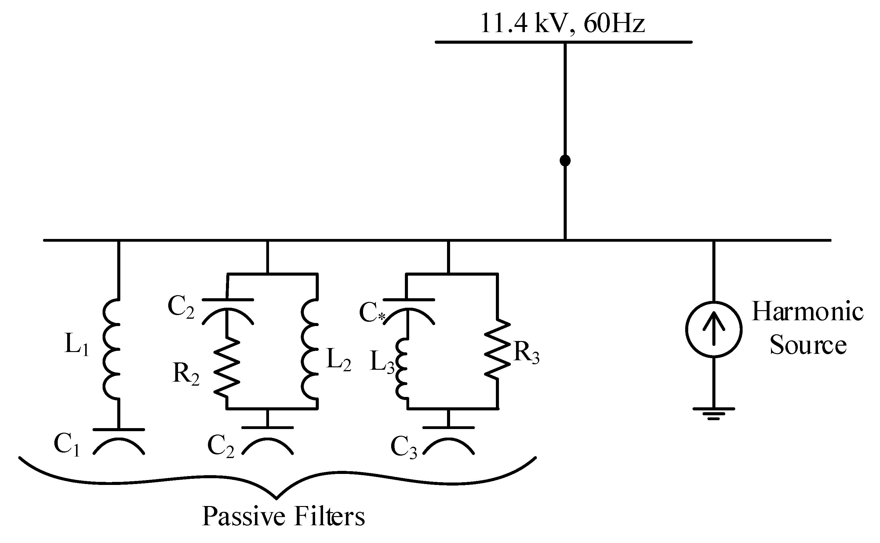
2. Passive Power Filters and Their Characteristics

Power filters are considered most effective in distribution systems for reducing harmonic pollution, owing to their low cost and simple design. Resistors, inductors, and capacitors are the passive elements of PPFs. Here, four types of PPFs were used, including a single-tuned (ST) filter, second-order damped (SD) filter, third-order damped (TD) filter, and C-type damped (CD) filter, as depicted in Figure 1. The harmonic impedances of the PPFs used in this study are listed in Table 1.

3. Problem Formulation

With the rapid development of new technology, new methods are being developed to improve power quality, and PPFs are one of them. Different types of PPFs are used to repress critical harmonics from the power system. From Figure 2a, we can see that the one-line diagram of a simple system is composed of PPFs, a power supply, and a nonlinear load. The point of common coupling (PCC) is the point where the generating facility is connected to the distribution system, and PPFs prevent it from generating harmonics. The simple system is composed of a power supply, passive filters, and nonlinear loads. Among them, the nonlinear load can be assumed as the harmonic source; the system network and the passive filter are regarded as the equivalent impedances, and the remaining linear loads can be ignored, owing to their large impedances. According to Figure 2b, the relationship between the system voltage and current can be obtained as follows:
V S h = Z F h · Z S h Z F h + Z s h I h ,
I S h = Z F h Z F h + Z S h I h ,
I F h = Z S h Z F h + Z S h I h ,
where h is the harmonic order; I h is assumed to be the harmonic current source; I F h and I S h are the harmonic currents through the filter and power supply terminal, respectively;   Z S h and Z F h are the system impedance and filter impedance, respectively.

3.1. Objective Functions

The design of PPFs involves several objectives such as minimizing the total harmonic distortion of voltage and current, installation cost, and maximizing fundamental reactive power compensation. Therefore, the design of PPFs is considered as a multi-objective optimization problem. The objectives of this study are discussed below:

3.1.1. Minimizing Total Harmonic Distortion of Current

The total harmonic distortion of the current is defined as,
F 1 = T H D I = ( h = 2 H | I h | 2 ) | I 1 | ,
where h is the harmonic, H is the highest harmonic order, | I 1 | is the rms of the fundamental current, and | I h | is the rms of the harmonic current with integer order.

3.1.2. Minimizing Total Harmonic Distortion of Voltage

The total harmonic distortion of the voltage is defined as follows:
F 2 = T H D V = ( h = 2 H | V h | 2 ) | V 1 | ,
where h is the harmonic, H is assumed to be the highest harmonic order, | V 1 | indicates the rms of the fundamental part of the voltage, and | V h | is regarded as the rms value of the harmonic voltage with integer order.

3.1.3. Minimizing Initial Investment Cost

The overall investment cost of a PPF includes the installation cost, power loss, materials, and maintenance costs. The cost is evaluated through the linear combination of each element (R, L, and C), which is used in designing the PPF with a weighting coefficient for each element. The initial investment cost can be expressed as follows:
F 3 = I C = m = 1 4 α m n = 1 X m ( k 1 R m n + k 2 L m n + k 3 C m n ) ,
where m is the type of filter and X m is the number of filters of type m . R m n , L m n , and C m n are the resistance, inductance, and capacitance of the n -th filter of type m , respectively; k 1 , k 2 , and k 3 are the cost-weighting coefficients; α m is considered as the set number coefficient for the m-type filter [25].

3.1.4. Maximizing Total Fundamental Reactive Power Compensation

PPFs are not only used to solve the problems of harmonic pollution, but also to compensate for the power factor. The total fundamental reactive power produced by the filters is expressed as,
Q F = m = 1 4 n = 1 X m Q F m n ,
where Q F m n is the fundamental reactive power produced by the n-th filter of the m-th type. Because all of the abovementioned objectives concern finding the minimum value, the objective function can be rewritten as,
F 4 = Q m a x Q F ,
where Q m a x is the maximum reactive power compensation.

3.2. Constraints

In constraint optimization problems, every objective has some limitations, called constraints. The four main objectives have been discussed so far, and their constraints are provided below.

3.2.1. Total Harmonic Distortion

The total harmonic distortions of currents and voltages are restricted by
g 1 = T H D I T H D I , m a x ,
g 2 = T H D V T H D V , m a x ,
where T H D I , m a x and T H D V , m a x are the maximum restriction values for the total harmonic distortions of the currents and voltages, respectively.

3.2.2. Individual Harmonic Distortion

The individual harmonic distortions for each order harmonic component are restricted by
g 3 = H D I h | I S h | | I S 1 | H D I h , m a x ,
g 4 = H D V h | V S h | | V S 1 | H D V h , m a x ,
where H D I h , m a x and H D V h , m a x are the maximum restriction values for the harmonic current and voltage at the h-th order, respectively.

3.2.3. Total Fundamental Reactive Power Compensation

PPFs can effectively improve the power factor of the system. However, overcompensation may cause voltage instability and increases the power loss. Therefore, the limitation of the total fundamental reactive power can be expressed as follows:
g 5 = Q m i n Q F Q m a x ,
where Q m i n and Q m a x are the minimum and maximum reactive power compensations, respectively.

4. Proposed Algorithm

4.1. Single-Objective Artificial Bee Colony Algorithm

ABC is a heuristic optimization algorithm. The original ABC algorithm was first developed by Karaboga in 2005 [32]. Initially, it was proposed to handle unconstrained problems [33] but it was later modified to solve the constrained optimization problem [37]. The foraging behavior of honey bees was used to solve optimization problems. ABC is a straightforward and fast-converging algorithm with fewer parameters required, which constitutes its unique nature.
ABC is composed of the following three classes of bees: employed, onlooker, and scout bees. In the first class, the employed bees travel to search for food source positions randomly. After reaching the food source, it produces a new solution and compares it with the old one using the greedy selection procedure. Thereafter, they exchange information regarding the food source, such as path, profitability, and nectar quantity, to the onlooker bees in the dance area of the hive by waggle dancing. Therefore, the onlooker bees are assigned to choose the food source position based on the probability proportionate to the quality of the food source and to update the new one. The higher the fitness, the greater the chances to be selected. Furthermore, the greedy selection procedure is performed for the onlooker bees, indicating new and old food sources to maintain a better food source with high nectar quantity for the next generation.
Consequently, a good quality food source is provided rather than a bad one with low nectar quantity. After a certain number of trials, if the food source cannot be improved, it will be rejected and replaced by a randomly selected food source. The employed bee associated with that food position abandons it and become a scout bee. The scout bee then starts its food-source search cycle randomly. The possible solution represents the food source position, and the fitness function addresses the nectar amount of that particular food position. The number of employed bees (or onlooker bees) is proportional to the position of the food source.
Three steps are involved in each cycle of the ABC algorithm. First, the possible food-source positions and their nectar amounts are determined by the employed bee, who shares their knowledge with the onlooker bee. Second, onlookers select a food source using a probabilistic approach. Third, the scout bees are initialized and sent to the entirety of the new food-source positions. During the search process, the best solution obtained is stored in the external archive.
The main steps of the ABC algorithm are listed below:
  • Initialization: Initialization is the first step in which the population denoted by P of N S solution (food source position) is initialized. Moreover, each solution x m n ( m = 1 ,   2 ,   3 ,   ,   N S ; n = 1 ,   2 ,   3 ,   , D ) is supposed to be a D -dimensional vector, where N S is denoted as the number of onlookers/employed bees and D is the number of parameters for optimization.
  • Employed bee phase: In the starting phase, the employed bees are sent to identify the positions of food sources and update the feasible food sources in the memory. The memory is updated to produce a feasible candidate using (14) [32].
    v m n = x m n + m n ( x m n x k n ) , n { 1 ,   2 ,   3 ,   ,   D } ,   k { 1 ,   2 ,   3 ,   ,   N S }     k i ,
    where v m n is considered as the new optimal position of the food source produced by the employed bee and m n is supposed to be a random number within the range of [−1, 1] to modify the production of neighboring food sources near x m n and compare the positions of the two food sources.
  • Onlooker bee phase: After evaluating the quality (fitness) of the food source position in the memory using (15), the onlooker bee chooses the best position of the food source, based on the probability proportional to the quality of food source through (16) [33]. Update the feasible candidate by the onlooker bees using (14).
    f i t m = { 1 / ( 1 + F m )                           i f ( F m 0 ) 1 + abs ( F m )                         i f ( F m < 0 ) ,
    p m = f i t m i = 1 N S f i t i ,
    where F m is considered as the objective function value, f i t m is supposed to be the measure of the fitness value of the solution m proportional to the nectar quantity of the food source, and N S is the number of employed/onlooker bees.
  • Scout bee phase: If the food source cannot be improved via a limited number of trials, then the food source is discarded. In addition, the associated employed bee becomes a scout bee to randomly search for a new source of food using (17) [32,33].
    x m n = x m i n n + rand [ 0   , 1 ] ( x m a x n x m i n n ) ,
    where x m i n n and x m a x n are the lower and upper bounds of each variable for the search scope, respectively. Here, in every x m n vector, the range [ x m i n , x m a x ] is the boundary of each component so that the scout bee does not leave the search space.
  • Memory update: Save the best position of food source found so far.
  • Termination check: Finally, a check is performed as to whether the termination condition is reached; if yes, the algorithm is terminated, and the final solutions are reported; otherwise, return to the starting search phase, that is, the employed bee phase.

4.2. Multi-Objective Artificial Bee Colony Algorithm

ABC was initially proposed to solve single-objective optimization problems. However, most engineering problems are multi-objective problems; therefore, the ABC algorithm was later extended to solve multi-objective optimization problems. There are several approaches that can be used to extend a single-objective algorithm to a multi-objective algorithm. In [34], the ABC algorithm was applied to solve the fixed-point problem in mathematics. In [40], a Pareto-based ABC was proposed using a crowding distance archive in NSGA-II to store non-dominated solutions, commonly used in multi-objective algorithms. Several other publications are also available in which the ABC algorithm is used to solve multi-objective problems [36,38,39,40,41]. In [48], a different Pareto dominance approach was incorporated into PSO. This algorithm used an external archive to store the Pareto solution that was used to enrich the exploratory capabilities. The approach using an external archive provides better performance than approaches using a crowding distance archive. Some data indicate that the ABC algorithm can maintain an adequate balance between exploitation (employed bee phase and onlooker bee phase) and exploration (scout bee phase) [50,51]. Therefore, ABC has a simple concept, good balance, fast convergence, and fewer control parameters, making the ABC algorithm attractive to many researchers. In this study, a modified ABC algorithm with Pareto optimality and an external archive has been proposed to optimize the design of the PPF more efficiently.

4.2.1. Pareto Optimality

In multi-objective optimization problems, a conflict exists between solutions. In other words, one solution cannot minimize or maximize all objectives simultaneously. Therefore, Pareto optimality is used.
The set of objective vectors of the Pareto optimal set is called the Pareto front. The search space of decision variables comprises several hypercubes to obtain an appropriate Pareto front.
Suppose a multi-objective optimization problem, in which minimization of an objective function is required. That is,
Minimize   F j ( x ¯ )   ( j = 1 ,   2 ,   ,   n F ) ,
subject to
g k ( x ¯ ) 0   ( k = 1 ,   2 ,   ,   n g ) ,
h l ( x ¯ ) = 0   ( l = 1 ,   2 ,   ,   n h ) ,
where x ¯ and F j ( x ¯ ) are the vector of decision variables and an objective function, respectively; n F is the number of objective functions; g k ( x ¯ ) and h l ( x ¯ ) are the inequality and equality constraints, respectively; and n g and n h represent the number of inequality and equality constraints, respectively.
x ¯ = [ x 1 ,   x 2 ,   ,   x n ] t ,   x ¯ Ω S ,
a region where a decision variable x ¯ satisfies all the constraints is called a feasible region and is denoted by set Ω and S is assumed as a search space.
Suppose F 1 ( x ¯ 1 ) and F 2 ( x ¯ 2 ) are two objective functions:
F m ( x ¯ 2 ) F m ( x ¯ 1 )     m { 1 ,   2 ,   3 ,   ,   k }   and
F m ( x ¯ 2 ) < F m ( x ¯ 1 )     m { 1 ,   2 ,   3 ,   ,   k } .
If a decision variable x ¯ 2 Ω and its function F m ( x ¯ 2 ) dominates over all other F m ( x ¯ ) functions for each x ¯ Ω , then the vector decision variable x ¯ 2 belongs to the non-dominated solution.

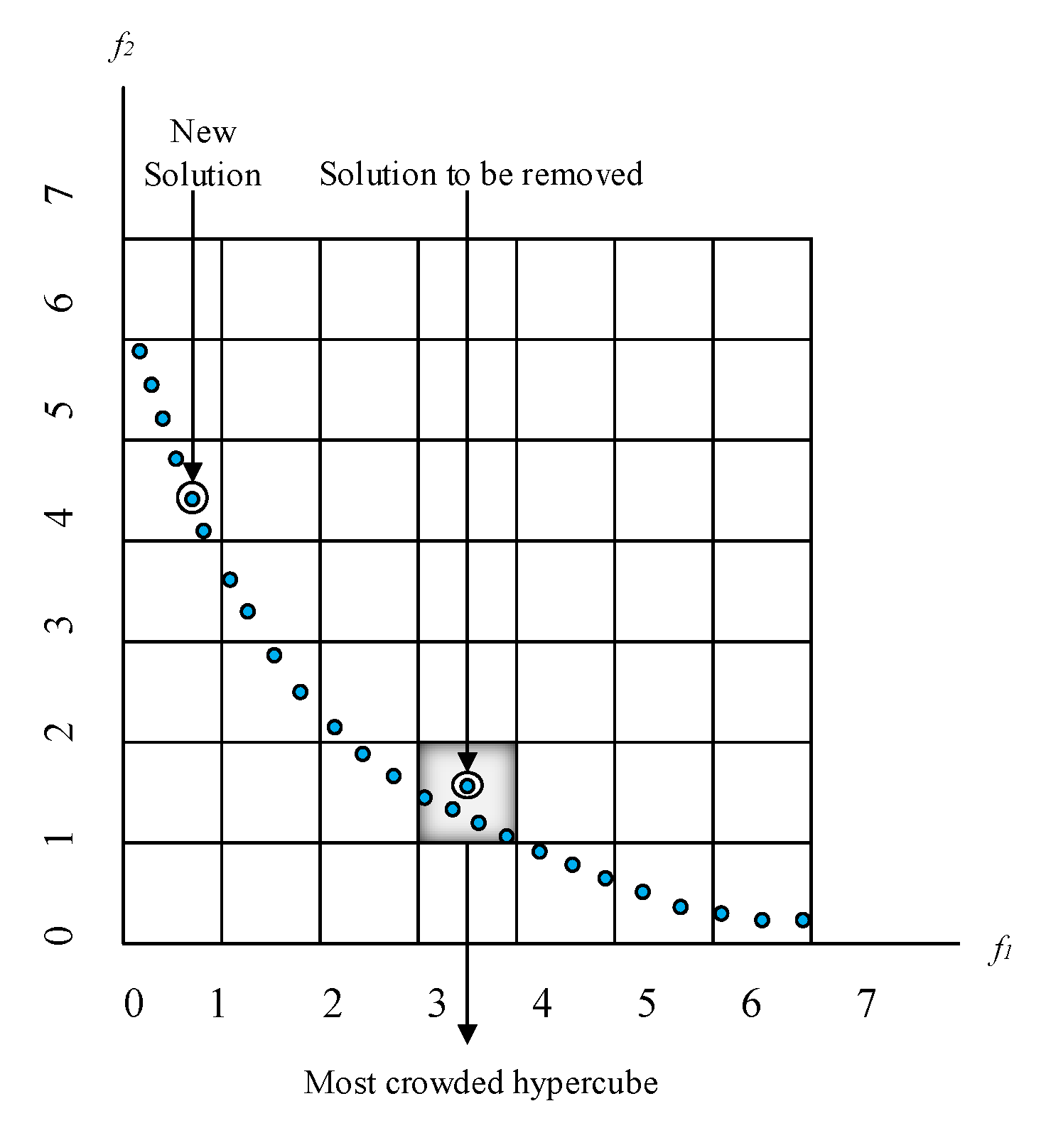
4.2.2. External Archive

Multi-objective problems involve non-dominated solutions. Several non-dominated solutions are produced in each iteration; therefore, it is necessary to store these solutions. For storing purposes, an external archive was used by researchers using PSO and an evolutionary algorithm (EA). The size of the external archive was restricted and updated during each iteration. In practice, a size of 100 solutions was used [48]. The storing solution process is simple as the solution is stored if, and only if, it is a non-dominated solution within the archive.
Figure 3 graphically depicts the concept of the selection and removal of the solution from the external archive, as listed in [52]. If the solution is out of constraints (infeasible), it will be rejected. If the solution comes under all constraints (feasible) and the archive is not full, then it will be stored in the archive. If the archive is full, then the feasible solution will be compared with other solutions. If it dominates one or more solutions, then it will be stored and the infeasible one will be deleted from the archive.
Similarly, the archive is filled with all feasible solutions. If, again, a new feasible solution is produced and the archive is full, then an adaptive grid can be used to solve this problem [53]. The adaptive grid defined as an objective space with several hypercubes. If the archive is full and a new non-dominated solution is produced, then the solution from the overcrowded hypercubes is randomly selected and deleted, as illustrated in Figure 3. In other words, it leads to a uniform distribution of the solutions in the objective space, and produces a well-distributed Pareto front.

4.2.3. Modified Artificial Bee Colony Algorithm

  • In the onlooker bee phase, a new search method is proposed for onlooker bees, in which the first g b e s t position is determined using (16) by a roulette wheel mechanism from an external archive. Thereafter, the g b e s t is used to adjust the moving trajectory in the next iteration. The position is updated using (24),
    v m n = x m n + m n ( g b e s t x m n ) ,
    where v m n is the new location of the food source chosen by the onlooker bee, m n is the random number to adjust the production of neighbor food sources around x m n , and g b e s t is the global position vector for onlooker bees with that of the food source ( p i ) .
  • The random number m n is chosen between [0, 1], which is different from the original ABC, and it creates a potential search space around g b e s t .
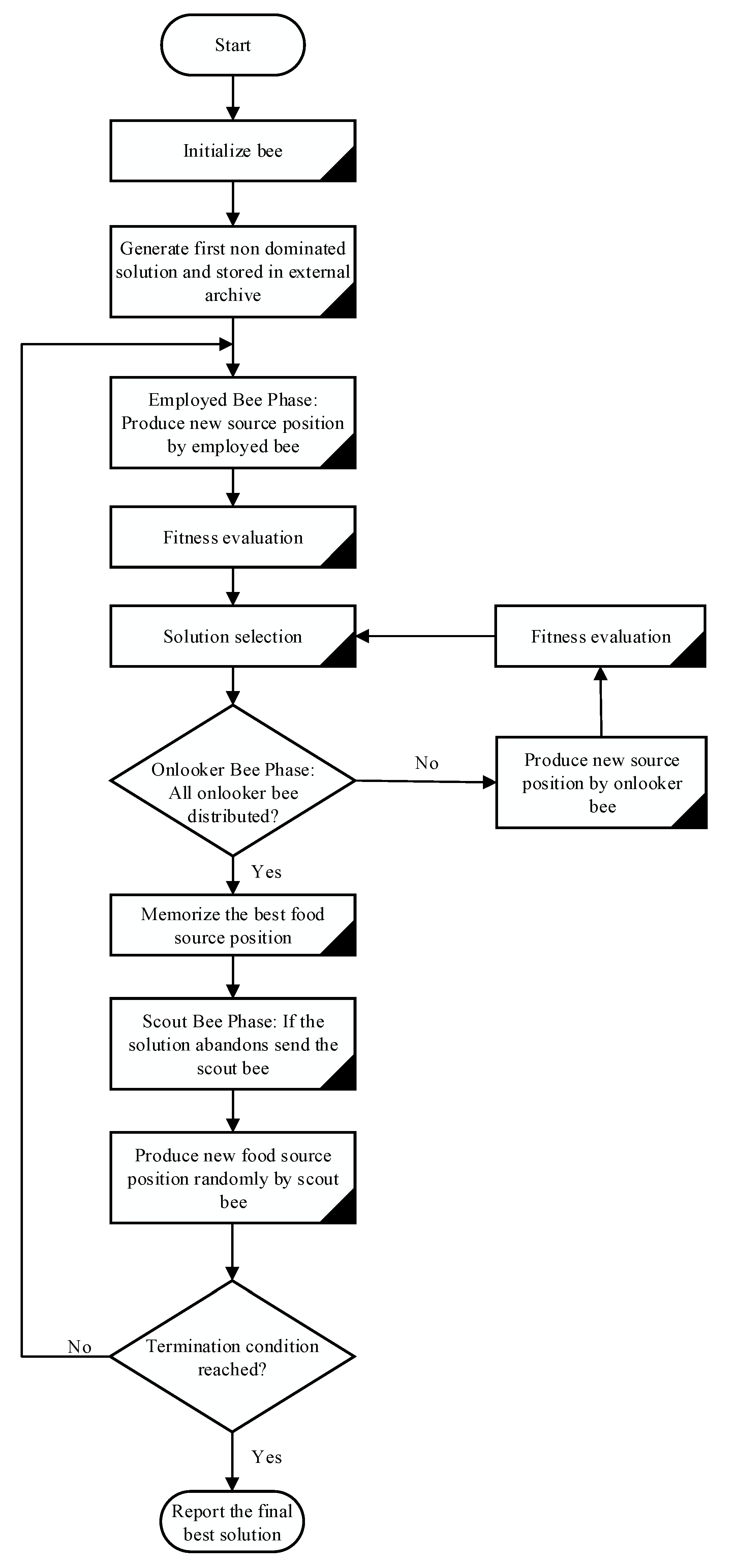
  • The Pareto approach and the external archive are integrated into the proposed MOABC algorithm.
After performing all of these modifications, the critical steps of the proposed MOABC algorithm are as follows:
  • Initialization phase
    • Initialize the food source position.
    • Define trail counter limit for the population and scout bees.
    • Generate the first non-dominated solution.
    • Generate external archives by inserting non-dominated solutions.
    • Define trial counters for the food sources.
    • Assign the food sources to the employed bees.
  • Employed bee phase
    • Produce a new position of the food source.
    • Evaluate the fitness of the identified food source position.
    • If the fitness of the new position is better than the old one, update the new position, and decrease the trial counter by 1; otherwise, increase it by 1.
  • Onlooker bee phase
    • Choose the solution from the population using tournament selection probability.
    • For each onlooker bee, produce a new food source position.
    • Evaluate the fitness of the candidate food source.
    • Apply the greedy selection procedure to choose the best source.
    • Save the best solution obtained so far.
  • Scout bee phase
    • If the solution cannot be improved after a limited number of trials, then a scout bee occurs, and a new food source position is produced.
    • Evaluate the fitness of the produced food-source position.
    • Reset its trial counter.
If a termination condition is reached, then report the final best solution else go to the employed bee phase.
The flowchart of the proposed MOABC algorithm is shown in Figure 4.

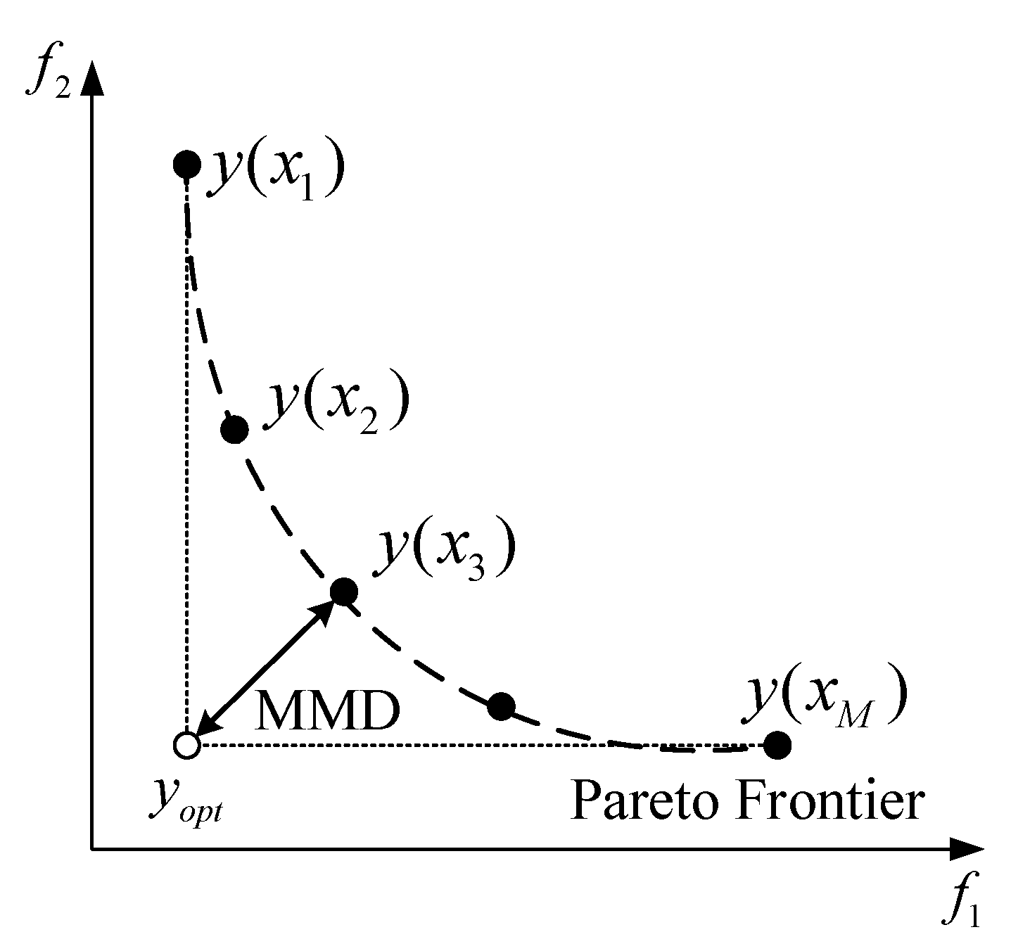
4.2.4. Multi-Criteria Decision Making

The selection of a final solution among the Pareto-optimal set is regarded as multiple criteria decision making (MCDM) in multi-objective optimization problems. In this study, a minimum Manhattan distance (MMD) method was used to select an appropriate solution from the non-dominated solutions to verify the superiority of the proposed MOABC method.
The Manhattan distance is the sum of the absolute differences in Cartesian coordinates for the distance between two points. The solution that minimizes the distance from the normalized ideal vector is the MMD, as depicted in Figure 5.
After normalization, the ideal vector y o p t is denoted as,
y o p t = [ 1 L 1 2 L 2 n L n ] t ,
1 = min x N y n ( x )       N = { x 1 ,   x 2 ,   ,   x M } ,
L n = max x N y n ( x ) min x N y n ( x ) .
In the set of all feasible solutions, the minimum distance sum between the ideal vector y o p t and the selected solution is defined as the MMD:
min x N | | y n ( x ) y o p t | | = min x N n = 1 M | | y n ( x ) L n n L n | | .

5. Simulation Result

5.1. Sample System

A system of 11.4 kV, 60 Hz, which included a harmonic source, was used for the simulation experiment to prove the efficiency and accuracy of the proposed method. The system with harmonic loads and various PPFs is shown in the line diagram depicted in Figure 6, where the nonlinear load is considered as the source of harmonic current, and the PPFs and the system can be regarded as the equivalent impedance. The remaining linear loads can be ignored, owing to the large impedance. In this study, three cases considered the harmonic filter planning. The system network was assumed to be balanced and the harmonic current, harmonic voltage without filters, and utility tolerance for all three cases are listed in Table 2, and it is evident that the fifth order harmonic current and current THD of Case 1 exceeded the tolerance value. In Case 2, the second order and fifth order harmonic current, fifth order harmonic voltage, current THD, and voltage THD all exceeded the tolerances. Moreover, the fifth order harmonic current and the fifth, seventeenth, and nineteenth harmonic voltages of Case 3 also exceeded the tolerances.

5.2. Setting Parameters

Therefore, the upper limit of the number of filters is set to three, and the passive filter design is performed with the investment cost set to an unlimited amount. The fundamental active power (load demand) of Case 1 was 14,590 kW, with a lagging pf of 0.892. For both Cases 2 and 3, a fundamental active power of 20 MW, with a lagging pf of 0.65 of fundamental active power was considered. The short-circuit current of the system was in the range of 8,268 to 19,695 A. The parameters of the MOABC and other optimization algorithms are listed in Table 3. The trial counter limit L was set to four. The general trial counter limit L of the original ABC algorithm [32] is related to the number of onlooker bees and the dimensions of the variables. However, the general trial counter limit L may decrease the number of scout bees in the scout-bee phase and discourage the exploration process.
The decision variables x ¯ i for the optimal design of PPFs include the resistance size, reactance size, and capacitor size. Therefore, vector x ¯ i can be defined as follows:
x ¯ i = [ L 1 ,   C 1 ,   R 2 ,   L 2 ,   C 2 , R 3 ,   L 3 ,   C 3 ] t .
The parameters of the proposed MOABC algorithm and the parameter ranges are listed in Table 4.

5.3. Accuracy Test

The generational distance (GD) was used to determine the accuracy of the proposed method. GD is a method introduced by Veldhuizen and Lamont [54] to check the closeness of any selected method to the true Pareto front. The true Pareto front optimal set is determined by the Monte Carlo method. GD can be defined as,
GD = m n d m 2 n ,
where d m represents the Euclidean distance between the solutions by the proposed method and the nearest member of the true Pareto optimal set, and n indicates the number of final solutions.
The closeness of the solution determined by any method with the solution of the true Pareto optimal set is inversely proportional to the GD value, that is, it lowers the value of the GD, to closer to the true Pareto front. If the GD is zero, all solutions are equal to the solutions of the true Pareto optimal set, which is an ideal case.
MOPSO was used for a comparison with the proposed MOABC. Both algorithms were executed 50 times with 500 iterations to verify the accuracy of the proposed method. It is evident from Table 5 that the GD results obtained by MOABC are better than those obtained by MOPSO. Figure 7 shows that the 100 non-dominated solutions are inserted in the external archive by MOABC in 42 iterations and 77 iterations are required using MOPSO. Therefore, MOABC can be considered faster than MOPSO.

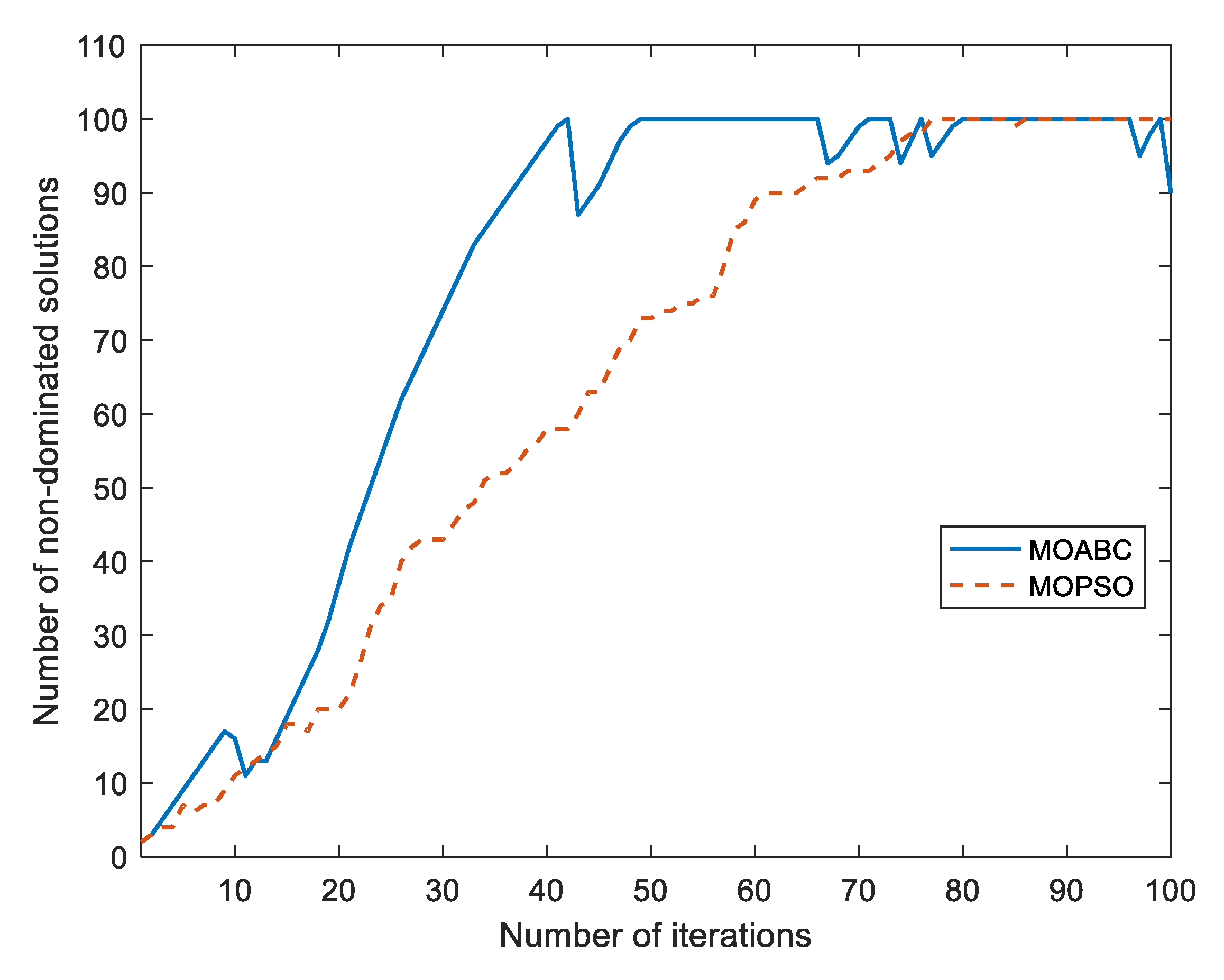
5.4. Performance Test

Regarding the performance of the proposed method, Table 6 lists the planning results of PPFs by MOABC compared to the results determined by the simulated algorithm (SA), which was introduced in [25] for all three cases, with a 0.95 lagging power factor in Case 1 and 0.97 lagging power factor in both Cases 2 and 3. The resistance (R), inductance (L), and capacitance (C) values are shown in ohm ( Ω ), m H , and μ F , respectively. The total cost, THDI, and THDV of PPF design by MOABC were lower than those determined by SA, and all the results were restrained under the tolerance limit of IEEE standard-519. As can be seen, the performance of the parameters obtained by the MOABC method is better than that of the SA method.
In Case 1, the fifth harmonic current and THDI exceeded the tolerance limit. Therefore, two single-tuned PPFs were used for elimination and to improve the reactive power. In Case 2, second order and fifth order harmonic had to be overcome. Therefore, a single-tuned PPF was used to mitigate the fifth order harmonic. However, the second order harmonic was enlarged. If another single-tuned is used to suppress the second order harmonic, then the system network faces overcompensation. Therefore, a C-type damped filter was used according to the topologies mentioned in Section 4. In Case 3, the fifth order harmonic current and seventeenth and nineteenth order harmonic voltages exceeded the limit tolerances of the IEEE standard. The single-tuned suppressed the fifth harmonic current, and a third order damped filter was used to eliminate the higher-order harmonic voltages for greater than the seventeenth order, but it enlarged the lower-order harmonics. In this situation, a C-type damped order was used to mitigate the second, third and fourth order harmonic currents. A second order damped filter can also be used instead of a third order damped filter.
For the MMD results, three cases were examined under four different PPF topologies. Table 7, Table 8 and Table 9 demonstrate the MMD results of MOABC with two other algorithms: MOPSO and MOBA for Cases 1, 2, and 3, respectively. In each case, 100 solutions obtained by each algorithm were merged, and then the most balanced solution was determined out of 300 solutions by MMD. The sequence of solutions is as follows: 1–100 (MOABC), 100–200 (MOPSO), and 200–300 (MOBA). Here, Type ‘1’, ‘2’, ‘3’, and ‘4’ denote single tuned PPF, second-order damped PPF, third-order damped PPF, and C-type damped PPF, respectively. In each case, the sequence of the most balanced solutions obtained by the MMD was between 1–100, representing the set of solutions obtained by MOABC. It can be seen that the performance of MOABC is better than that of MOPSO and MOBA in terms of the MMD results.

6. Conclusions

In this study, a new MOABC method was proposed to optimize the planning of PPF design. Four types of PPFs were considered in the optimization problem. Here, the objective functions of minimizing the total harmonic distortion of current and voltage, total cost, and of improving the power factor were used. In terms of accuracy, GD was used to evaluate the accuracy of the results obtained by MOABC and to compare the results with those obtained by MOPSO. The results indicate that the proposed method is highly accurate. In terms of performance, MOABC was compared with SA in three different cases. In each case, the results proved the superior performance of MOABC. In addition, the MMD obtained by MOABC was compared with the other two well-known metaheuristic algorithms (MOBA and MOPSO) for three different cases with four different PPF topologies in each. All the results obtained for MOABC were better than those of the algorithms mentioned above. Overall, a series of case studies and results have demonstrated the accuracy, superiority, and better performance of the proposed method, and present the potential to form PPF designs more efficiently.

Author Contributions

Conceptualization, N.-C.Y.; Data curation, N.-C.Y.; Funding acquisition, N.-C.Y.; Investigation, N.-C.Y., D.M. and K.-Y.L.; Methodology, N.-C.Y., D.M. and K.-Y.L.; Resources, N.-C.Y.; Software, N.-C.Y., D.M. and K.-Y.L.; Supervision, N.-C.Y.; Validation, N.-C.Y., D.M. and K.-Y.L.; Writing–original draft, N.-C.Y. and D.M.; Writing–review & editing, N.-C.Y. All authors have read and agreed to the published version of the manuscript.

Funding

This work was partially supported by the Ministry of Science and Technology (MOST) in Taiwan (MOST 109-3111-8-011-001) and Delta–NTUST Joint Research Center.

Institutional Review Board Statement

Not applicable.

Informed Consent Statement

Not applicable.

Data Availability Statement

Not applicable.

Conflicts of Interest

The authors declare no conflict of interest.

References

  1. Eroğlu, H.; Cuce, E.; Cuce, P.M.; Gul, F.; Iskenderoğlu, A. Harmonic problems in renewable and sustainable energy systems: A comprehensive review. Sustain. Energy Technol. Assess. 2021, 48, 101566. [Google Scholar] [CrossRef]
  2. Baliyan, A.; Jamil, M.; Rizwan, M. Power Quality Improvement Using Harmonic Passive Filter in Distribution System. In Advances in Energy Technology; Springer: Singapore, 2022; pp. 435–445. [Google Scholar]
  3. Michalec, L.; Jasiński, M.; Sikorski, T.; Leonowicz, Z.; Jasiński, L.; Suresh, V. Impact of Harmonic Currents of Nonlinear Loads on Power Quality of a Low Voltage Network–Review and Case Study. Energies 2021, 14, 3665. [Google Scholar] [CrossRef]
  4. Manito, A.; Bezerra, U.; Tostes, M.; Matos, E.; Carvalho, C.; Soares, T. Evaluating Harmonic Distortions on Grid Voltages Due to Multiple Nonlinear Loads Using Artificial Neural Networks. Energies 2018, 11, 3303. [Google Scholar] [CrossRef] [Green Version]
  5. Caicedo, J.; Romero, A.; Zini, H. Frequency domain modeling of nonlinear loads, considering harmonic interaction. In Proceedings of the 2017 IEEE Workshop on Power Electronics and Power Quality Applications (PEPQA), Bogota, Colombia, 31 May–2 June 2017; pp. 1–6. [Google Scholar]
  6. Gheisarnejad, M.; Mohammadi-Moghadam, H.; Boudjadar, J.; Khooban, M.H. Active power sharing and frequency recovery control in an islanded microgrid with nonlinear load and nondispatchable DG. IEEE Syst. J. 2019, 14, 1058–1068. [Google Scholar] [CrossRef]
  7. Ismael, S.M.; Aleem, S.H.A.; Abdelaziz, A.Y.; Zobaa, A.F. State-of-the-art of hosting capacity in modern power systems with distributed generation. Renew. Energy 2019, 130, 1002–1020. [Google Scholar] [CrossRef]
  8. Ali, Z.M.; Diaaeldin, I.M.; Aleem, S.H.E.A.; El-Rafei, A.; Abdelaziz, A.Y.; Jurado, F. Scenario-Based Network Reconfiguration and Renewable Energy Resources Integration in Large-Scale Distribution Systems Considering Parameters Uncertainty. Mathematics 2021, 9, 26. [Google Scholar] [CrossRef]
  9. Li, D.; Yang, K.; Zhu, Z.Q.; Qin, Y. A Novel Series Power Quality Controller with Reduced Passive Power Filter. IEEE Trans. Ind. Electron. 2016, 64, 773–784. [Google Scholar] [CrossRef]
  10. Azebaze Mboving, C.S. Investigation on the Work Efficiency of the LC Passive Harmonic Filter Chosen Topologies. Electronics 2021, 10, 896. [Google Scholar] [CrossRef]
  11. Bollen, M.H.; Das, R.; Djokic, S.; Ciufo, P.; Meyer, J.; Rönnberg, S.K.; Zavodam, F. Power Quality Concerns in Implementing Smart Distribution-Grid Applications. IEEE Trans. Smart Grid 2017, 8, 391–399. [Google Scholar] [CrossRef] [Green Version]
  12. Kalair, A.; Abas, N.; Saleem, Z.; Khan, N. Review of harmonic analysis, modeling and mitigation techniques. Renew. Sustain. Energy Rev. 2017, 78, 1152–1187. [Google Scholar] [CrossRef]
  13. Das, J.C. Passive filters—Potentialities and limitations. IEEE Trans. Ind. Appl. 2004, 40, 232–241. [Google Scholar] [CrossRef]
  14. Ahmed, M.; Nahid-Al-Masood; Aziz, T. An approach of incorporating harmonic mitigation units in an industrial distribution network with renewable penetration. Energy Rep. 2021, 7, 6273–6291. [Google Scholar] [CrossRef]
  15. Murugan, A.S.S. Meta-Heuristic Firefly Algorithm Based Optimal Design of Passive Harmonic Filter for Harmonic Mitigation. Int. Res. J. Adv. Sci. Hub 2021, 3, 18–22. [Google Scholar]
  16. Chang, G.W.; Wang, H.L.; Chuang, G.S.; Chu, S.Y. Passive Harmonic Filter Planning in a Power System with Considering Probabilistic Constraints. IEEE Trans. Power Deliv. 2009, 24, 208–218. [Google Scholar] [CrossRef]
  17. He, N.; Xu, D.G.; Huang, L.N. The Application of Particle Swarm Optimization to Passive and Hybrid Active Power Filter Design. IEEE Trans. Ind. Electron. 2009, 56, 2841–2851. [Google Scholar] [CrossRef]
  18. Chang, Y.P.; Tseng, W.K.; Tsao, T.F. Application of combined feasible-direction method and genetic algorithm to optimal planning of harmonic filters considering uncertainty conditions. IEE Proc.-Gener. Transm. Distrib. 2005, 152, 729–736. [Google Scholar] [CrossRef]
  19. Ko, C.N.; Chang, Y.P.; Wu, C.J. A PSO Method With Nonlinear Time-Varying Evolution for Optimal Design of Harmonic Filters. EEE Trans. Power Syst. 2009, 24, 437–444. [Google Scholar] [CrossRef]
  20. Kawann, C.; Emanuel, A.E. Passive shunt harmonic filters for low and medium voltage: A cost comparison study. IEEE Trans. Power Syst. 1996, 11, 1825–1831. [Google Scholar] [CrossRef]
  21. Lin, K.P.; Lin, M.H.; Lin, T.P. An advanced computer code for single-tuned harmonic filter design. IEEE Trans. Ind. Appl. 1998, 34, 640–648. [Google Scholar] [CrossRef]
  22. Makram, E.B.; Subramaniam, E.V.; Girgis, A.A.; Catoe, R. Harmonic Filter Design Using Actual Recorded Data. IEEE Trans. Ind. Appl. 1993, 29, 1176–1183. [Google Scholar] [CrossRef]
  23. Chen, Y.M. Passive filter design using genetic algorithms. IEEE Trans. Ind. Electron. 2003, 50, 202–207. [Google Scholar] [CrossRef]
  24. Chang, G.W.; Wang, H.L.; Chu, S.Y. Strategic placement and sizing of passive filters in a power system for controlling voltage distortion. IEEE Trans. Power Deliv. 2004, 19, 1204–1211. [Google Scholar] [CrossRef]
  25. Chou, C.J.; Liu, C.W.; Lee, J.Y.; Lee, K.D. Optimal planning of large passive-harmonic-filters set at high voltage level. EEE Trans. Power Syst. 2000, 15, 433–441. [Google Scholar] [CrossRef] [Green Version]
  26. Badugu, R.; Acharya, D.; Das, D.K.; Prakash, M. Class Topper Optimization Algorithm based Optimum Passive Power Filter Design for Power System. In Proceedings of the 2021 5th International Conference on Computing Methodologies and Communication (ICCMC), Erode, India, 8–10 April 2021; pp. 648–652. [Google Scholar]
  27. Wang, Y.; Liu, H.; Yin, K.; Yuan, Y. A Full-Tuned Filtering Method for Dynamic Tuning Passive Filter Power Electronics. J. Control. Autom. Electr. Syst. 2021, 32, 1771–1781. [Google Scholar] [CrossRef]
  28. Wang, Y.; Yin, K.; Liu, H.; Yuan, Y. A Method for Designing and Optimizing the Electrical Parameters of Dynamic Tuning Passive Filter. Symmetry 2021, 13, 1115. [Google Scholar] [CrossRef]
  29. Azab, M. Multi-objective design approach of passive filters for single-phase distributed energy grid integration systems using particle swarm optimization. Energy Rep. 2020, 6, 157–172. [Google Scholar] [CrossRef]
  30. Wang, S.; Ding, X.; Wang, J. Multi-objective optimization design of passive filter based on particle swarm optimization. J. Physics Conf. Ser. 2020, 1549, 032017. [Google Scholar] [CrossRef]
  31. Yang, N.-C.; Liu, S.-W. Multi-Objective Teaching–Learning-Based Optimization with Pareto Front for Optimal Design of Passive Power Filters. Energies 2021, 14, 6408. [Google Scholar] [CrossRef]
  32. Karaboga, D. An Idea Based on Honey Bee Swarm for Numerical Optimization; Technical Report-TR06; Erciyes University: Kayseri, Turkey, 2005. [Google Scholar]
  33. Karaboga, D.; Basturk, B. On the performance of artificial bee colony (ABC) algorithm. Appl. Soft Comput. 2008, 8, 687–697. [Google Scholar] [CrossRef]
  34. Mansouri, P.; Asady, B.; Gupta, N. The Bisection-Artificial Bee Colony algorithm to solve Fixed point problems. Appl. Soft Comput. 2015, 26, 143–148. [Google Scholar] [CrossRef]
  35. Benyoucef, A.S.; Chouder, A.; Kara, K.; Silvestre, S.; Sahed, O.A. Artificial bee colony based algorithm for maximum power point tracking (MPPT) for PV systems operating under partial shaded conditions. Appl. Soft Comput. 2015, 32, 38–48. [Google Scholar] [CrossRef] [Green Version]
  36. Zou, W.P.; Zhu, Y.L.; Chen, H.N.; Zhang, B.W. Solving Multiobjective Optimization Problems Using Artificial Bee Colony Algorithm. Discret. Dyn. Nat. Soc. 2011, 2011, 569784. [Google Scholar] [CrossRef] [Green Version]
  37. Karaboga, D.; Akay, B. A modified Artificial Bee Colony (ABC) algorithm for constrained optimization problems. Appl. Soft Comput. 2011, 11, 3021–3031. [Google Scholar] [CrossRef]
  38. Akay, B. Synchronous and asynchronous Pareto-based multi-objective Artificial Bee Colony algorithms. J. Glob. Optim. 2013, 57, 415–445. [Google Scholar] [CrossRef]
  39. Xiang, Y.; Zhou, Y.R. A dynamic multi-colony artificial bee colony algorithm for multi-objective optimization. Appl. Soft Comput. 2015, 35, 766–785. [Google Scholar] [CrossRef]
  40. Akbari, R.; Hedayatzadeh, R.; Ziarati, K.; Hassanizadeh, B. A multi-objective artificial bee colony algorithm. Swarm Evol. Comput. 2012, 2, 39–52. [Google Scholar] [CrossRef]
  41. Xiang, Y.; Zhou, Y.R.; Liu, H.L. An elitism based multi-objective artificial bee colony algorithm. Eur. J. Oper. Res. 2015, 245, 168–193. [Google Scholar] [CrossRef]
  42. Chu, R.F.; Wang, J.C.; Chiang, H.D. Strategic-Planning of Lc Compensators in Nonsinusoidal Distribution-Systems. EEE Trans. Power Deliv. 1994, 9, 1558–1563. [Google Scholar] [CrossRef]
  43. Deb, K.; Pratap, A.; Agarwal, S.; Meyarivan, T. A fast and elitist multiobjective genetic algorithm: NSGA-II. IEEE Trans. Evol. Comput. 2002, 6, 182–197. [Google Scholar] [CrossRef] [Green Version]
  44. Knowles, J.D.; Corne, D.W. Approximating the Nondominated Front Using the Pareto Archived Evolution Strategy. Evol. Comput. 2000, 8, 149–172. [Google Scholar] [CrossRef] [PubMed]
  45. Knowles, J.; Corne, D. Properties of an adaptive archiving algorithm for storing nondominated vectors. IEEE Trans. Evol. Comput. 2003, 7, 100–116. [Google Scholar] [CrossRef]
  46. Reyes-Sierra, M.; Coello, C.C. Multi-objective particle swarm optimizers: A survey of the state-of-the-art. Int. J. Comput. Intell. Res. 2006, 2, 287–308. [Google Scholar]
  47. Coello, C.C.; Lechuga, M.S. MOPSO: A proposal for multiple objective particle swarm optimization. In Proceedings of the 2002 Congress on Evolutionary Computation, Honolulu, HI, USA, 12–17 May 2002; pp. 1051–1056. [Google Scholar]
  48. Coello, C.A.C.; Pulido, G.T.; Lechuga, M.S. Handling multiple objectives with particle swarm optimization. IEEE Trans. Evol. Comput. 2004, 8, 256–279. [Google Scholar] [CrossRef]
  49. Chiu, W.-Y.; Yen, G.G.; Juan, T.-K. Minimum manhattan distance approach to multiple criteria decision making in multiobjective optimization problems. IEEE Trans. Evol. Comput. 2016, 20, 972–985. [Google Scholar] [CrossRef] [Green Version]
  50. Mernik, M.; Liu, S.H.; Karaboga, D.; Crepinsek, M. On clarifying misconceptions when comparing variants of the Artificial Bee Colony Algorithm by offering a new implementation. Inf. Sci. 2015, 291, 115–127. [Google Scholar] [CrossRef]
  51. Xiang, Y.; Peng, Y.M.; Zhong, Y.B.; Chen, Z.Y.; Lu, X.W.; Zhong, X.J. A particle swarm inspired multi-elitist artificial bee colony algorithm for real-parameter optimization. Comput. Optim. Appl. 2014, 57, 493–516. [Google Scholar] [CrossRef]
  52. Yang, N.C.; Le, M.D. Multi-objective bat algorithm with time-varying inertia weights for optimal design of passive power filters set. IET Gener. Transm. Distrib. 2015, 9, 644–654. [Google Scholar] [CrossRef]
  53. IEEE Recommended Practices and Requirements for Harmonic Control in Electrical Power Systems; IEEE: New York, NY, USA, 1993; pp. 1–100.
  54. Van Veldhuizen, D.A.; Lamont, G.B. Multiobjective Evolutionary Algorithm Research: A History and Analysis. 1998. Available online: http://citeseerx.ist.psu.edu/viewdoc/summary?doi=10.1.1.35.8924 (accessed on 1 October 2021).
Figure 1. Types of passive power filters: (a) single-tuned filter, (b) second-order damped filter, (c) third-order damped filter, and (d) C-type damped filter.
Mathematics 09 03187 g001
Figure 2. Harmonic circuit of a simple system with a nonlinear load and a set of passive power filters (a) one-line diagram and (b) equivalent harmonic circuit model.
Mathematics 09 03187 g002
Figure 3. Graphical representation of inserting a new non-dominated solution when the external archive is full.
Mathematics 09 03187 g003
Figure 4. Flowchart of the proposed MOABC algorithm.
Mathematics 09 03187 g004
Figure 5. Interpretation of the MMD.
Mathematics 09 03187 g005
Figure 6. Schematic diagram of a system with PPFs and nonlinear loads.
Mathematics 09 03187 g006
Figure 7. Number of non-dominated solutions inserted into the external archive of MOABC and MOPSO.
Mathematics 09 03187 g007
Table 1. Harmonic impedance of PPFs.
Type R F ( h )   X F ( h )  
ST R hX L X C h
SD R ( hX L ) 2 R 2 + ( hX L ) 2 R 2 hX L R 2 + ( hX L ) 2 X C h
TD 1 R ( hX L ) 2 R 2 + ( hX L X C h ) 2 R 2 hX L h X L 2 X C + X L X C 2 h R 2 + ( hX L X C h ) 2 X C h
CD 2 R ( hX L X L h ) 2 R 2 + ( hX L X L h ) 2 R 2 ( hX L X L h ) R 2 + ( hX L X L h ) 2 X C h
1 In TD PPFs, X C = 1 / ( ω C 2 ) ,   C 1 = C 2 . 2 In CD PPFs, X C = 1 / ( ω C 2 ) ,   C 1 = 1 / ( ω 1 2 L ) .
Table 2. Distributions of harmonic current and voltage without passive power filters.
CasesHarmonic OrdersCurrent, AVoltage, VIEEE Standard 519
Current, ACurrent, %Voltage, VVoltage, %
Case 11828.376581.79----
27.0211.188.281197.53
38.6420.6333.14197.53
45.9218.858.281197.53
545.8182.333.14197.53
719.0105.933.14197.53
1115.4134.916.62197.53
139.497.2816.62197.53
THD (%)6.554.11-5-5
Case 211558.36581.79----
219.230.5715.581197.53
336.887.8862.334197.53
45.4117.2315.581197.53
598.0390.162.334197.53
718.0100.362.334197.53
1113.2124.331.172197.53
1312.6130.431.172197.53
THD (%)7.046.86-5-5
Case 311558.36581.79----
29.4515.0515.581197.53
315.637.2662.334197.53
43.7712.015.581197.53
562.7249.662.334197.53
721.0117.062.334197.53
1119.4166.931.172197.53
1317.0175.931.172197.53
1716.0216.523.381.5197.53
1915.5234.423.381.5197.53
THD (%)4.927.42-5-5
Table 3. Parameters of MOABC and other optimization algorithms.
ParameterMOABCMOPSOMOBA
Number of iterations200200200
Population size202020
Other related parametersTrial counter limit,
L = 4
Number of employed bees,
Employzise = 20
Number of onlookers,
Onlookersize = 20
Number of scouts,
Scoutsize = 20
Cognitive parameter,
c 1 = 2.0
Social parameter,
c 2 = 2.0
Maximum frequency,
F m a x = 2.0
Minimum frequency,
F m i n = 2.0
Constants,
α = 0.9 γ = 0.9
Table 4. Parameters of the proposed MOABC algorithm.
ItemFeasible Ranges of Parameters
Number of iterations 200
Population size20
Number of objectives4
Number of constraints22
Size of external archive100
Number of divisions30
Maximum initial IC4000 pu
R for PPFs0.01–100 Ω
L for PPFs0.01–50 mH
C for PPFs0.01–900 μF
Table 5. Generational distance determined by MOABC and MOPSO (50 running times- 500 iterations).
TitleGenerational Distance
BestWorstAverageMedianStd. Dev
MOABC0.000001230.01860.00016460.00011930.000499
MOPSO0.000001960.02580.00024590.00017070.000854
Table 6. Comparisons of passive-filter design results of MOABC with SA.
CasesTypes of FiltersMOABCSA
Case 1
(PF = 0.95)
Single-tuned ( F 1 ) L 1 = 13.75 L 1 = 15.37
C 1 = 22.67 C 1 = 20.27
Single-tuned ( F 2 ) L 2 = 17.64 L 2   = 16.45
C 2   = 27.62 C 2 = 29.61
THD I   (%)4.704.79
THD V   (%)1.291.30
Cost (pu)233.70234.26
Case 2
(PF = 0.97)
Single-tuned ( F 1 ) L 1 = 3.86 L 1   = 4.32
C 1   = 80.86 C 1 = 72.24
C-Type ( F 2 ) R 2 = 54.18 R 2 = 51.84
L 2 = 8.72 L 2 = 8.21
C 2 = 295.79 C 2 = 302.40
C * = 806.90 C * = 857.03
THD I   (%)4.934.95
THD V   (%)1.321.35
Cost (pu)3176.233280.66
Case 3
(PF = 0.97)
Single-tuned ( F 1 ) L 1 = 3.12 L 1 = 3.67
C 1 = 100.00 C 1 = 105.42
3rd-order ( F 2 ) R 2 = 18.46 R 2 = 15.37
L 2 = 6.76 L 2 = 4.30
C 2 = 54.95 C 2 = 35.68
C-Type ( F 3 ) R 3 = 24.5 R 3 = 40.44
L 3 = 39.40 L 3   = 15.25
C 3 = 209.05 C 3 = 218.95
C * = 178.58 C * = 461.39
THD I   (%)3.874.81
THD V   (%)1.892.11
Cost (pu)1827.382431.17
In CD PPFs,   C * = 1 / ( ω 1 2 L ) .
Table 7. MMD result by merging all the three algorithms: MOABC (1–100), MOPSO (101–200), and MOBA (201–300) for Case 1.
Type of FiltersSol. No.ParameterCostTHDITHDVPF
L 1 C 1 R 2 L 2 C 2 C * R 3 L 3 C 3 C *
1074.1396.13 204.654.851.210.99
1354.5468.70 311.243.761.040.99
1 16.9528.75
1677.0744.13 496.854.231.130.99
2 51.2010.4650.00
1768.0138.95 665.614.411.180.98
3 48.3712.3647.70
Table 8. MMD result by merging all the three algorithms: MOABC (1–100), MOPSO (101–200), and MOBA (201–300) for Case 2.
Type of FiltersSol. No.ParameterCostTHDITHDVPF
L 1 C 1 R 2 L 2 C 2 C * R 3 L 3 C 3 C *
1333.4590.35 3461.574.801.260.98
4 51.317.71310.27912.61
1112.76113.11 3651.034.851.190.99
1 24.3620.00
4 84.758.32277.42845.70
1483.5188.76 3917.314.761.260.99
2 86.7734.2734.49
4 87.858.85273.56795.05
1013.5787.28 3983.804.581.230.99
3 99.9116.8653.82
4 81.599.76260.48720.92
Table 9. MMD result by merging all the three algorithms: MOABC (1–100), MOPSO (101–200), and MOBA (201–300) for Case 3.
Type of FiltersSol. No.ParameterCostTHDITHDVPF
L 1 C 1 R 2 L 2 C 2 C * R 3 L 3 C 3 C *
1463.2396.51 913.743.631.840.99
1 10.4046.88
2 22.2010.02189.74
1583.12100.00 1345.243.831.880.99
1 8.6956.05
3 28.8219.80142.50
1213.9778.48 2078.883.841.410.98
2 100.01.4642.69
4 24.1450.00274.03140.72
1664.8564.31 1874.343.991.630.99
3 25.212.1459.11
4 12.3747.55286.64147.97
Publisher’s Note: MDPI stays neutral with regard to jurisdictional claims in published maps and institutional affiliations.

