A Mixed Statistical and Machine Learning Approach for the Analysis of Multimodal Trail Making Test Data

Abstract

Eye-tracking can offer a novel clinical practice and a non-invasive tool to detect neuropathological syndromes. In this paper, we show some analysis on data obtained from the visual sequential search test. Indeed, such a test can be used to evaluate the capacity of looking at objects in a specific order, and its successful execution requires the optimization of the perceptual resources of foveal and extrafoveal vision. The main objective of this work is to detect if some patterns can be found within the data, to discern among people with chronic pain, extrapyramidal patients and healthy controls. We employed statistical tests to evaluate differences among groups, considering three novel indicators: blinking rate, average blinking duration and maximum pupil size variation. Additionally, to divide the three patient groups based on scan-path images—which appear very noisy and all similar to each other—we applied deep learning techniques to embed them into a larger transformed space. We then applied a clustering approach to correctly detect and classify the three cohorts. Preliminary experiments show promising results.

1. Introduction and Related Work

Eye-tracking offers a fundamental tool to process and analyse human brain behaviour by detecting eye position and speed of movements [1]. Moreover, eye movements could in principle be used in order to highlight the presence of pathological states, and consistent research has been recently performed in this direction [2,3]. In the last decades, Machine Learning (ML) has been widely applied to many different research fields [4,5,6,7] and, in particular, some examples of its use for Trail Making Test (TMT) data analysis can be found in the literature. For instance, in [8], an approach based on random forests, decision trees and Long Short Term Memories (LSTMs) was proposed to detect the presence of a pathological state in the tested subjects. In particular, 60 patients were recruited in the study, 24 of which presenting brain injury and 36 presenting vertigo episodes. Similarly, in [9], the eye-tracking test was used to analyse children diagnosed with autism spectrum disorder (ASD), in order to establish a quantitative relationship between their gaze performance and their ability in social communication. Indeed, in the same study, the eye gaze-tracking was proposed as a possible non-invasive, quantitative biomarker to be used in children with ASD. Finally, a vast literature exists related to applications of eye-tracking tests to detect depression syndromes [10,11,12,13], and eye-tracking studies have proved their efficacy in the diagnosis of other common neurological pathologies, such as Parkinson’s disease, brain trauma and neglect phenomena [14,15,16,17], while ML techniques have been recently applied to process TMT data for the detection of the Alzheimer’s disease [18,19].

In [20], a new experiment based on TMT has been proposed, called the Visual Sequential Search Test (VSST). In a standard TMT experiment, a subject is presented with a sheet of numbers and letters arranged in a random manner and is asked, using a pen, to perform two tasks simultaneously, namely, to connect both in progressive and alternating order numbers and letters. In the VSST setting, the patients are required to carry on the same task based only on eye movements. Human visual search [20,21] is, in fact, a common activity that enables humans to explore the external environment to take everyday life decisions. Indeed, sequential visual search should use a peripheral spatial scene classification technique to put the next target in the sequence in the correct order, a strategy which, as a byproduct, could also improve the discriminatory ability of human peripheral vision and save neural resources associated with foveation. With respect to the cohorts of patients under examination, data were collected from people with chronic pain, extrapyramidal patients and healthy controls. In particular, individuals affected by extrapyramidal symptoms suffer from tremors, rigidity, spasms, decline in cognitive functions (dementia), affective disorders, depression, amnesia, involuntary and hyperkinetic jerky movements, slowing of voluntary movements such as walking (bradykinesia), and postural abnormalities. Conversely, there are several mechanisms underlying chronic pain; more often an excessive and persistent stimulation of the “nociceptors” or a lesion of the peripheral or central nervous system, but there are also forms of chronic pain that do not seem to have a real, well-identified cause (neuropathic pain). Therefore, chronic pain can be related to a variety of diseases, with very different severity, from depression, to chronic migraine and to cancer.

In [22], an algorithmic approach for the analysis of the VSST, based on the episode matching method, is proposed. In this paper, instead, we analyse the VSST data from a different perspective, examining both the blinking behaviour and the pupil size of the subjects and the freezed images of the scan-paths captured during the test, to gain an insight into the patient condition and offer a support for the clinical practice. For this purpose, we have compared several indicators to distinguish among classes of patients. A first preliminary analysis was performed, to evidence statistical differences based on pupil-derived measures. Such analysis showed the presence of statistically diversified behaviours existing among healthy, chronic and extrapyramidal subjects. Moreover, we further implemented a Deep Learning (DL) autoencoder architecture, with a U-Net backbone [23], to reconstruct the trajectory images for the three groups of individuals. Subsequently, as a proof of concept, we analysed the latent embedding representations using the K-means clustering algorithm, to verify the presence of clusters corresponding to the three cohorts of patients. Preliminary experiments actually evidence well-defined phenotypical groups in the latent space.

The paper is organised as follows. In Section 2, the VSST and the dataset used are described, together with the statistical methodologies and the DL approach employed for analysing pupils and image data. In Section 3, we summarise and discuss the obtained results. Finally, Section 4 collects some conclusions and traces future work perspectives.

2. Materials & Methods

2.1. Visual Sequential Search Test

The Trail Making Test is used in clinical practice as a neuropsychological assessment of visual attention and task switching. The test investigates the subject’s attentive abilities and the capability to quickly switch from a numerical to an alphabetical visual stimulus. Successful performance of the TMT requires a variety of mental abilities, including letter and number recognition, mental flexibility, visual scanning and motor function [24].

The research described in this paper used an oculomotor-based methodology, called eye-tracking, to study cognitive impairments in patients affected by chronic pain and extrapyramidal syndrome. Eye-tracking is in fact a promising way to carry out this kind of cognitive tests, allowing the recording of eye movements, to determine where a person is looking, what the person is looking at and for how long the gaze remains in a particular spot. More precisely, an eye-tracker uses invisible near-infrared light and high-definition cameras to project the light into the eye and record the direction in which it is reflected by the cornea [25]. Advanced algorithms are then used to calculate the position of the eye and determine exactly where it is in focus. This makes it possible to measure the visual behaviour and fine eye movements and allows for a more subtle exploration of cognitive dysfunction in a range of neurological disorders.

Several different eye-tracking devices exist, for example, the screen-based eye-tracker [26]. This type of test requires respondents to sit in front of a monitor and to interact with a screen-based content. In the experiments described in this paper, we made use of a special type of TMT experiment, namely the Visual Sequential Search Test. Such test has been created for studying the top-down visual search, which can be summarised as a series of saccades and fixations. In particular, the VSST consists of a repeated search task, and patients are asked to make the connection by looking at a logical sequence of numbers and letters. Here, the required task is to follow with the movement of the eyes the alphanumeric sequence 1-A, 2-B, 3-C, 4-D, 5-E, as shown in Figure 1.

2.2. VSST Experimental Dataset Description

Three types of individuals were recruited for the experiments. In particular: 46 patients with extrapyramidal syndrome, 284 affected by chronic pain and 46 controls. For each person, the eye-tracker provided the following information:

• average gaze position along x axis (pixels);
• average gaze position along y axis (pixels);
• fixation ID (integer) ($-1$ = saccade);
• pupil size (left);
• pupil size (right);
• timestamp (every 4 ms);
• stimulus (code of the image shown in the screen).

Regular eye movements alternate between saccades and visual fixations. A fixation consists in maintaining the visual gaze on a single location. A saccade, instead, is a quick, simultaneous movement of both eyes, between two or more phases of fixation in the same direction. In case of blinking, the device loses the signal, which results in $NaN$ value recorded in our dataset, either for the position $(x,y)$ on the screen and for the size of the pupils.

Data preprocessing was necessary before proceeding with the analysis. In particular, we deleted the experiment part not referring to the image labelled as “TMT stimulus” (Figure 1), we uniformed the timing to have timestamps exactly every 4 ms, and all the artefacts and noisy information were removed from the dataset (e.g., repeated rows).

2.3. ETT Image Dataset

To generate the 2D images of the gaze trajectories, the size of the left pupil and the average positions of the gaze along the horizontal and vertical axes were extracted from the preprocessed numerical data acquired by the eye-tracker during the experiments. In this context, pupil size values equal to $NaN$ correspond to the eye blinks and to those movements recorded while the eye was closed. Therefore these data were removed from the trajectories, as shown in Figure 2.

The ETT (Eye-Tracking Trajectory) dataset is composed of images of dimension 1920 × 1080 pixels, composed by a single colour channel. Binary images constituting the dataset consists of a black background (value 0) where the pixels corresponding to the gaze trajectory appear in white (value 255). In other words, each image is a binarised single-channel (greyscale) image, with intensity values belonging to $\{0,255\}$. No smoothing operation was performed on the trajectories, in order to preserve the original data information. ETT includes 376 images (46 healthy controls, 46 extrapyramidal patients and 284 chronic pain patients). To generate the dataset, we made use of MATLAB 2021a software [27].

2.4. Statistical and Deep Learning Methods for the VSST Data Analysis

In the following subsections, we describe how the two sources of information from the VSST can be processed. On the one hand, the behaviour of the population of our patients is analysed with statistical methods applied to the morphological characteristics of the pupil and to the blinking frequency. On the other hand, the images belonging to the ETT dataset were preprocessed on the basis of a DL method, to obtain a latent representation that allows us to adequately group the three cohorts of examined individuals.

2.4.1. Statistical Methods

The following markers were extracted for each patient: the difference between the maximum and the minimum value of the pupil size (averaged over the right and left eye), the blinking rate (i.e., the number of blinks per second) and the blinking average duration. For each of these continuous variables, its distribution over the three classes of patients was computed. Afterwards, a Kruskall–Wallis test [28] was performed. This nonparametric test is used for verifying whether samples originate from the same population (or from populations with equal median). The test has been extensively used for several statistical applications, and has been proved to be a very powerful alternative to parametric tests [29]. It can compare two or more independent samples of different size, testing the null hypothesis $H_0$, defined by

$$H_0:{\lambda }_1={\lambda }_2=\dots ={\lambda }_n,$$

where ${\lambda }_i$ is the median of the ith distribution sample.

In order to detect and remove the outliers of each distribution, we applied the unimodal Chebyshev Theorem, with $\gamma =3$ [30]. This resulted in keeping at least 89% of the values around the mean. Then, we repeated the statistical analysis with the cleaned samples. Finally, a bootstrapping method was performed to avoid the potential effect on the results, due to the difference between the sample size of the chronic pain patients compared to the size of the other two.

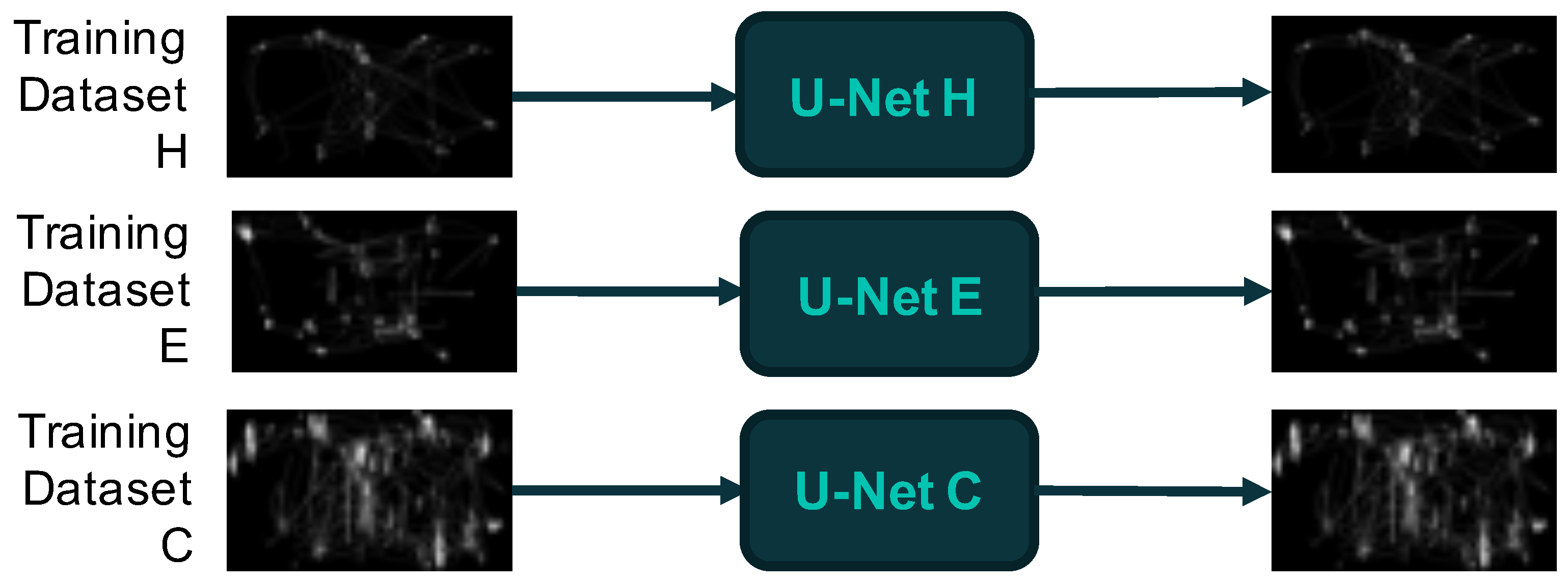
2.4.2. Deep Learning Modelling: Autoencoders and the U-Net Architecture

Deep learning has reached state of the art performance in image processing and analysis for a wide range of applications, in particular it gives excellent results in tasks such as image classification, detection or segmentation, see [31,32,33]. In the present work, we made use of a U-Net-based architecture, a DL model well known for its very good performance in image processing tasks [34]. This model was originally proposed as an efficient and fast way to perform biomedical image segmentation [34]. The architecture is composed by several convolutional layers, which take the original image as input and produce their segmentation maps. It is based on an encoder–decoder structure and can, therefore, be successfully used also to perform image reconstruction. As a matter of fact, in our paper, we trained the U-Net based architecture to reproduce the original image at the output, obtaining a network which is capable of reconstructing the input images (see Figure 3). The architecture used for the present work can thus be viewed as a deep learning, self-supervised autoencoder, made of a downsampling stage (encoder) and an upsampling stage (decoder). The overall scheme of the deep learning architecture proposed, is depicted in Figure 4.

In the encoder stage of the network, the spatial dimension is reduced by convolutional blocks followed by a maxpool downsampling layer, while the channel dimension is increased, to encode the input image into a hidden representation at multiple different levels, by means of a series of convolutional layers which use filters to get the so-called feature maps. A single feature map provides an insight into the internal representation for the specific input for each of the convolutional layers in the model, capturing some specific information from the input data, such as curves, straight lines or a combination of them. The decoder stage, instead, increases the latent spatial dimension while reducing the number of channels, using convolution blocks followed by an upsampling layer. Generally, the U-Net architecture implies a series of concatenation operations between the output of a layer of the encoder and the input of the corresponding layer in the decoder, by means of residual connections. As the model used acts as an autoencoder, the residual connections have been eliminated, so that the decoder can use only the output of the encoding stage, without including in the reconstruction phase the additional information given by this type of connections. This, also, allows us to avoid overfitting of the reconstruction network, given the small amount of images available. More specifically, 1024 feature maps, each of size 67 × 120 pixels, are obtained from a binarised image of shape 1920 × 1080 × 1, as shown in Figure 5. As a single feature map captures certain aspects from the input data, all the aforementioned 1024 feature maps have been therefore flattened and concatenated to obtain the image embedding representation of shape 1× 8,232,960. Some examples of intermediate representations obtained for a random image for each class are shown in Figure 6.

The model was developed in Python version 3.9.5 with Tensorflow 2.4.0 (Keras backend), and trained using Adam optimizer with an initial learning rate equal to ${10}^{-4}$. All the experiments were performed on a Linux–based machine equipped with an Intel Core i9-10920X CPU, 128 GB DDR4 RAM and a Titan RTX GPU with 24 GB GDDR6 VRAM.

2.4.3. K-Means Clustering

As a proof of concept, we performed clustering in both the original and latent space, obtained with our U-Net based model. This would in fact allows to show the ability of the image reconstruction architecture to efficiently compress and maintain the information contained in the original images, producing latent representations which are easier to be distinguished in the three different cohorts [35]. With this intent, we used the K-means [36] algorithm, one of the best known and most used partition clustering methods. The algorithm is based on an optimisation process whose aim is to minimise the intra-cluster variance. The number of clusters, K, needs to be specified in advance. On the first iteration, K clusters are created. Thereafter, the representatives for each cluster are calculated iteratively, until convergence. We used the Scikit-learn Python (Version 3.1).

The K-means algorithm has been applied to input data (belonging to the ETT dataset) as well as to the reconstructed data: all the examples in both settings have been grouped in a single cluster, except for only three examples—all belonging to the chronic pain patient category—which have been assigned to the other two clusters. A different strategy was then applied, based on the latent space representations and K-means, to determine if collecting the different feature maps, resulting from image compression, was able to lead to a correct grouping of the three categories of patients.

3. Results and Discussion

3.1. Statistical Analysis of Pupil and Blinking Data

First, the Kruskall–Wallis test was applied to the distributions of the blinking rate, maximum pupil size variations and mean blinking duration. In Figure 7, we show the distributions of the three indicators, for healthy, chronic and extrapyramidal individuals. Similarly, in Figure 8, we show boxplots for the three indicators, comparing the three groups.

We further performed the Kruskall–Wallis test, to compare the three groups’ distributions. The level of statistical significance chosen is p-value = 0.05.

As shown in

Table 1. Kruskal–Wallis test results of the pairwise comparison between Healthy (H), Chronic (C) and Extrapyramidal (E) subjects for blinking rate, maximum pupil size variation and blinking average duration. Significant p-values are highlighted in bold.

	Blinking Rate		Maximum Pupil Size Variation		Blinking Average Duration
Classes	p-Value	H Statistic	p-Value	H Statistic	p-Value	H Statistic
H–C	0.0059	7.5880	0.0121	6.2899	0.1079	2.5847
H–E	0.2092	1.5771	0.6534	0.2016	0.5289	0.3966
E–C	0.3258	0.9654	0.0039	8.3394	0.0058	7.6226

, no significant differences are found between healthy subjects and patients affected by extrapyramidal syndrome considering the three indicators. Conversely, a significant statistical difference between healthy controls and chronic pain patients was found for the rate of blinking and the variation of pupil size. Concerning the comparison between patients affected by chronic pain and extrapyramidal syndrome, a significant difference was detected both in the maximum pupil size variation and in the blinking average duration. In Table 1, also the H statistic value is reported, which represents the test statistic for the Kruskal–Wallis test. Under the null hypothesis, the $\chi$-square distribution approximates the distribution of H.

3.1.1. Outliers Detection and Kruskall–Wallis Test

A further step of the analysis, as described in Section 2.4.1, consisted in repeating the Kruskal–Wallis test on distributions without outliers. The Chebyshev outlier detection method uses the Chebyshev inequality to calculate the upper and lower outlier detection limits. Data values outside this range will be considered outliers. The outliers could be due to an incorrect acquisition procedure or they could indicate that the data are correct but highly unusual. The results of the Kruskall–Wallis test on the cleaned distributions are reported in

Table 2. Kruskal–Wallis test results of the pairwise comparison between Healthy (H), Chronic (C) and Extrapyramidal (E) subjects for blinking rate, maximum pupil size variation and blinking average duration. Significant p-values are highlighted in bold.

	Blinking Rate		Maximum Pupil Size Variation		Blinking Average Duration
Classes	p-Value	H Statistic	p-Value	H Statistic	p-Value	H Statistic
H–C	0.0027	9.0171	0.0075	7.1445	0.0488	3.8814
H–E	0.1877	1.7355	0.4984	0.4584	0.5115	0.4309
E–C	0.2390	1.3867	0.0008	11.3152	0.0016	9.999

.

The analysis based on clean samples confirmed the previous results: all the significant p-values remained such and, in general, they even decreased. As an effect of this reduction, the difference between Healthy and Chronic subjects in the blinking average duration became significant.

3.1.2. Bootstrapping Method

Although the Kruskal–Wallis test is designed for different sample size groups, the greater number of chronic patients than the other two classes may affect the results to some extent. To avoid this kind of bias, we performed the analysis described in the following. A sample of chronic patients was randomly selected from the original distribution, with a size equal to the others—46 patients, and then the Kruskal–Wallis test was applied. This resampling operation is repeated 10,000 times.

Table 3. Percentage of p-value below the threshold of significance equal to 0.05 for the Kruskal–Wallis test of the pairwise comparison of Healthy and Extrapyramidal patients with the resampled Chronic patients.

Classes	Blinking Rate	Maximum Pupil Size Variation	Blinking Average Duration
H–C	59.11%	48.06%	10.99%
E–C	2.05%	67.92%	58.42%

reports the percentage of p-values less than 0.05 over the 10,000 runs.

The bootstrapping procedure allows us to validate the results in Table 1. Indeed, only the comparison between Healthy and Chronic patients with respect to the variation of pupil size has a percentage of significant p-values less than 50% (in particular equal to 48.06%), while this indicator has shown to be significant in the previous experiments. Therefore, we can conclude that, based on the considered indicators, healthy and extrapyramidal subjects look indistinguishable, while chronic pain patients behave significantly different. This is not an astonishing result as neurophysiological studies [37] suggested that a painful electrical stimulation is associated with consistent alterations in the eye muscle activity. Moreover, altered results of the Blink Reflex (BR) test normally stand for a dysfunction in brain stem and trigeminovascular connections of patients with migraine headache, supporting the trigeminovascular theory of migraine [38].

3.2. Mapping Latent Space Representations of ETT Images to Phenotypic Groups

For what concerns the analysis of the ETT dataset, three U–Net based autoencoders—one for each group, all sharing the same architecture and the same set of initial random weights—were trained for image reconstruction. In particular, the generic U–Net${}_i$ is trained only on the data describing the ith class of individuals, which means that the U–Net${}_H$ has been trained to reconstruct input images from the healthy class only, while U–Net${}_E$ and U–Net${}_C$ are trained on extrapyramidal and chronic classes, respectively. The workflow of the analysis is depicted in Figure 9.

The experiments were carried out as described in the following. The three U-Net architectures were originally trained on 46 healthy, 46 extrapyramidal and 284 chronic pain patients, respectively, i.e., with the entire ETT dataset. Moreover, to obtain a balanced training set, experiments were also performed with only 46 chronic pain randomly sampled patients. The three encoder outputs were concatenated in a unique matrix, whose “entries” (latent representations of ETT images) were then clustered using the K-means algorithm, with $K=3$.

The pipeline of the procedure is depicted in Figure 10. The number of clusters is empirically defined by the structure of the dataset itself, as it contains three types of individuals known a priori. The K-means algorithm is not used for classification purposes, but with the intent of evaluating the presence of usueful information in the latent embeddings which allows to properly discern the three groups. In each of the three groups, only subjects belonging to the same cohort are present, showing the possibility of properly dividing patients into groups using the latent space embeddings.

Considering such preliminary results, we decided to implement a procedure to test the generalisation capability of the models. Therefore, we trained the three U-Nets only on 41 samples for each class of individuals. The test set, consisting of five healthy, five chronic and five extrapyramidal samples, was used as input to the three architectures separately. Subsequently, we ran the K-means algorithm ($K=3$) with respect to the matrix obtained as the mean values along the embedding dimension of the test embeddings obtained at the previously described step. Next, we clustered the new mean values matrix, checking if the three clusters detected correspond to the three groups. In particular, the mean healthy embeddings obtained with the three architectures ended up in the same cluster, with 67% of accuracy. On the other hand, there was no remarkable distinction for the chronic and extrapyramidal patients. Moreover, as a further proof of concepts, we averaged the embedding representations, for each group of individuals and for each model—obtaining the vectors of the mean values for the reconstructed embeddings and clustering the corresponding matrix with K-means ($K=3$) to verify whether the three averaged embeddings for the generic class could give an insight of the relationship between the input image class (healthy, chronic and extrapyramidal) in the embedding space. All of the three resulting mean “Healthy” reconstructed vectors of embeddings were clustered in the same community. Instead extrapyramidal and chronic patients, were not distinctively divided in their respective groups. This shows a similar behaviour to what we detected with the testing procedure. Healthy individuals trajectories are, in fact, more characterisable comparing to the two other subject categories.

Nonetheless, classifying the three groups of individuals based on DL techniques applied to ETT images remains a very difficult task, especially because of the scarcity of data and due to the complexity of the task itself. Indeed, human experts are unable to recognise different types of patients looking at the “frozen” trajectories they follow to approach the VSST, both because such trajectories are not so different to the naked eye and because, in the freezing process, the important temporal information on the way in which each trajectory is travelled, is irremediably lost. Taking into account, with an ad hoc preprocessing, of the sequential nature of the data and, most of all, enlarging the training dataset will surely allow better results.

4. Conclusions

In this paper, we presented some preliminary results on the analysis of VSST data, performed on three groups of individuals: patients affected by the extrapyramidal syndrome or by chronic pain symptoms and healthy subjects. Starting from the idea that the problem to be solved is multifaceted—which means that the data collected in a VSST have different nature and can be analysed from different viewpoints [22]—the goal of the present study is to detect if some regularities can be found within the data that allow to properly group them. Such detected differences could be potentially used in clinical practice, and therefore play an important role in evidencing possible neurological syndromes. The three-stage statistical analysis has been carried out on the basis of three metrics: the blinking rate, the maximum pupil size variation and the blinking average duration. The analysis showed the presence of some statistically significant differences between the groups analysed. In particular, the relevant difference in blinking rate between healthy and chronic patients is confirmed by each step of the analysis. Moreover, a statistical difference was detected between extrapyramidal and chronic patients for what concerns the maximum pupil size variation and blinking average duration. Conversely, based on the ETT (Eye-Tracking Trajectory) image dataset, a U-Net ensemble architecture was trained to reconstruct input images, using their latent representations, to appropriately cluster the visual data. Embeddings were, in fact, divided clearly into three separated groups. We performed preliminary testing, showing promising generalisation capabilities. Limitations of this work are mainly due to the small dataset available. Moreover variations of the VSST could be implemented and standardised, to avoid biases due to the fact that no instructions were given concerning the number of times the patients should have completed the sequence during the data acquisition time. Therefore, future research and extensions will concern new standardised data collection for further testing and a more extensive validation of the employed approaches based on a wider experimentation. For example a possible extension of the present study could be to consider more than three mutual exclusive classes, so as to include co-morbidities, i.e., cases in which additional conditions are concurrent to the primary one.

References

1. Kredel, R.; Vater, C.; Klostermann, A.; Hossner, E.J. Eye-tracking technology and the dynamics of natural gaze behavior in sports: A systematic review of 40 years of research. Front. Psychol. 2017, 8, 1845. [Google Scholar] [CrossRef] [PubMed] [Green Version]
2. Verma, R.; Lalla, R.; Patil, T.B. Is blinking of the eyes affected in extrapyramidal disorders? An interesting observation in a patient with Wilson disease. In Case Reports 2012; BMJ Publishing Group: London, UK, 2012. [Google Scholar]
3. Medathati, N.V.K.; Ruta, D.; Hillis, J. Towards inferring cognitive state changes from pupil size variations in real world conditions. In Proceedings of the ACM Symposium on Eye Tracking Research and Applications, New York, NY, USA, 2–5 June 2020; Volume 22, pp. 1–10. [Google Scholar]
4. Zivkovic, M.; Bacanin, N.; Venkatachalam, K.; Nayyar, A.; Djordjevic, A.; Strumberger, I.; Al-Turjman, F. COVID-19 cases prediction by using hybrid machine learning and beetle antennae search approach. Sustain. Cities Soc. 2021, 66, 102669. [Google Scholar] [CrossRef]
5. Bacanin, N.; Stoean, R.; Zivkovic, M.; Petrovic, A.; Rashid, T.A.; Bezdan, T. Performance of a Novel Chaotic Firefly Algorithm with Enhanced Exploration for Tackling Global Optimization Problems: Application for Dropout Regularization. Mathematics 2021, 9, 2705. [Google Scholar] [CrossRef]
6. Malakar, S.; Ghosh, M.; Bhowmik, S.; Sarkar, R.; Nasipuri, M. A GA based hierarchical feature selection approach for handwritten word recognition. Neural Comput. Appl. 2020, 32, 2533–2552. [Google Scholar] [CrossRef]
7. Monaci, M.; Pancino, N.; Andreini, P.; Bonechi, S.; Bongini, P.; Rossi, A.; Bianchini, M. Deep Learning Techniques for Dragonfly Action Recognition. In Proceedings of the ICPRAM, Valletta, Malta, 22–24 February 2020; pp. 562–569. [Google Scholar]
8. Mao, Y.; He, Y.; Liu, L.; Chen, X. Disease classification based on eye movement features with decision tree and random forest. Front. Neurosci. 2020, 14, 798. [Google Scholar] [CrossRef]
9. Vargas-Cuentas, N.I.; Roman-Gonzalez, A.; Gilman, R.H.; Barrientos, F.; Ting, J.; Hidalgo, D.; Zimic, M. Developing an eye-tracking algorithm as a potential tool for early diagnosis of autism spectrum disorder in children. PLoS ONE 2017, 12, e0188826. [Google Scholar] [CrossRef] [PubMed] [Green Version]
10. Duque, A.; Vázquez, C. Double attention bias for positive and negative emotional faces in clinical depression: Evidence from an eye-tracking study. J. Behav. Ther. Exp. Psychiatry 2015, 46, 107–114. [Google Scholar] [CrossRef] [PubMed]
11. Duque, A.; Vazquez, C. A failure to show the efficacy of a dot-probe attentional training in dysphoria: Evidence from an eye-tracking study. J. Clin. Psychol. 2018, 74, 2145–2160. [Google Scholar] [CrossRef] [PubMed]
12. Kellough, J.L.; Beevers, C.G.; Ellis, A.J.; Wells, T.T. Time course of selective attention in clinically depressed young adults: An eye tracking study. Behav. Res. Ther. 2008, 46, 1238–1243. [Google Scholar] [CrossRef] [PubMed] [Green Version]
13. Sanchez, A.; Vazquez, C.; Marker, C.; LeMoult, J.; Joormann, J. Attentional disengagement predicts stress recovery in depression: An eye-tracking study. J. Abnorm. Psychol. 2013, 122, 303. [Google Scholar] [CrossRef] [PubMed] [Green Version]
14. Hochstadt, J. Set-shifting and the on-line processing of relative clauses in Parkinson’s disease: Results from a novel eye-tracking method. Cortex 2009, 45, 991–1011. [Google Scholar] [CrossRef] [PubMed]
15. Kaufmann, B.C.; Cazzoli, D.; Pflugshaupt, T.; Bohlhalter, S.; Vanbellingen, T.; Müri, R.M.; Nyffeler, T. Eyetracking during free visual exploration detects neglect more reliably than paper-pencil tests. Cortex 2020, 129, 223–235. [Google Scholar] [CrossRef]
16. Marx, S.; Respondek, G.; Stamelou, M.; Dowiasch, S.; Stoll, J.; Bremmer, F.; Einhauser, W. Validation of mobile eye-tracking as novel and efficient means for differentiating progressive supranuclear palsy from Parkinson’s disease. Front. Behav. Neurosci. 2012, 6, 88. [Google Scholar] [CrossRef] [PubMed] [Green Version]
17. Trepagnier, C. Tracking gaze of patients with visuospatial neglect. Top. Stroke Rehabil. 2002, 8, 79–88. [Google Scholar] [CrossRef] [PubMed]
18. Davis, R. The Feasibility of Using Virtual Reality and Eye Tracking in Research With Older Adults With and Without Alzheimer’s Disease. Front. Aging Neurosci. 2021, 13, 350. [Google Scholar] [CrossRef]
19. Maj, C.; Azevedo, T.; Giansanti, V.; Borisov, O.; Dimitri, G.M.; Spasov, S.; Merelli, I. Integration of machine learning methods to dissect genetically imputed transcriptomic profiles in alzheimer’s disease. Front. Genet. 2019, 10, 726. [Google Scholar] [CrossRef] [PubMed] [Green Version]
20. Veneri, G.; Pretegiani, E.; Rosini, F.; Federighi, P.; Federico, A.; Rufa, A. Evaluating the human ongoing visual search performance by eye–tracking application and sequencing tests. Comput. Methods Programs Biomed. 2012, 107, 468–477. [Google Scholar] [CrossRef] [PubMed]
21. Veneri, G.; Pretegiani, E.; Fargnoli, F.; Rosini, F.; Vinciguerra, C.; Federighi, P.; Federico, A.; Rufa, A. Spatial ranking strategy and enhanced peripheral vision discrimination optimize performance and efficiency of visual sequential search. Eur. J. Neurosci. 2014, 40, 2833–2841. [Google Scholar] [CrossRef]
22. D’Inverno, G.A.; Brunetti, S.; Sampoli, M.L.; Mureşanu, D.F.; Rufa, A.; Bianchini, M. VSST analysis: An algorithmic approach. Mathematics 2021, 9, 2952. [Google Scholar] [CrossRef]
23. Ronneberger, O.; Fischer, P.; Brox, T. U–Net: Convolutional Networks for Biomedical Image Segmentation. Lect. Notes Comput. Sci. 2015, 9351, 234–241. [Google Scholar]
24. Bowie, H. Administration and interpretation of the Trail Making Test. Nat. Protoc. 2006, 1, 2277–2281. [Google Scholar] [CrossRef]
25. Carter, L. Best practices in eye tracking research. Int. J. Psychophysiol. 2020, 155, 49–62. [Google Scholar] [CrossRef] [PubMed]
26. Holmqvist, K.; Nyström, M.; Andersson, R.; Dewhurst, R.; Jarodzka, H.; Van de Weijer, J. Eye Tracking: A Comprehensive Guide to Methods and Measures; Oxford University Press: Oxford, UK, 2011. [Google Scholar]
27. The Mathworks, Inc. MATLAB Version 9.10.0.1613233 (R2021a); The Mathworks, Inc.: Natick, MA, USA, 2021. [Google Scholar]
28. Kruskal, W.H.; Wallis, W.A. Use of ranks in one-criterion variance analysis. J. Am. Stat. Assoc. 1952, 47, 583–621. [Google Scholar] [CrossRef]
29. Vargha, A.; Delaney, H.D. The Kruskal-Wallis test and stochastic homogeneity. J. Educ. Behav. Stat. 1998, 23, 170–192. [Google Scholar] [CrossRef]
30. Amidan, B.G.; Ferryman, T.A.; Cooley, S.K. Data outlier detection using the Chebyshev theorem. In Proceedings of the 2005 IEEE Aerospace Conference, Big Sky, MT, USA, 5–12 March 2005; pp. 3814–3819. [Google Scholar]
31. Bianchini, M.; Dimitri, G.M.; Maggini, M.; Scarselli, F. Deep neural networks for structured data. In Computational Intelligence for Pattern Recognition; Springer: Cham, Switzerland, 2018; pp. 29–51. [Google Scholar]
32. LeCun, Y.; Bengio, Y.; Hinton, G. Deep learning. Nature 2015, 521, 436–444. [Google Scholar] [CrossRef] [PubMed]
33. Pancino, N.; Rossi, A.; Ciano, G.; Giacomini, G.; Bonechi, S.; Andreini, P.; Bongini, P. Graph Neural Networks for the Prediction of Protein-Protein Interfaces. In Proceedings of the ESANN, Bruges, Belgium, 2–4 October 2020; pp. 127–132. [Google Scholar]
34. Ronneberger, O.; Fischer, P.; Brox, T. U-net: Convolutional networks for biomedical image segmentation. In Proceedings of the International Conference on Medical Image Computing and Computer-Assisted Intervention, Munich, Germany, 5–9 October 2015; Springer: Cham, Switzerland, 2015. [Google Scholar]
35. Dimitri, G.M.; Spasov, S.; Duggento, A.; Passamonti, L.; Toschi, N. Unsupervised stratification in neuroimaging through deep latent embeddings IEEE. In Proceedings of the 2020 42nd Annual International Conference of the IEEE Engineering in Medicine & Biology Society (EMBC) IEEE, Montreal, QC, Canada, 20–24 July 2020. [Google Scholar]
36. MacQueen, J. Some methods for classification and analysis of multivariate observations. In Proceedings of the Fifth Berkeley Symposium on Mathematical Statistics and Probability, Berkley, UK, 1 January 1967; Volume 1, pp. 281–297. [Google Scholar]
37. Peddireddy, A.; Wang, K.; Svensson, P.; Arendt-Nielsen, L. Blink reflexes in chronic tension–type headache patients and healthy controls. Clin. Neurophysiol. 2009, 120, 1711–1716. [Google Scholar] [CrossRef] [PubMed]
38. Unal, Z.; Domac, F.M.; Boylu, E.; Kocer, A.; Tanridag, T.; Us, O. Blink reflex in migraine headache. North. Clin. Istanb. 2016, 3, 289–292. [Google Scholar]
Figure 1. Stimuli timing. The timing depends on the type of patient to be tested.
Mathematics 09 03159 g001
Figure 2. An example of a gaze trajectory image of a chronic patient. On the left, the trajectory with blinking movements. Blinking movements are highlighted in red. On the right, the 2D trajectory where the blinking movements are removed.
Mathematics 09 03159 g002
Figure 3. Schematic view of the pipeline implemented for the trajectory image reconstruction.
Mathematics 09 03159 g003
Figure 4. U-Net-based autoencoder architecture used in the experiments. Before both the last layer of the encoder stage and the input layer of the decoder stage, two dropout layers with rate = 0.5 has been used, to force the model not to learn identity function and to prevent overfitting during the training procedure.
Mathematics 09 03159 g004
Figure 5. Examples of feature maps from the encoder output for a single input image.
Mathematics 09 03159 g005
Figure 6. Examples of intermediate representations for three images of healthy controls, extrapyramidal and chronic pain patients, respectively. Each of them has a shape of 1024 × 8040, which is obtained stacking 1024 feature maps composed by 67 × 120 pixels. These latent representations are further flattened to obtain the final embedding of dimension 1 × 8,232,960.
Mathematics 09 03159 g006
Figure 7. Probability density plots of blinking rate, blinking average duration and maximum variation of the pupil size over the three classes of individuals.
Mathematics 09 03159 g007
Figure 8. Boxplots of the distribution of the blinking rate, blinking average duration and maximum variation of the pupil size over the three groups. The horizontal line inside the box is located at the median.
Mathematics 09 03159 g008
Figure 9. The three autoencoders trained for the three classes of subjects (chronic (C), healthy (H) and extrapyramidal (E)).
Mathematics 09 03159 g009
Figure 10. Graphical description of the pipeline for the extraction of latent image representations—via the U-Net—to which the K-means algorithm is applied.
Mathematics 09 03159 g010