On Interval-Valued Fuzzy Soft Preordered Sets and Associated Applications in Decision-Making

Abstract

Recently, using interval-valued fuzzy soft sets to rank alternatives has become an important research area in decision-making because it provides decision-makers with the best option in a vague and uncertain environment. The present study aims to give an extensive insight into decision-making processes relying on a preference relationship of interval-valued fuzzy soft sets. Firstly, interval-valued fuzzy soft preorderings and an interval-valued fuzzy soft equivalence are established based on the interval-valued fuzzy soft topology. Then, two crisp preordering sets, namely lower crisp and upper crisp preordering sets, are proposed. Next, a score function depending on comparison matrices is expressed in solving multi-group decision-making problems. Finally, a numerical example is given to illustrate the validity and efficacy of the proposed method.

1. Introduction

Decision-making is a common task associated with intelligent and complicated actions. Here, humans face situations in which they must select between many options using logic and mental processes. Depending on the nature of the circumstance, many sorts of uncertainty may be present. Different strategies and techniques are used to cope with uncertainty in decision-making difficulties. Researchers have introduced many theories and tools—for example, fuzzy set theory [1], interval-valued fuzzy set theory [2], intuitionistic fuzzy set theory [3], rough set theory [4], as well as soft set theory [5]. These theories were created to address the problem of the lack of parameterization tools in classic uncertainty theories. Soft set theory, in addition, is not an extension of earlier mathematical ideas. When it comes to dealing with uncertainty, soft set theory differs drastically from traditional models. Soft set theory has been claimed to have practical and prospective applications in a variety of disciplines, including game theory, measurement theory, decision-making, medical diagnostics, and others.

Recently, soft set theory and its extension to other mathematical approaches were vigorously investigated by many authors. Soft set theory combined with a fuzzy set theory introduced a new concept, namely fuzzy soft set theory [6], which has been applied in decision-making [7,8,9,10,11,12]. Soft set theory can be combined with an intuitionistic fuzzy set theory [13,14] and applied in decision-making [15,16]. Furthermore, Yang et al. [17] developed a hybrid model known as interval-valued fuzzy soft sets and presented several fundamental characteristics. The authors then utilized interval-valued fuzzy choice values to address decision-making issues that constitute the sum of lower and upper objects’ membership with respect to each parameter. The number of parameters fulfilled by the object may not be explained as the concept of interval-valued choice values. To address this restriction, Feng et al. [18] utilized reduced fuzzy soft sets with a level soft set of interval-valued fuzzy soft sets to gain a better understanding of the decision-making processes as described by Yang et al. [17]. Then, depending on (weighted) interval-valued fuzzy soft sets, they introduced flexible methods for decision-making procedures. In addition, the concept of interval-valued fuzzy topology was presented in [19] and was extended later by [20] based on the interval-valued fuzzy topology.

The decision-making methods based on interval-valued fuzzy soft set were first used by Yang et al. [17]. Moreover, Row and Maji [7] proposed the fuzzy soft sets concept, which was then implemented to solve decision-making processes. In addition, Kong et al. [17] modified the method of Row and Maji [7] by proposing a new fuzzy soft set based on multi-criteria decision-making utilizing a level soft set. However, Basu et al. [9] discussed that the procedure of selecting the level soft set is not unique. Moreover, Ma et al. [21] gave four distinct types of parameter reduction for interval-valued fuzzy soft sets, which were then contrasted concerning the computation complexity, the exact applicability, and reduction findings level. Furthermore, Ref. [22] presented a new decision-making algorithm based on two types of tables, namely the average table and the antitheses for interval-valued fuzzy soft sets, while Me et al. [23] discussed two different methods. Here, the first method was suggested by Yang et al. [17] and the other proposed by [24,25]. In particular, Khameneh et al. [26,27] demonstrated the preference relationship of both intuitionistic fuzzy soft sets and fuzzy soft sets, which were subsequently used to address group decision-making issues. Moreover, Ali et al. [28] expanded Khameneh et al. [26]’s work on the interval-valued fuzzy soft set preference relationship. This work concentrates on using interval-valued fuzzy soft topology to generalize the equivalence and preorder of interval-valued fuzzy soft sets. Depending on the preference relationship, this generalized technique provides a deeper understanding of the decision-making process. This paper is outlined as follows. In Section 2, we provide several definitions and theorems acquired for this paper. In Section 3, we study interval-valued fuzzy preordered and interval-valued fuzzy soft equivalences. Then, by using $\alpha ,\beta$ cut, two different crisp preorders and equivalences are defined. In Section 4, the interval-valued fuzzy soft data rank is formulated depending on a new score function to solve the decision-making problem.

2. Preliminaries

This section reviews several fundamental properties and definitions acquired. Note that, in this study, X denotes the set of objects, E denotes the set of parameters, ${\mathbb{I}}^X$ denotes the set of all fuzzy subsets, and ${\left[\mathbb{I}\right]}^X,$ in which $\mathbb{I}=[0,1]$ and $\left[\mathbb{I}\right]=\left\{\right[a,b],a\le b,a,b\in \mathbb{I}\},$ denotes the set of all interval-valued fuzzy subsets of X. Then, a fuzzy subset f over X is the mapping $f:X\to I,$ where the value of $f\left(x\right)$ denotes the membership degree of $x\in X.$

Definition 1

([2]). An interval-valued fuzzy set $\left(IVF\right)$ set of $(f,X)$ pair is a mapping expressed by $f:X\to \left[\mathbb{I}\right],$ provided that for any $x\in X,f\left(x\right)=[f^{-}\left(x\right),f^{+}\left(x\right)]$ represent a closed subinterval of $[0,1],$ in which $f^{+}\left(x\right)$ and $f^{-}\left(x\right)$ denote the upper and lower degrees of membership x to f with $0\le f^{-}\left(x\right)\le f^{+}\left(x\right)\le 1$.

Molodtsov [5] introduced the soft sets (SS) concept for the first time in 1999 as a pair of $(f,E)$ or $f_E,$ in which E denotes a parameter set and f denotes the mapping $f:E\to 2^X,$ in which for any $e\in E,f\left(e\right)$ denotes a subset of X. A novel hybrid tool is defined as follows by merging the soft sets concept with interval-valued fuzzy sets.

Definition 2

([17]). An interval-valued fuzzy soft set $IVFS$ set, as a pair of $(f,E)$, is the mapping f given by $f:E\to {\left[\mathbb{I}\right]}^X,$ in which for any $x\in X$ and $e\in E$, $f\left(e\right)\left(x\right)=[f^{-}\left(e\right)\left(x\right),f^{+}\left(e\right)\left(x\right)]$.

Assume two $IVFS$ sets $f_E,g_E$ over the common universe X. Then, the union of $f_E$ and $g_E$, expressed by $f_E\tilde{\vee }{g}_E$, is the $IVFS$ set ${\left(f\tilde{\vee }g\right)}_E,$ in which for any $x\in X$ and $\forall e\in E$, we obtain $\left(f\tilde{\vee }g\right)\left(e\right)\left(x\right)=[max\{f_e^{-}\left(x\right),g_e^{-}\left(x\right)\},max\{f_e^{+}\left(x\right),g_e^{+}\left(x\right)\}]$. The intersection of $f_E$ and $g_E$, expressed by $f_E\tilde{\wedge }{g}_E$, denotes the $IVFS$ set ${\left(f\tilde{\wedge }g\right)}_E,$ in which $\forall x\in X$ and $\forall e\in E$, and we obtain $\left(f\tilde{\wedge }g\right)\left(e\right)\left(x\right)=[min\{f_e^{-}\left(x\right),g_e^{-}\left(x\right)\},min\{f_e^{+}\left(x\right),g_e^{+}\left(x\right)\}]$. The complement of $f_E$ is denoted by $f_E^c$ and is expressed by $f^c:E\to {\left[\mathbb{I}\right]}^X,$ in which $\forall e\in E$ and any $x\in X,$ $f^c\left(e\right)\left(x\right)=[1-f_e^{+}\left(x\right),1-f_e^{-}\left(x\right)]$. The null $IVFS$ set, expressed by ${\varnothing }_E$, is denoted as an $IVFS$ set over X in which $f_e^{-}\left(x\right)=f_e^{+}\left(x\right)=0$∀$e\in E$ and any $x\in X$. Moreover, the absolute $IVFS$ set, expressed by $X_E,$ is denoted as an $IVFS$ set over $X,$ $f_e^{-}\left(x\right)=f_e^{+}\left(x\right)=1$, for any $x\in X$ and ∀$e\in E$.

By employing the matrix form of interval-valued fuzzy relations, researchers in [29,30] assembled a finite $IVFS$ $f_E$ set given by the following $n\times m$ matrix:

$$f_E={\left[[f_{ij}^{-},f_{ij}^{+}]\right]}_{n\times m}={\left[\begin{array}{ccc}[f_{e_1}^{-}\left(x_1\right),f_{e_1}^{+}\left(x_1\right)]& \dots & [f_{e_1}^{-}\left(x_m\right),f_{e_1}^{+}\left(x_m\right)]\\ ⋮& \dots & ⋮\\ {}_{e_n}^{-}\left(x_1\right),f_{e_n}^{+}\left(x_1\right)]& \dots & [f_{e_n}^{-}\left(x_m\right),f_{e_n}^{+}\left(x_m\right)]\end{array}\right]}_{n\times m},$$

in which $\left|E\right|=n$, $\left|X\right|=m,$ $f_{ij}^{-}=f_{e_i}^{-}\left(x_j\right)$ and $f_{ij}^{+}=f_{e_i}^{+}\left(x_j\right)$ for $i=1,\dots ,n$ and $j=1,\dots ,m.$

As a result, the properties of complement, intersection, union, and others may be expressed in the finite case’s matrix format.

Definition 3

([20]). The collection τ of an $IVFS$ subset of $X,$ which is closed under arbitrary union with finite intersection and containing absolute and null $IVFS$ sets, is known as the interval-valued fuzzy soft topology.

Definition 4

([28]). The α-upper and β-lower crisp concepts of all parameters e of f, in which $\alpha =[{\alpha }_1,{\alpha }_2]$ and $\beta =[{\beta }_1,{\beta }_2],$ are defined as

$$\begin{array}{ccc}\hfill U.C.S_{\alpha }^f\left(e\right)& =& \{x\in X:[f_e^{-}\left(x\right),f_e^{+}\left(x\right)]>\alpha ,\alpha \subseteq [0,1)\}\hfill \\ \hfill L.C.S_{\beta }^f\left(e\right)& =& \{x\in X:[f_e^{-}\left(x\right),f_e^{+}\left(x\right)]<\beta ,\beta \subseteq (0,1]\},\hfill \end{array}$$

which is formulated into the two matrices given below

$$U.C.S_{\alpha }{e}_t^f={\left[u_i^f(e_t,\alpha )\right]}_{1\times m}=\left\{\begin{array}{cc}1& if{f}_{e_t}^{-}\left(x_i\right)>{\alpha }_1,f_{e_t}^{+}\left(x_i\right)>{\alpha }_2\\ 0& if{f}_{e_t}^{-}\left(x_i\right)\le {\alpha }_1,f_{e_t}^{+}\left(x_i\right)\le {\alpha }_2\end{array}\right.$$

(1)

and

$$L.C.S_{\beta }{e}_t^f={\left[l_i^f(e_t,\beta )\right]}_{1\times m}=\left\{\begin{array}{cc}0& if{f}_{e_t}^{-}\left(x_i\right)\ge {\beta }_1,f_{e_t}^{+}\left(x_i\right)\ge {\beta }_2\\ 1& if{f}_{e_t}^{-}\left(x_i\right)<{\beta }_1,f_{e_t}^{+}\left(x_i\right)<{\beta }_2,\end{array}\right.$$

(2)

in which $\alpha =[{\alpha }_1,{\alpha }_1]$ and $\beta =[{\beta }_1,{\beta }_2]$ are the given threshold vectors.

Theorem 1

([28]). The following collection form α-upper topology and β-lower topology over $X,$ in which $\alpha =[{\alpha }_1,{\alpha }_2]$ and $\beta =[{\beta }_1,{\beta }_2]$ is given by

$$\begin{array}{ccc}\hfill {\tau }_{e,\alpha }^u& =& \{U.C.S_{\alpha }^f\left(e\right):f_E\in \tau ,e\in E,\alpha \subseteq [0,1)\}\hfill \\ \hfill {\tau }_{e,\beta }^l& =& \{L.C.S_{\beta }^f\left(e\right):f_E\in \tau ,e\in E,\beta \subseteq (0,1]\}.\hfill \end{array}$$

Theorem 2

([28]). The following binary relations are two preorder relations, in which $\alpha =[{\alpha }_1,{\alpha }_2]$ and $\beta =[{\beta }_1,{\beta }_2]$ such that

$$\begin{array}{ccc}\hfill y{⪰}_{e,\alpha }^{\tau }x& \iff & [\forall V\in {\tau }_{e,\alpha }^u:x\in V\Rightarrow y\in V]\hfill \\ \hfill y{⪯}_e^{\tau ,\beta }x& \iff & [\forall U\in {\tau }_{e,\beta }^l:x\in U\Rightarrow y\in U].\hfill \end{array}$$

Definition 5

([28]). Let the binary relations be ${\succsim }_{e_t,\alpha }^{\tau }$ and ${\precsim }_{e_t}^{\tau ,\beta }$ and threshold intervals $\alpha =[{\alpha }_1,{\alpha }_2],\beta =[{\beta }_1,{\beta }_2]\subseteq \mathbb{I}$. We then express

$$G_{\alpha }\left(e_t\right)={\left[g_{\alpha }{\left(e_t\right)}_{ij}\right]}_{m\times m}:g_{\alpha }{\left(e_t\right)}_{ij}=\left\{\begin{array}{cc}1& if{x}_i{\succsim }_{e_t,\alpha }^{\tau }{x}_j\\ 0& otherwise\end{array}\right.$$

(3)

as well as

$$S_{\beta }\left(e_t\right)={\left[s_{\beta }{\left(e_t\right)}_{ij}\right]}_{m\times m}:s_{\beta }{\left(e_t\right)}_{ij}=\left\{\begin{array}{cc}1& if{x}_i{\precsim }_{e_t}^{\tau ,\beta }{x}_j\\ 0& otherwise.\end{array}\right.$$

(4)

3. Generating Preorder and Equivalence Relations from Interval-Valued Fuzzy Soft Data

In this section, the interval-valued fuzzy soft preorder and the interval-valued fuzzy soft equivalence are presented. We then provide upper crisp preorder and lower crisp preorder by using $\alpha$-cut.

Theorem 3.

Let$(X,E,\tau )$be an$IVFS$topological space and let${\tilde{x}}_E$and${\tilde{y}}_E$be two$IVFS$-points with distinct support x and y with e-lower and e-upper values of${\lambda }_e^{-},{\lambda }_e^{+}$and${\gamma }_e^{-},{\gamma }_e^{+},$accordingly.

1.

The$IVFS$binary relation “${⪯}^{\tau }$” on X expressed by

$${\tilde{x}}_E{⪯}^{\tau }{\tilde{y}}_E⟺[\forall f_E\in \tau ,{\tilde{x}}_E\tilde{\in }{f}_E\Rightarrow {\tilde{y}}_E\tilde{\in }{f}_E],$$

is an$IVFS$preorder on$X,$while the pair$(X,{⪯}^{\tau })$is known as an$IVFS$preordered set.

2.

The$IVFS$binary relation “${\backsimeq }^{\tau }$” on X expressed by

$${\tilde{x}}_E{\backsimeq }^{\tau }{\tilde{y}}_E⟺[{\tilde{x}}_E{⪯}^{\tau }{\tilde{y}}_E,{\tilde{y}}_E{⪯}^{\tau }{\tilde{x}}_E],$$

is an$IVFS$equivalence relation over$X.$If${\tilde{x}}_E{\backsimeq }^{\tau }{\tilde{y}}_E,$then${\tilde{x}}_E$and${\tilde{y}}_E$are$IVFS$equivalence.

Proof. 

1.

Firstly, if $f_E$ is a $\tau$-$IVFS$ open set containing ${\tilde{x}}_E,$ then for all $e\in E,f\left(e\right){⪯}^{\tau }f\left(e\right)$, where ${\tilde{x}}_E{⪯}^{\tau }{\tilde{x}}_E.$ Thus, “ ${⪯}^{\tau }$ ” is $IVFS$ reflexive. Now, assume ${\tilde{x}}_E{⪯}^{\tau }{\tilde{y}}_E$ and ${\tilde{y}}_E{⪯}^{\tau }{\tilde{z}}_E,$ where ${\tilde{x}}_E,{\tilde{y}}_E$ and ${\tilde{z}}_E$ are any $IVFS$-points. Then, if $f_E$ is a $\tau$-$IVFS$ open set containing ${\tilde{x}}_E$, then ${\tilde{y}}_E\tilde{\in }{f}_E$ and also ${\tilde{z}}_E\tilde{\in }{f}_E.$ Thus, ${\tilde{x}}_E{⪯}^{\tau }{\tilde{z}}_E.$ Therefore, “ ${⪯}^{\tau }$ ” is $IVFS$ transitive.

Hence, in general, for any two $IVFS$-points ${\tilde{x}}_E$ and ${\tilde{y}}_E$ with distinct support x and y with e-lower and e-upper values of ${\lambda }_e^{-},{\lambda }_e^{+}$ and ${\gamma }_e^{-},{\gamma }_e^{+},$ accordingly. Here, we say that ${\tilde{x}}_E{⪯}^{\tau }{\tilde{y}}_E$ if and only if for each $IVFS$-open set $f_E$ we have ${\tilde{x}}_E\tilde{\in }{f}_E.$ Then, ${\tilde{y}}_E\tilde{\in }{f}_E$ implies that ∀$e\in E$ and $x,y\in X,$ and we obtain $f_e^{-}\left(x\right)\ge {\lambda }_e^{-},f_e^{+}\left(x\right)\ge {\lambda }_e^{+}$ and $f_e^{-}\left(y\right)\ge {\gamma }_e^{-},f_e^{+}\left(y\right)\ge {\gamma }_e^{+}.$

2.

It is straightforward.

□

Definition 6.

Let $(X,E,\tau )$ be an $IVFS$ topological space and let $f_E$ be an $IVFS$ set induced by an $IVFS$ preorder on $X.$ The concepts of α-upper crisp “${⪰}_{f,\alpha }^{\tau }$” and β-lower crisp “${⪯}_{\tau }^{f,\beta }$” relations on X, in which $\alpha =[{\alpha }_1,{\alpha }_2],\beta =[{\beta }_1,{\beta }_2]$ and $f_e=[f_e^{-},f_e^{+}],$ and for all $x,y\in X$, are given as follows:

$$\begin{array}{ccc}\hfill {⪰}_{f,\alpha }^{\tau }& =& f_e\left(x\right)>\alpha \Rightarrow f_e\left(y\right)>\alpha ,\alpha \subseteq [0,1).\hfill \\ & =& [f_e^{-}\left(x\right),f_e^{+}\left(x\right)]>\alpha \Rightarrow [f_e^{-}\left(y\right),f_e^{+}\left(y\right)]>\alpha ,\alpha \subseteq [0,1).\hfill \end{array}$$

$$\begin{array}{ccc}\hfill {⪯}_{\tau }^{f,\beta }& =& f_e\left(x\right)<\beta \Rightarrow f_e\left(y\right)<\beta ,\beta \subseteq (0,1].\hfill \\ & =& [f_e^{-}\left(x\right),f_e^{+}\left(x\right)]<\beta \Rightarrow [f_e^{-}\left(y\right),f_e^{+}\left(y\right)]<\beta ,\beta \subseteq (0,1]\}.\hfill \end{array}$$

It is obvious that for the $IVFS$ open set $f_E$ induced by an $IVFS$ preorder on $X,$ the $\alpha$-upper crisp relation ${⪰}_{\alpha }^{\tau }$ and $\beta$-lower crisp relation ${⪯}_{\tau }^{\beta }$ on $X,$ in which $f_e=[f_e^{-},f_e^{+}],$ are given by $f_e\left(y\right){⪰}_{\alpha }^{\tau }{f}_e\left(x\right)⟺{⪰}_{\alpha }^{\tau }=1,$ or

$$[f_e^{-}\left(y\right),f_e^{+}\left(y\right)]{⪰}_{\alpha }^{\tau }[f_e^{-}\left(x\right),f_e^{+}\left(x\right)]⟺{⪰}_{\alpha }^{\tau }=1,$$

as well as $f_e\left(y\right){⪯}_{\tau }^{\beta }{f}_e\left(x\right)⟺{⪯}_{\tau }^{\beta }=1,$ or

$$[f_e^{-}\left(y\right),f_e^{+}\left(y\right)]{⪯}_{\tau }^{\beta }[f_e^{-}\left(x\right),f_e^{+}\left(x\right)]⟺{⪯}_{\tau }^{\beta }=1,$$

are considered as $\alpha$-upper preorder and $\beta$-lower preorder relations, respectively.

Definition 7.

Let $(X,E,\tau )$ denote an $IVFS$ topological space and let $f_E$ be an $IVFS$ set induced by an $IVFS$ equivalence on $X.$ The α-upper crisp “ ${\simeq }_{f,\alpha }^{\tau }$” and β-lower crisp “ ${\simeq }_{\tau }^{f,\beta }$” relation concepts on X, in which $\alpha =[{\alpha }_1,{\alpha }_2],\beta =[{\beta }_1,{\beta }_2]$ and $f_e=[f_e^{-},f_e^{+}],$∀$x,y\in X$, are given as follows:

$$\begin{array}{ccc}\hfill {\simeq }_{f,\alpha }^{\tau }& =& \{f_e\left(x\right)>\alpha \Rightarrow f_e\left(y\right)>\alpha \}⟺\{f_e\left(y\right)>\alpha \Rightarrow f_e\left(x\right)>\alpha \},\alpha \subseteq [0,1).\hfill \end{array}$$

$$\begin{array}{ccc}\hfill {\simeq }_{\tau }^{f,\beta }& =& \{f_e\left(x\right)<\beta \Rightarrow f_e\left(y\right)<\beta \}\iff \{f_e\left(y\right)<\beta \Rightarrow f_e\left(x\right)<\beta \},\beta \subseteq (0,1].\hfill \end{array}$$

Similarly, the $\alpha$-upper crisp relation ${\simeq }_{\alpha }^{\tau }$ and $\beta$-lower crisp relation ${\simeq }_{\tau }^{\beta }$ on X given by

$$f_e\left(y\right){\simeq }_{\alpha }^{\tau }{f}_e\left(x\right)⟺{\simeq }_{\alpha }^{\tau }=1,$$

and

$$f_e\left(y\right){\simeq }_{\tau }^{\beta }{f}_e\left(x\right)⟺{\simeq }_{\tau }^{\beta }=1,$$

are defined as $\alpha$-upper equivalence and $\beta$-lower equivalence relations, respectively, ∀$e\in E$, $x,y\in X$.

Proposition 1.

Let $(X,E,\tau )$ denote an $IVFS$ topological space and let $f_E$ and $g_E$ denote two $IVFS$ sets induced by an $IVFS$ preorder on $X.$ Then, for all the threshold intervals $\alpha ,{\alpha }_1,{\alpha }_2\subset [0,1)$ and $\beta ,{\beta }_1,{\beta }_2\subset (0,1],$ where $\alpha =[{\alpha }^{-},{\alpha }^{+}],$ ${\alpha }_1=[{\alpha }_1^{-},{\alpha }_1^{+}]$, ${\alpha }_2=[{\alpha }_2^{-},{\alpha }_2^{+}],$ $\beta =[{\beta }^{-},{\beta }^{+}]$, ${\beta }_1=[{\beta }_1^{-},{\beta }_1^{+}]$ and ${\beta }_2=[{\beta }_2^{-},{\beta }_2^{+}],$ the following hold.

1.

If ${\alpha }_1\le {\alpha }_2,$ then ${⪰}_{f,{\alpha }_2}^{\tau }\tilde{\subseteq }{⪰}_{f,{\alpha }_1}^{\tau }$ and ${\simeq }_{f,{\alpha }_2}^{\tau }\tilde{\subseteq }{\simeq }_{f,{\alpha }_1}^{\tau }.$ Similarly, if ${\beta }_1\le {\beta }_2,$ then ${⪯}_{\tau }^{f,{\beta }_1}\tilde{\subseteq }{⪯}_{\tau }^{f,{\beta }_2}$ and ${\simeq }_{\tau }^{f,{\beta }_1}\tilde{\subseteq }{\simeq }_{\tau }^{f,{\beta }_2}.$

2.

If $f_E=X_E,$ then ${⪰}_{f,\alpha }^{\tau }=1$ and ${⪯}_{\tau }^{f,\beta }=0.$ Similarly, if $f_E=X_E,$ then ${\simeq }_{f,\alpha }^{\tau }=1$ and ${\simeq }_{\tau }^{f,\beta }=0.$

3.

If $f_E={\varnothing }_E,$ then ${⪰}_{f,\alpha }^{\tau }=0$ and ${⪯}_{\tau }^{f,\beta }=1.$ Similarly, if $f_E={\varnothing }_E,$ then ${⪯}_{f,\alpha }^{\tau }=0$ and ${\simeq }_{\tau }^{f,\beta }=1.$

4.

${⪰}_{f,\alpha }^{\tau }={⪯}_{\tau }^{f,[1-{\alpha }^{+},1-{\alpha }^{-}]}$ and ${⪯}_{\tau }^{f,\beta }={⪰}_{f,[1-{\beta }^{+},1-{\beta }^{-}]}^{\tau }.$

5.

If $f_E\tilde{\le }{g}_E,$ then ${⪰}_{f,\alpha }^{\tau }\tilde{\subseteq }{⪰}_{g,\alpha }^{\tau }$ and ${\simeq }_{f,\alpha }^{\tau }\tilde{\subseteq }{\simeq }_{g,\alpha }^{\tau }.$ Similarly, if $f_E\tilde{\le }{g}_E,$ then ${⪯}_{\tau }^{g,\beta }\tilde{\subseteq }{⪯}_{\tau }^{f,\beta }$ and ${\simeq }_{\tau }^{g,\beta }\tilde{\subseteq }{\simeq }_{\tau }^{f,\beta }.$

Proof. 

The proof follows immediately thereafter. □

Proposition 2.

Let $(X,E,\tau )$ denote an $IVFS$ topological space and let $f_E$ be an $IVFS$ set induced by an $IVFS$ preorder on $X.$ Then, for all the threshold interval $\alpha \subset [0,1)$ and $\beta \subset (0,1],$ in which $\alpha =[{\alpha }_1,{\alpha }_2]$ as well as $\beta =[{\beta }_1,{\beta }_2],$ for $x,y\in X,$ and $f_e=[f_e^{-},f_e^{+}],$ we have

1.

$y{\succsim }_{e,\alpha }^{\tau }x\tilde{\le }{f}_e\left(y\right){\succsim }_{\alpha }^{\tau }{f}_e\left(x\right).$

2.

$y{\precsim }_e^{\tau ,\beta }x\tilde{\le }{f}_e\left(y\right){\precsim }^{\tau ,\beta }{f}_e\left(x\right).$

Proof. 

Let $\alpha =[{\alpha }_1,{\alpha }_2]$ and $f_e=[f_e^{-},f_e^{+}].$ Thus, we have

1.

$$\begin{array}{ccc}\hfill f_e\left(y\right){\succsim }_{\alpha }^{\tau }{f}_e\left(x\right)& =& f_e\left(x\right)>\alpha \Rightarrow f_e\left(y\right)>\alpha ,\alpha \subseteq [0,1)\hfill \\ \hfill f_e\left(y\right){\succsim }_{\alpha }^{\tau }{f}_e\left(x\right)& \tilde{\ge }& f_e\left(x\right)=1\Rightarrow f_e\left(y\right)=1\hfill \\ \hfill f_e\left(y\right){\succsim }_{\alpha }^{\tau }{f}_e\left(x\right)& \tilde{\ge }& y{\succsim }_{e,\alpha }^{\tau }x.\hfill \end{array}$$

Therefore, $y{\succsim }_{e,\alpha }^{\tau }x\tilde{\le }{f}_e\left(y\right){\succsim }_{\alpha }^{\tau }{f}_e\left(x\right).$

2.

For $\beta =[{\beta }_1,{\beta }_2]$ and $f_e=[f_e^{-},f_e^{+}],$ we have

$$\begin{array}{ccc}\hfill f_e\left(y\right){\precsim }^{\tau ,\beta }{f}_e\left(x\right)& =& f_e\left(x\right)<\beta \Rightarrow f_e\left(y\right)<\beta ,\beta \subseteq (0,1]\hfill \\ \hfill f_e\left(y\right){\precsim }^{\tau ,\beta }{f}_e\left(x\right)& \tilde{\ge }& f_e\left(x\right)=1\Rightarrow f_e\left(y\right)=1,\hfill \\ \hfill f_e\left(y\right){\precsim }^{\tau ,\beta }{f}_e\left(x\right)& \tilde{\ge }& y{\precsim }_e^{\tau ,\beta }x.\hfill \end{array}$$

Hence, $y{\precsim }_e^{\tau ,\beta }x\tilde{\le }{f}_e\left(y\right){\precsim }^{\tau ,\beta }{f}_e\left(x\right).$ □

3.1. Comparison between Preorder Matrices

Let the finite set $X=\{x_1,\cdots ,x_m\}$ denote the set of objects and $E=\{e_1,\cdots ,e_n\}$ resemble the set of parameters. The matrix forms of the upper preorderings “${⪰}_{\alpha }^{\tau }$” and the lower preorderings “${⪯}_{\tau }^{\beta }$” on X are utilized to express two comparison matrices, $G_{\alpha }^f\left(e_t\right)={\left[g_{\alpha }^f\left(e_t\right)ij\right]}_{m\times m}$ and $S_f^{\beta }\left(e_t\right)={\left[s_f^{\beta }\left(e_t\right)ij\right]}_{m\times m}.$ These are two square matrices having columns and rows labeled by objects of the universe X given below.

Definition 8.

Consider the upper binary relations ${⪰}_{\alpha }^{\tau }$ and the lower binary relation ${⪯}_{\tau }^{\beta }$ on $X,$ while $f_E$ is an $IVFS$ set induced by an $IVFS$ preordered set and threshold intervals $\alpha =[{\alpha }_1,{\alpha }_2]\subseteq \mathbb{I}$ and $\beta =[{\beta }_1,{\beta }_2]\subseteq \mathbb{I}.$ We then express

$$G_{\alpha }^f\left(e_t\right)={\left[g_{\alpha }^f{\left(e_t\right)}_{ij}\right]}_{m\times m}:g_{\alpha }^f{\left(e_t\right)}_{ij}=\left\{\begin{array}{cc}1& if[f_e^{-}\left(x_i\right),f_e^{+}\left(x_i\right)]{⪰}_{\alpha }^{\tau }[f_e^{-}\left(x_j\right),f_e^{+}\left(x_j\right)]\\ 0& otherwise\end{array}\right.$$

(5)

and

$$S_f^{\beta }\left(e_t\right)={\left[s_f^{\beta }{\left(e_t\right)}_{ij}\right]}_{m\times m}:s_f^{\beta }{\left(e_t\right)}_{ij}=\left\{\begin{array}{cc}1& if[f_e^{-}\left(x_i\right),f_e^{+}\left(x_i\right)]{⪯}_{\tau }^{\beta }[f_e^{-}\left(x_j\right),f_e^{+}\left(x_j\right)]\\ 0& otherwise\end{array}\right.$$

(6)

where $t=1,\cdots ,n$

Proposition 3.

Assume that $(X,E,\tau )$ is an $IVFS$ topological space and $G_{\alpha }^f\left(e_t\right)$, $S_f^{\beta }\left(e_t\right)$ are two matrices defined in Equations (5) and (6), where the threshold intervals $\alpha =[{\alpha }_1,{\alpha }_2]\subseteq \mathbb{I}.$ Then, the following hold.

1.

For $1\le i\le m,g_{\alpha }^f{\left(e_t\right)}_{ii}=1$ and $s_f^{\alpha }{\left(e_t\right)}_{ii}=1.$

2.

If $g_{\alpha }^f{\left(e_t\right)}_{ij}=g_{\alpha }^f{\left(e_t\right)}_{jk}=1,$ then $g_{\alpha }^f{\left(e_t\right)}_{ik}=1.$ If $s_f^{\beta }{\left(e_t\right)}_{ij}=s_f^{\beta }{\left(e_t\right)}_{jk}=1,$ then $s_f^{\beta }{\left(e_t\right)}_{ik}=1.$

3.

$G_{\alpha }^f\left(e_t\right)$ and $S_f^{\beta }\left(e_t\right)$ resemble symmetric matrices.

in which $i,j,k=1,\cdots ,m.$

Proof. 

We only prove part 2. The other parts are derived similarly.

Assume that $g_{\alpha }^f{\left(e_t\right)}_{ij}=g_{\alpha }^f{\left(e_t\right)}_{jk}=1,$ then, $[f_e^{-}\left(x_i\right),f_e^{+}\left(x_i\right)]{⪰}_{\alpha }^{\tau }[f_e^{-}\left(x_j\right),f_e^{+}\left(x_j\right)]$ and $[f_e^{-}\left(x_j\right),f_e^{+}\left(x_j\right)]{⪰}_{\alpha }^{\tau }[f_e^{-}\left(x_k\right),f_e^{+}\left(x_k\right)].$ Thus, $[f_e^{-}\left(x_i\right),f_e^{+}\left(x_i\right)]{⪰}_{\alpha }^{\tau }[f_e^{-}\left(x_k\right),f_e^{+}\left(x_k\right)].$ Since ${⪰}_{\alpha }^{\tau }$ is a transitive relation. Then, $g_{\alpha }^f{\left(e_t\right)}_{ik}=1.$ Similarly, assume that $s_f^{\beta }{\left(e_t\right)}_{ij}=s_f^{\beta }{\left(e_t\right)}_{jk}=1,$ then $[f_e^{-}\left(x_i\right),f_e^{+}\left(x_i\right)]{⪯}_{\tau }^{\beta }[f_e^{-}\left(x_j\right),f_e^{+}\left(x_j\right)]$ and $[f_e^{-}\left(x_j\right),f_e^{+}\left(x_j\right)]{⪯}_{\tau }^{\beta }[f_e^{-}\left(x_k\right),f_e^{+}\left(x_k\right)].$ Thus, $[f_e^{-}\left(x_i\right),f_e^{+}\left(x_i\right)]{⪯}_{\tau }^{\beta }[f_e^{-}\left(x_k\right),f_e^{+}\left(x_k\right)],s_f^{\beta }{\left(e_t\right)}_{ik}=1.$ □

Proposition 4.

Let $(X,E,\tau )$ denote an $IVFS$ topological space and the threshold intervals $\alpha =[{\alpha }_1,{\alpha }_2]$ as well as $\beta =[{\beta }_1,{\beta }_2]$ are given, where $\alpha ,\beta \subseteq \mathbb{I}.$ Suppose that $f_E$ is an $IVFS$ set induced by an $IVFS$ preorder on $X.$ Then, the following hold:

1.

$G_{\alpha }^f\left(e_t\right)$= $I_m$ if and only if $\neg \left([f_e^{-}\left(x_i\right),f_e^{+}\left(x_i\right)]{⪰}_{\alpha }^{\tau }[f_e^{-}\left(x_j\right),f_e^{+}\left(x_j\right)]\right),$∀$1\le i,j\le m$ and $i\ne j,$

2.

$S_f^{\beta }\left(e_t\right)$= $I_m$ if and only if $\neg \left([f_e^{-}\left(x_i\right),f_e^{+}\left(x_i\right)]{⪯}_{\tau }^{\beta }[f_e^{-}\left(x_j\right),f_e^{+}\left(x_j\right)]\right),$∀$1\le i,j\le m$ and $i\ne j,$

3.

$G_{\alpha }^f\left(e_t\right)=J_m$ if and only if $[f_e^{-}\left(x_i\right),f_e^{+}\left(x_i\right)]{⪰}_{\alpha }^{\tau }[f_e^{-}\left(x_j\right),f_e^{+}\left(x_j\right)]$, ∀$1\le i,j\le m$ and $i\ne j,$

4.

$S_f^{\beta }\left(e_t\right))=J_m$ if and only if $[f_e^{-}\left(x_i\right),f_e^{+}\left(x_i\right)]{⪯}_{\tau }^{\beta }[f_e^{-}\left(x_j\right),f_e^{+}\left(x_j\right)]$, ∀$1\le i,j\le m$ and $i\ne j,$

where $I_m,J_m$ are an identity and a unit matrix, respectively.

Proof. 

We prove parts 1 and 4. The other parts are derived similarly.

$\Rightarrow )$ For part 1, assume that $G_{\alpha }^f\left(e_t\right)$= $I_m.$ Then, ∀$1\le i,j\le m$ and we have $g_{\alpha }^f{\left(e_t\right)}_{ii}=1$ and $g_{\alpha }^f{\left(e_t\right)}_{ij}=0,$ if $i\ne j.$ Hence, by Equation (5), we obtain $[f_e^{-}\left(x_i\right),f_e^{+}\left(x_i\right)]{⪰}_{\alpha }^{\tau }[f_e^{-}\left(x_i\right),f_e^{+}\left(x_i\right)]$, while $\neg \left([f_e^{-}\left(x_i\right),f_e^{+}\left(x_i\right)]{⪰}_{\alpha }^{\tau }[f_e^{-}\left(x_j\right),f_e^{+}\left(x_j\right)]\right),$ if $i\ne j.$

$\Leftarrow )$ Assume that ∀$1\le i,j\le m$ such that $i\ne j$ and we have $\neg \left([f_e^{-}\left(x_i\right),f_e^{+}\left(x_i\right)]{⪰}_{\alpha }^{\tau }[f_e^{-}\left(x_j\right),f_e^{+}\left(x_j\right)]\right).$ Thus, $g_{\alpha }^f{\left(e_t\right)}_{ii}=0.$ However, by Proposition (1), we have $g_{\alpha }^f{\left(e_t\right)}_{ii}=1$ for $1\le i\le m.$ Then, $G_{\alpha }^f\left(e_t\right)$= $I_m.$

$\Rightarrow )$ For part 4, assume that $S_f^{\beta }\left(e_t\right))=J_m.$ Then, $s_f^{\beta }{\left(e_t\right)}_{ij}=1,$ for all $1\le i,j\le m.$ Then, by Equation (6), we have $[f_e^{-}\left(x_i\right),f_e^{+}\left(x_i\right)]{⪯}_{\tau }^{\beta }[f_e^{-}\left(x_j\right),f_e^{+}\left(x_j\right)]$ for all $1\le i,j\le m.$ $(\Leftarrow$ Assume that ∀$1\le i,j\le m$ and $[f_e^{-}\left(x_i\right),f_e^{+}\left(x_i\right)]{⪯}_{\tau }^{\beta }[f_e^{-}\left(x_j\right),f_e^{+}\left(x_j\right)].$ Hence, by Equation (6), we obtain $s_f^{\beta }{\left(e_t\right)}_{ij}=1$ and $S_f^{\beta }\left(e_t\right))=J_m.$ □

Proposition 5.

Let $(X,E,\tau )$ denote an $IVFS$ topological space and $f_E$ denote an $IVFS$ set induced by an $IVFS$ preorder on $X,$ with $\alpha ,\beta \subseteq \mathbb{I},$ in which $\alpha =[{\alpha }_1,{\alpha }_1],\beta =[{\beta }_1,{\beta }_2]$ are the threshold intervals. Then,

1.

$G_{\alpha }^f\left(e_t\right)=I_m^U$ if and only if $[f_e^{-}\left(x_1\right),f_e^{+}\left(x_1\right)]{⪰}_{\alpha }^{\tau }\cdots {⪰}_{\alpha }^{\tau }\left[f_e^{-}\left(x_m\right)f_e^{+}\left(x_m\right)\right],$

2.

$S_f^{\beta }\left(e_t\right)=I_m^U$ if and only if $[f_e^{-}\left(x_1\right),f_e^{+}\left(x_1\right)]{⪯}_{\tau }^{\beta }\cdots {⪯}_{\tau }^{\beta }\left[f_e^{-}\left(x_m\right)f_e^{+}\left(x_m\right)\right],$

3.

$G_{\alpha }^f\left(e_t\right)=I_m^L$ if and only if $[f_e^{-}\left(x_m\right),f_e^{+}\left(x_m\right)]{⪰}_{\alpha }^{\tau }\cdots {⪰}_{\alpha }^{\tau }\left[f_e^{-}\left(x_1\right)f_e^{+}\left(x_1\right)\right],$

4.

$S_f^{\beta }\left(e_t\right)=I_m^L$ if and only if $[f_e^{-}\left(x_m\right),f_e^{+}\left(x_m\right)]{⪯}_{\tau }^{\beta }\cdots {⪯}_{\tau }^{\beta }\left[f_e^{-}\left(x_1\right)f_e^{+}\left(x_1\right)\right],$

where $I_m^U,I_m^L$ resemble the upper and lower triangular matrices, accordingly.

Proof. 

We prove parts 1 and 2. The other parts are derived similarly.

1.

$\Rightarrow )$ Assume that $G_{\alpha }^f\left(e_t\right)=I_m^U.$ Then, ∀$1\le i,j\le m$ and we have $g_{\alpha }^f{\left(e_t\right)}_{ij}=1$ if $j\ge i$ and $g_{\alpha }^f{\left(e_t\right)}_{ij}=0$ if $j<i.$ By (Equation (5)) and ∀$j\ge i$, we have $[f_e^{-}\left(x_i\right),f_e^{+}\left(x_i\right)]{⪰}_{\alpha }^{\tau }[f_e^{-}\left(x_j\right),f_e^{+}\left(x_j\right)]$, while for $j<i$ we obtain $\neg \left([f_e^{-}\left(x_i\right),f_e^{+}\left(x_i\right)]{⪰}_{\alpha }^{\tau }[f_e^{-}\left(x_j\right),f_e^{+}\left(x_j\right)]\right).$ Thus, $[f_e^{-}\left(x_1\right),f_e^{+}\left(x_1\right)]{⪰}_{\alpha }^{\tau }[f_e^{-}\left(x_i\right),f_e^{+}\left(x_i\right)],$∀$1\ge i\le m,$ $[f_e^{-}\left(x_2\right),f_e^{+}\left(x_2\right)]{⪰}_{\alpha }^{\tau }[f_e^{-}\left(x_i\right),$ $f_e^{+}\left(x_i\right)],$∀$2\ge i\le m,$ but $\neg \left([f_e^{-}\left(x_2\right),f_e^{+}\left(x_2\right)]{⪰}_{\alpha }^{\tau }[f_e^{-}\left(x_1\right),f_e^{+}\left(x_1\right)]\right),$ and finally $[f_e^{-}\left(x_m\right),f_e^{+}\left(x_m\right)]{⪰}_{\alpha }^{\tau }[f_e^{-}\left(x_m\right),f_e^{+}\left(x_m\right)],$ but $\neg \left([f_e^{-}\left(x_m\right),f_e^{+}\left(x_m\right)]{⪰}_{\alpha }^{\tau }[f_e^{-}\left(x_i\right),f_e^{+}\left(x_i\right)]\right),$ for all $1\ge i\le m-1.$ Then, $[f_e^{-}\left(x_1\right),f_e^{+}\left(x_1\right)]{⪰}_{\alpha }^{\tau }\cdots {⪰}_{\alpha }^{\tau }\left[f_e^{-}\left(x_m\right)f_e^{+}\left(x_m\right)\right]$ on $X.$

$\Leftarrow )$ Assume that $[f_e^{-}\left(x_1\right),f_e^{+}\left(x_1\right)]{⪰}_{\alpha }^{\tau }\cdots {⪰}_{\alpha }^{\tau }\left[f_e^{-}\left(x_m\right)f_e^{+}\left(x_m\right)\right]$ on $X.$ Then, ∀$1\le i,j\le m$ and we have $[f_e^{-}\left(x_i\right),f_e^{+}\left(x_i\right)]{⪰}_{\alpha }^{\tau }[f_e^{-}\left(x_j\right),f_e^{+}\left(x_j\right)]$ if $j\ge i$ and $\neg \left([f_e^{-}\left(x_i\right),f_e^{+}\left(x_i\right)]{⪰}_{\alpha }^{\tau }[f_e^{-}\left(x_j\right),f_e^{+}\left(x_j\right)]\right)$ if $j<i.$ By (Equation (5)), we obtain $g_{\alpha }^f{\left(e_t\right)}_{ij}=1$ if $j\ge i$ and $g_{\alpha }^f{\left(e_t\right)}_{ij}=0$ if $j<i.$ Therefore, $G_{\alpha }^f\left(e_t\right)=I_m^U.$

2.

$\Rightarrow )$ Assume that $S_f^{\beta }\left(e_t\right)=I_m^U.$ Then, for all $1\le i,j\le m$, we have $\forall 1\le i,j\le m$; we have $s_f^{\beta }{\left(e_t\right)}_{ij}=1$ if $j\ge i$ and $s_f^{\beta }{\left(e_t\right)}_{ij}=0$ if $j<i.$ By Equation (6), we have

$$\left\{\begin{array}{cc}[f_e^{-}\left(x_i\right),f_e^{+}\left(x_i\right)]{⪯}_{\tau }^{\beta }[f_e^{-}\left(x_j\right),f_e^{+}\left(x_j\right)]\hfill & forj\ge iand\hfill \\ \neg \left([f_e^{-}\left(x_i\right),f_e^{+}\left(x_i\right)]{⪯}_{\tau }^{\beta }[f_e^{-}\left(x_j\right),f_e^{+}\left(x_j\right)]\right)\hfill & forj<i.\hfill \end{array}\right.$$

Thus, $[f_e^{-}\left(x_1\right),f_e^{+}\left(x_1\right)]{⪯}_{\tau }^{\beta }[f_e^{-}\left(x_i\right),f_e^{+}\left(x_i\right)]$ for all $1\le i\le m,$ $[f_e^{-}\left(x_2\right),f_e^{+}\left(x_2\right)]{⪯}_{\tau }^{\beta }[f_e^{-}\left(x_i\right),f_e^{+}\left(x_i\right)]$ for all $2\le i\le m,$ but $\neg \left([f_e^{-}\left(x_2\right),f_e^{+}\left(x_2\right)]{⪯}_{\tau }^{\beta }[f_e^{-}\left(x_1\right),f_e^{+}\left(x_1\right)]\right),$ and finally $[f_e^{-}\left(x_m\right),f_e^{+}\left(x_m\right)]{⪯}_{\tau }^{\beta }[f_e^{-}\left(x_m\right),f_e^{+}\left(x_m\right)])$ but $\neg ([f_e^{-}\left(x_m\right),f_e^{+}\left(x_m\right)]{⪯}_{\tau }^{\beta }[f_e^{-}\left(x_i\right),$ $f_e^{+}\left(x_i\right)\left]\right),$ for all $1\le i\le m-1.$

Thus, $[f_e^{-}\left(x_1\right),f_e^{+}\left(x_1\right)]{⪯}_{\tau }^{\beta }\cdots {⪯}_{\tau }^{\beta }\left[f_e^{-}\left(x_m\right)f_e^{+}\left(x_m\right)\right]$ in $X.$

$\Leftarrow )$ Assume that $[f_e^{-}\left(x_1\right),f_e^{+}\left(x_1\right)]{⪯}_{\tau }^{\beta }\cdots {⪯}_{\tau }^{\beta }\left[f_e^{-}\left(x_m\right)f_e^{+}\left(x_m\right)\right].$ For all $1\le i,j\le m,$ if $j\ge i$ then $[f_e^{-}\left(x_i\right),f_e^{+}\left(x_i\right)]{⪯}_{\tau }^{\beta }[f_e^{-}\left(x_j\right),f_e^{+}\left(x_j\right)]$ and if $j<i$ then $\neg \left([f_e^{-}\left(x_i\right),f_e^{+}\left(x_i\right)]{⪯}_{\tau }^{\beta }[f_e^{-}\left(x_j\right),f_e^{+}\left(x_j\right)]\right).$ By Equation (6), we have $s_f^{\beta }{\left(e_t\right)}_{ij}=1$ if $j\ge i$ and $s_f^{\beta }{\left(e_t\right)}_{ij}=0$ if $j<i.$ Therefore, $S_f^{\beta }\left(e_t\right)=I_m^U.$

□

Proposition 6.

Let $(X,E,\tau )$ denote an $IVFS$ topological space and the threshold intervals $\alpha =[{\alpha }_1,{\alpha }_2]$ as well as $\beta =[{\beta }_1,{\beta }_2]$ are given, where $\alpha ,\beta \subseteq \mathbb{I}.$ Suppose that $f_E$ is an $IVFS$ set induced by an $IVFS$ preorder on $X.$ Then, the following hold:

1.

${\succsim }_{e_t,\alpha }^{\tau }{x}_j,$ then $[f_e^{-}\left(x_i\right),f_e^{+}\left(x_i\right)]{\succsim }_{\alpha }^{\tau }[f_e^{-}\left(x_j\right),f_e^{+}\left(x_j\right)].$

2.

$x_i{⪯}_{e_t,\alpha }^{\tau }{x}_j,$ then $[f_e^{-}\left(x_i\right),f_e^{+}\left(x_i\right)]{⪯}_{\alpha }^{\tau }[f_e^{-}\left(x_j\right),f_e^{+}\left(x_j\right)],$

3.

If $\left({\tilde{\wedge }}_{s=1}^k{⪰}_{f_s,\alpha }^{\tau }\right)$ is the maximal set, then $f_e\left(x_a\right){⪰}_{\alpha }^{\tau }{f}_e\left(x_i\right).$

4.

If $\left({\tilde{\vee }}_{s=1}^k{⪯}_{\tau }^{f_s,\beta }\right)$ is the minimal set, then $f_e\left(x_i\right){⪯}_{\tau }^{\beta }{f}_e\left(x_j\right).$

Proof. 

We prove part 1. The other parts are derived similarly.

For part 1, assume that $x_i{\succsim }_{e_t,\alpha }^{\tau }{x}_j.$ Then, by Equation (3), we have $g_{\alpha }{\left(e_t\right)}_{ij}=1$ if $i>j$ and $g_{\alpha }{\left(e_t\right)}_{ij}=0$ if $i\le j.$ Thus, we have also by Equation (5) $g_{\alpha }^f{\left(e_t\right)}_{ij}=1$ if $i>j$ and $g_{\alpha }^f{\left(e_t\right)}_{ij}=0$ if $i\le j.$ Therefore, $[f_e^{-}\left(x_i\right),f_e^{+}\left(x_i\right)]{\succsim }_{\alpha }^{\tau }[f_e^{-}\left(x_j\right),f_e^{+}\left(x_j\right)].$ □

3.2. Equivalence Matrices

Similarly, we can apply the upper equivalence relations ${\simeq }_{\alpha }^{\tau }$ and the lower equivalence relations ${\simeq }_{\tau }^{\beta }$ on X to compute two square matrices given by

$E_{\alpha }^f\left(e_t\right)={\left[e_{\alpha }^f{\left(e_t\right)}_{ij}\right]}_{m\times m}$ and $E_f^{\beta }\left(e_t\right)={\left[e_f^{\beta }{\left(e_t\right)}_{ij}\right]}_{m\times m},$ accordingly, in which $\alpha =[{\alpha }_1,{\alpha }_2]\subseteq \mathbb{I}$ and $\beta =[{\beta }_1,{\beta }_2]\subseteq \mathbb{I}.$

Definition 9.

Consider the two binary relations ${\simeq }_{\alpha }^{\tau }$ and ${\simeq }_{\tau }^{\beta }$ on X and $f_E$ is an $IVFS$ set induced by an $IVFS$ equivalence on X with threshold intervals $\alpha =[{\alpha }_1,{\alpha }_2]\subseteq \mathbb{I}$ and $\beta =[{\beta }_1,{\beta }_2]\subseteq \mathbb{I}.$ Then, we express

$$E_{\alpha }^f\left(e_t\right)={\left[e_{\alpha }^f{\left(e_t\right)}_{ij}\right]}_{m\times m}:e_{\alpha }^f{\left(e_t\right)}_{ij}=\left\{\begin{array}{cc}1& if[f_e^{-}\left(x_i\right),f_e^{+}\left(x_i\right)]{\simeq }_{\alpha }^{\tau }[f_e^{-}\left(x_j\right),f_e^{+}\left(x_j\right)]\\ 0& otherwise,\end{array}\right.$$

(7)

and

$$E_f^{\beta }\left(e_t\right))={\left[e_f^{\beta }{\left(e_t\right)}_{ij}\right]}_{m\times m}:e_f^{\beta }{\left(e_t\right)}_{ij}=\left\{\begin{array}{cc}1& if[f_e^{-}\left(x_i\right),f_e^{+}\left(x_i\right)]{\simeq }_{\tau }^{\beta }[f_e^{-}\left(x_j\right),f_e^{+}\left(x_j\right)]\\ 0& otherwise,\end{array}\right.$$

(8)

where $t=1,\cdots ,n$

Proposition 7.

Let $(X,E,\tau )$ denote an $IVFS$ topological space with given threshold intervals $\alpha =[{\alpha }_1,{\alpha }_2]$ and $\beta =[{\beta }_1,{\beta }_2]$ where $\alpha ,\beta \subseteq \mathbb{I}.$ Then, the following hold:

1.

$e_{\alpha }^f{\left(e_t\right)}_{ii}=1$ and $e_f^{\beta }{\left(e_t\right)}_{ii}=1,$ for all $1\le i\le m,$

2.

If $e_{\alpha }^f{\left(e_t\right)}_{ik}=e_{\alpha }^f{\left(e_t\right)}_{jk}=1,$ then $e_{\alpha }^f{\left(e_t\right)}_{ij}=e_{\alpha }^f{\left(e_t\right)}_{ji}=1$. If $e_f^{\beta }{\left(e_t\right)}_{ik}=e_f^{\beta }{\left(e_t\right)}_{jk}=1,$ then $e_f^{\beta }{\left(e_t\right)}_{ij}=e_f^{\beta }{\left(e_t\right)}_{ji}=1$,

3.

If $e_{\alpha }^f{\left(e_t\right)}_{ki}=e_{\alpha }^f{\left(e_t\right)}_{kj}=1,$ then $e_{\alpha }^f{\left(e_t\right)}_{ij}=e_{\alpha }^f{\left(e_t\right)}_{ji}=1$. If $e_{\alpha }^f{\left(e_t\right)}_{ki}=e_{\alpha }^f{\left(e_t\right)}_{kj}=1,$ then $e_{\alpha }^f{\left(e_t\right)}_{ij}=e_{\alpha }^f{\left(e_t\right)}_{ji}=1,$

4.

$E_{\alpha }^f\left(e_t\right)$ and $E_f^{\beta }\left(e_t\right)$ resemble symmetric matrices,

in which $i,j,k\in \{1,\cdots ,m\}.$

Proof. 

The proof follows immediately thereafter. □

Proposition 8.

Let $(X,E,\tau )$ denote an $IVFS$ topological space with given threshold intervals $\alpha =[{\alpha }_1,{\alpha }_2]$ as well as $\beta =[{\beta }_1,{\beta }_2]$, where $\alpha ,\beta \subseteq \mathbb{I}.$ Suppose that $f_E$ is an $IVFS$ set induced by an $IVFS$ equivalence on $X.$ Then, the following hold:

1.

For any $1\le i\le m$: $x_i{\simeq }_{e_t,\alpha }^{\tau }{x}_j,$ then $[f_e^{-}\left(x_i\right),f_e^{+}\left(x_i\right)]{\simeq }_{\alpha }^{\tau }[f_e^{-}\left(x_j\right),f_e^{+}\left(x_j\right)],$

2.

For any $1\le i\le m$: $x_i{\simeq }_{e_t,\alpha }^{\tau }{x}_j,$ then $[f_e^{-}\left(x_i\right),f_e^{+}\left(x_i\right)]{\simeq }_{\alpha }^{\tau }[f_e^{-}\left(x_j\right),f_e^{+}\left(x_j\right)],$

3.

If $\left(\widetilde{{\wedge }_{s=1}^k}{\simeq }_{f_s,\alpha }^{\tau }\right)$ is the maximal set, then $f_e\left(y\right){\simeq }_{\alpha }^{\tau }{f}_e\left(x\right),$

4.

If $\left(\widetilde{{\vee }_{s=1}^k}{\simeq }_{\tau }^{f_s,\beta }\right)$ is the minimal set, then $f_e\left(y\right){\simeq }_{\tau }^{\beta }{f}_e\left(x\right).$

Proof. 

The proof follows immediately thereafter. □

4. Application in Decision-Making

Decision-making is a common term in daily life and is associated with intelligent and complicated procedures that humans might face. However, decision-making is also a fundamental part of organization and management. In particular, correct and efficient decision-making is the primary objective and goal for management. In fact, in any management structure, decision-making sub-consciously or consciously becomes an important parameter in the role of organization. Thus, the decision-making will follow certain sequential steps, such as defining the problem; collection of information and data, and determination of weighing options; selection of the best possible option; and performing the execution and applications. Now, in these stages, if any uncertainties occur, then the decision-making process will involve taking a decision in an uncertain environment, where information can be handled by fuzzy sets and systems.

In real-world problems and applications, the sequential stages may be more complicated due to complexities and uncertainties; thus, the decision-makers will adopt an alternative method, and it is also possible to prefer fuzzy methods rather than the crisp ones. In this section, we present a new formula to compute the score function of each object based on the preference relationship between two different upper ${⪰}_{\alpha }^{\tau },{⪰}_{f,\alpha }^{\tau }$ (see Equations (1) and (5)) and lower preorderings ${⪯}_{\tau }^{\beta },{⪯}_{\tau }^{f,\beta }$ (see Equations (2) and (6)), respectively.

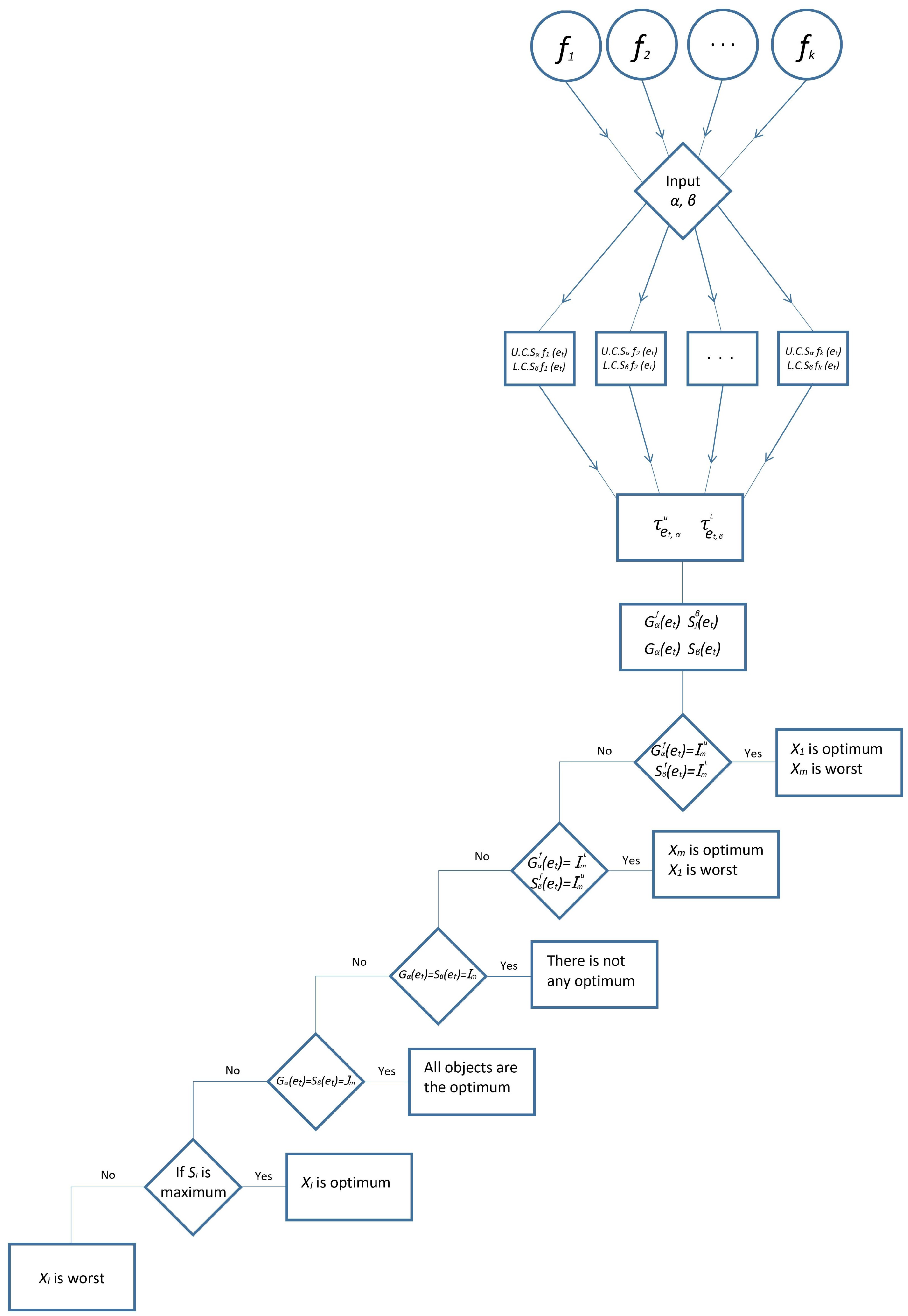
Definition 10.

Let X denote the universal set of objects, E denote the set of parameters, and let the threshold intervals $\alpha ,\beta \subseteq \mathbb{I}$ be given, in which $\alpha =[{\alpha }_1,{\alpha }_1]$ and $\beta =[{\beta }_1,{\beta }_2].$ The mapping $S=X\to \mathbb{R}$ is expressed by

$$\begin{array}{c}\hfill S_i\left(x_i\right)=\sum _{t=1}^n\left(\left[\sum _{j=1}^m{g}_{\alpha }^f{\left(e_t\right)}_{ij}-\sum _{j=1}^m{g}_{\alpha }{\left(e_t\right)}_{ij}\right]-\left[\sum _{j=1}^m{s}_f^{\beta }{\left(e_t\right)}_{ij}-\sum _{j=1}^m{s}_{\beta }{\left(e_t\right)}_{ij}\right]\right),\end{array}$$

(9)

in which $S_i\left(x_i\right)$ is the score function of object $x_i$.

According to this flowchart (see Figure 1), the following algorithm is proposed.

Figure 1. The flowchart for Algorithm 1.

Figure 1. The flowchart for Algorithm 1.

Algorithm 1 Ranking Assessments by Interval-Valued Fuzzy Soft Preorder Relation

Example 1.

Let $X=\{x_1,x_2,x_3,x_4,x_5\}$ denote a set of five-star hotels for one customer and $E=\{e_1,\dots ,e_4\}$ denote a set of parameters. Suppose that customers wish to choose the parameters given by “chromatic exterior and interior design”, “cleanliness”, “facilities”, and “excellent service”, respectively. We can assess the hotels as three $IVFS$ matrices given in the following

Table 1. $f_{1E}$.

${\mathit{f}}_{1\mathit{E}}$	${\mathit{x}}_1$	${\mathit{x}}_2$	${\mathit{x}}_3$	${\mathit{x}}_4$	${\mathit{x}}_5$
$e_1$	$[0.2,0.2]$	$[0.1,0.4]$	$[0.1,0.7]$	$[0.0,0.6]$	$[0.0,0.7]$
$e_2$	$[0.1,0.3]$	$[0.3,0.6]$	$[0.0,0.6]$	$[0.2,0.4]$	$[0.0,0.2]$
$e_3$	$[0.4,0.9]$	$[0.8,1.0]$	$[0.6,0.6]$	$[0.2,0.7]$	$[0.1,0.6]$
$e_4$	$[0.4,0.9]$	$[0.1,0.6]$	$[0.4,0.5]$	$[0.6,0.9]$	$[0.3,0.4]$

,

Table 2. $f_{2E}$.

${\mathit{f}}_{2\mathit{E}}$	${\mathit{x}}_1$	${\mathit{x}}_2$	${\mathit{x}}_3$	${\mathit{x}}_4$	${\mathit{x}}_5$
$e_1$	$[0.0,1.0]$	$[0.6,0.8]$	$[0.2,0.2]$	$[0.2,0.7]$	$[0.1,0.7]$
$e_2$	$[0.3,0.4]$	$[0.1,0.2]$	$[0.5,0.8]$	$[0.2,0.4]$	$[0.1,0.8]$
$e_3$	$[0.3,0.3]$	$[0.1,0.9]$	$[0.2,0.9]$	$[0.7,0.8]$	$[0.3,1.0]$
$e_4$	$[0.1,0.8]$	$[0.1,0.8]$	$[0.5,0.7]$	$[0.1,0.2]$	$[0.3,0.6]$

and

Table 3. $f_{3E}$.

${\mathit{f}}_{3\mathit{E}}$	${\mathit{x}}_1$	${\mathit{x}}_2$	${\mathit{x}}_3$	${\mathit{x}}_4$	${\mathit{x}}_5$
$e_1$	$[0.1,0.5]$	$[0.9,1.0]$	$[0.1,0.3]$	$[0.7,1.0]$	$[0.1,0.5]$
$e_2$	$[0.1,0.4]$	$[0.3,0.8]$	$[0.0,0.4]$	$[0.3,0.5]$	$[0.3,0.4]$
$e_3$	$[0.1,0.3]$	$[0.1,1.0]$	$[0.2,0.6]$	$[0.6,0.9]$	$[0.3,0.9]$
$e_4$	$[0.7,1.0]$	$[0.5,0.6]$	$[0.3,1.0]$	$[1.0,1.0]$	$[0.4,0.5]$

.

Assume that $[{\alpha }_1,{\alpha }_2]=[0.3,0.6]$ and $[\beta ,{\beta }_2]=[0.2,0.4].$

Step $1.$ The upper and lower crisp matrices are given as:

$$f_1=\left[\begin{array}{cccccc}& 0& 0& 0& 0& 0\\ & 0& 0& 0& 0& 0\\ & 1& 1& 0& 0& 0\\ & 1& 0& 0& 0& 0\end{array}\right],f_2=\left[\begin{array}{cccccc}& 0& 1& 0& 0& 0\\ & 0& 0& 1& 0& 0\\ & 0& 0& 0& 1& 0\\ & 0& 0& 1& 0& 0\end{array}\right],f_3=\left[\begin{array}{cccccc}& 0& 1& 0& 1& 0\\ & 0& 0& 0& 0& 0\\ & 0& 0& 0& 1& 0\\ & 1& 0& 0& 1& 0\end{array}\right]$$

$$f_1=\left[\begin{array}{cccccc}& 0& 0& 0& 0& 0\\ & 1& 0& 0& 0& 1\\ & 0& 0& 0& 0& 0\\ & 0& 0& 0& 0& 0\end{array}\right],f_2=\left[\begin{array}{cccccc}& 0& 0& 0& 0& 0\\ & 0& 1& 0& 0& 0\\ & 0& 0& 0& 0& 0\\ & 0& 0& 0& 1& 0\end{array}\right],f_3=\left[\begin{array}{cccccc}& 0& 0& 1& 0& 0\\ & 0& 0& 0& 0& 0\\ & 1& 0& 0& 0& 0\\ & 0& 0& 0& 0& 0\end{array}\right]$$

Step $2.$ The upper and lower topology are expressed in

Table 4. $\alpha$-Upper-$e_t$ topology; $\alpha =[{\alpha }_1,{\alpha }_2],t=1,\dots ,4$.

	${\mathit{\tau }}_{{\mathit{p}}_{\mathit{t}},\mathit{\alpha }}^{\mathit{u}}$
$e_1$	{${\left[0\right]}_{1\times 5}$	${\left[1\right]}_{1\times 5}$	[0	1	0	0	0]	[0	1	0	1	0]}
$e_2$	{${\left[0\right]}_{1\times 5}$	${\left[1\right]}_{1\times 5}$	[0	0	1	0	0] }
$e_3$	{${\left[0\right]}_{1\times 5}$	${\left[1\right]}_{1\times 5}$	[1	1	0	0	0]	[0	0	0	1	0 ]
	[1	1	0	1	0 ] }
$e_4$	{${\left[0\right]}_{1\times 5}$	${\left[1\right]}_{1\times 5}$	[1	0	0	0	0]	[0	0	1	0	0 ]
	[1	0	0	1	0 ]	[1	0	1	0	0 ]
	[1	0	1	1	0 ] }

and

Table 5. $\beta$-Lower-$e_t$ topology; $\beta =[{\beta }_1,{\beta }_2],t=1,\dots ,4$.

	${\mathit{\tau }}_{{\mathit{p}}_{\mathit{t}},\mathit{\beta }}^{\mathit{L}}$
$e_1$	{${\left[0\right]}_{1\times 5}$	${\left[1\right]}_{1\times 5}$	[0	0	1	0	0] }
$e_2$	{${\left[0\right]}_{1\times 5}$	${\left[1\right]}_{1\times 5}$	[1	0	0	0	1]	[0	1	0	0	0]	[1	1	0	0	1]}
$e_3$	{${\left[0\right]}_{1\times 5}$	${\left[1\right]}_{1\times 5}$	[1	0	0	0	0] }
$e_4$	{${\left[0\right]}_{1\times 5}$	${\left[1\right]}_{1\times 5}$	[0	0	0	1	0]}

, accordingly.

Step $3.$ Compute matrices $G_{\alpha }^f\left(e_t\right)$ and $S_{\beta }^f\left(e_t\right)$ by using Equations (5) and (6). Moreover, matrices $G_{\alpha }\left(e_t\right)$ and $S_{\beta }\left(e_t\right)$ are computed using Equations (3) and (4) over $X,$ in which $\alpha =[{\alpha }_1,{\alpha }_2],\beta =[{\beta }_1,{\beta }_2],$ and $t=1,\dots ,4$ given by:

$$G_{\alpha }^f\left(e_1\right)=\left[\begin{array}{cccccc}1& 0& 0& 0& 0& \\ 0& 1& 0& 0& 0& \\ 0& 0& 1& 0& 0& \\ 0& 0& 0& 1& 0& \\ 0& 0& 0& 0& 1& \end{array}\right]S_f^{\beta }\left(e_1\right)=\left[\begin{array}{cccccc}1& 0& 0& 0& 0& \\ 0& 1& 0& 0& 0& \\ 0& 0& 1& 0& 0& \\ 0& 0& 0& 1& 0& \\ 0& 0& 0& 0& 1& \end{array}\right]$$

$$G_{\alpha }^f\left(e_2\right)=\left[\begin{array}{cccccc}1& 0& 0& 0& 0& \\ 0& 1& 0& 0& 0& \\ 0& 0& 1& 0& 0& \\ 0& 0& 0& 1& 0& \\ 0& 0& 0& 0& 1& \end{array}\right]S_f^{\beta }\left(e_2\right)=\left[\begin{array}{cccccc}1& 0& 0& 0& 0& \\ 0& 1& 0& 0& 0& \\ 0& 0& 1& 0& 0& \\ 0& 0& 0& 1& 0& \\ 0& 0& 0& 0& 1& \end{array}\right]$$

$$G_{\alpha }^f\left(e_3\right)=\left[\begin{array}{cccccc}1& 0& 0& 0& 0& \\ 0& 1& 0& 0& 0& \\ 0& 0& 1& 0& 0& \\ 0& 0& 0& 1& 0& \\ 0& 0& 0& 0& 1& \end{array}\right]S_f^{\beta }\left(e_3\right)=\left[\begin{array}{cccccc}1& 0& 0& 0& 0& \\ 0& 1& 0& 0& 0& \\ 0& 0& 1& 0& 0& \\ 0& 0& 0& 1& 0& \\ 0& 0& 0& 0& 1& \end{array}\right]$$

$$G_{\alpha }^f\left(e_4\right)=\left[\begin{array}{cccccc}1& 1& 0& 0& 0& \\ 0& 1& 0& 0& 0& \\ 0& 0& 1& 0& 1& \\ 0& 0& 0& 1& 0& \\ 0& 0& 0& 0& 1& \end{array}\right]S_f^{\beta }\left(e_4\right)=\left(\begin{array}{cccccc}1& 0& 0& 0& 0& \\ 1& 1& 0& 0& 0& \\ 0& 0& 1& 0& 0& \\ 0& 0& 0& 1& 0& \\ 0& 0& 0& 0& 1& \end{array}\right)$$

$$G_{\alpha }\left(e_1\right)=\left[\begin{array}{cccccc}1& 0& 1& 0& 1& \\ 1& 1& 1& 1& 1& \\ 1& 0& 1& 0& 1& \\ 1& 0& 1& 1& 1& \\ 1& 0& 1& 0& 1& \end{array}\right]S_{\beta }\left(e_1\right)=\left[\begin{array}{cccccc}1& 1& 0& 1& 1& \\ 1& 1& 0& 1& 1& \\ 1& 1& 1& 1& 1& \\ 1& 1& 0& 1& 1& \\ 1& 1& 0& 1& 1& \end{array}\right]$$

$$G_{\alpha }\left(e_2\right)=\left[\begin{array}{cccccc}1& 1& 0& 1& 1& \\ 1& 1& 0& 1& 1& \\ 1& 1& 1& 1& 1& \\ 1& 1& 0& 1& 1& \\ 1& 1& 0& 1& 1& \end{array}\right]S_{\beta }\left(e_2\right)=\left[\begin{array}{cccccc}1& 0& 1& 1& 1& \\ 0& 1& 1& 1& 0& \\ 0& 0& 1& 1& 0& \\ 0& 0& 1& 1& 0& \\ 1& 0& 1& 1& 1& \end{array}\right]$$

$$G_{\alpha }\left(e_3\right)=\left[\begin{array}{cccccc}1& 1& 1& 0& 1& \\ 0& 1& 1& 0& 1& \\ 0& 0& 1& 0& 1& \\ 0& 1& 1& 1& 1& \\ 0& 0& 1& 0& 1& \end{array}\right]S_{\beta }\left(e_3\right)=\left[\begin{array}{cccccc}1& 1& 1& 1& 1& \\ 0& 1& 1& 1& 1& \\ 0& 1& 1& 1& 1& \\ 0& 1& 1& 1& 1& \\ 0& 1& 1& 1& 1& \end{array}\right]$$

$$G_{\alpha }\left(e_4\right)=\left[\begin{array}{cccccc}1& 1& 0& 1& 1& \\ 0& 1& 0& 0& 1& \\ 0& 1& 1& 0& 1& \\ 0& 1& 0& 1& 1& \\ 0& 1& 0& 0& 1& \end{array}\right]S_{\beta }\left(e_4\right)=\left(\begin{array}{cccccc}1& 1& 1& 0& 1& \\ 1& 1& 1& 0& 1& \\ 1& 1& 1& 0& 1& \\ 1& 1& 1& 1& 1& \\ 1& 1& 1& 0& 1& \end{array}\right)$$

Step 4. By using Equation (9), in which $\alpha =[{\alpha }_1,{\alpha }_2]$ as well as $\beta =[{\beta }_1,{\beta }_2],$ we have

$$\begin{array}{c}\hfill S_1=r_1(e_1;\alpha ,\beta )+r_1(e_2,\alpha ,\beta )+r_1(e_3,\alpha ,\beta )+r_1(e_4,\alpha ,\beta )=1+2+1+0=4,\end{array}$$

$$\begin{array}{c}\hfill S_2=r_2(e_1;\alpha ,\beta )+r_2(e_2,\alpha ,\beta )+r_2(e_3,\alpha ,\beta )+r_2(e_4,\alpha ,\beta )=-1+(-1)+1+2=1,\end{array}$$

$$\begin{array}{c}\hfill S_3=r_3(e_1;\alpha ,\beta )+r_3(e_2,\alpha ,\beta )+r_3(e_3,\alpha ,\beta )+r_3(e_4,\alpha ,\beta )=2-3+2+1=2,\end{array}$$

$$\begin{array}{c}\hfill S_4=r_4(e_1;\alpha ,\beta )+r_4(e_2,\alpha ,\beta )+r_4(e_3,\alpha ,\beta )+r_4(e_4,\alpha ,\beta )=0-2+0+2=0,\end{array}$$

$$\begin{array}{c}\hfill S_5=r_5(e_1;\alpha ,\beta )+r_5(e_2,\alpha ,\beta )+r_5(e_3,\alpha ,\beta )+r_5(e_4,\alpha ,\beta )=2-1+2+2=5.\end{array}$$

Step 5. Then, the ranking of the overall assessment is obtained as below:

$$x_5⪰x_1⪰x_3⪰x_2⪰x_4.$$

Steps 6 and 7. Therefore, $x_5$ is the best object, while $x_4$ cannot be selected.

5. Conclusions

Fuzzy ordered structures on a universal set are an important research tool to model uncertainty or fuzziness in the real world, which is closely related to fuzzy topology. This paper introduced interval-valued fuzzy soft preorderings, and subsequently an interval-valued fuzzy soft equivalence based on interval-valued fuzzy soft topology. We then presented two different crisp preorderings and equivalence relations over the X-associated interval-valued fuzzy soft topology. Employing a new method for ranking data, a score function was defined to solve multi-group decision-making problems. Finally, a numerical example was given. For future research, interval-valued fuzzy soft ordering is the most powerful concept in system analysis. It can be implemented from the decision-making methods in conflict handling, recommender systems, and practical evaluation systems.

References

1. Zadeh, L.A. Fuzzy Sets. Inf. Control 1965, 8, 338–353. [Google Scholar] [CrossRef] [Green Version]
2. Gorzałczany, M.B. A method of Inference in Approximate Reasoning Based on Interval-Valued Fuzzy Sets. Fuzzy Sets Syst. 1987, 21, 1–17. [Google Scholar] [CrossRef]
3. Atanassov, K.T. Intuitionistic Fuzzy Sets. Fuzzy Sets Syst. 1986, 20, 87–96. [Google Scholar] [CrossRef]
4. Pawlak, Z. Rough Sets. Int. J. Comput. Inf. Sci. 1982, 11, 341–356. [Google Scholar] [CrossRef]
5. Molodtsov, D. Soft Set Theory First Results. Comput. Math. Appl. 1999, 37, 19–31. [Google Scholar] [CrossRef] [Green Version]
6. Maji, P.K.; Biswas, P.; Roy, A.R. A fuzzy Soft Sets. J. Fuzzy Math. 2001, 9, 589–602. [Google Scholar]
7. Roy, A.R.; Maji, P.K. A fuzzy Soft Set Theoretic Approach to Decision Making Problems. J. Comput. Appl. Math. 2007, 203, 412–418. [Google Scholar] [CrossRef] [Green Version]
8. Alcantud, J.C.R. A novel Algorithm for Fuzzy Soft Set Based Decision Making from Multiobserver Input Parameter Data Set. Inf. Fusion 2016, 29, 142–148. [Google Scholar] [CrossRef]
9. Basu, T.M.; Mahapatra, N.K.; Mondal, S.K. A balanced Solution of A fuzzy Soft Set Based Decision Making Problem in Medical Science. Appl. Soft Comput. 2012, 12, 3260–3275. [Google Scholar] [CrossRef]
10. Kong, Z.; Gao, L.; Wang, L. Comment on “A fuzzy Soft Set Theoretic Approach to Decision Making Problems”. J. Comput. Appl. Math. 2009, 223, 540–542. [Google Scholar] [CrossRef] [Green Version]
11. Feng, F.; Jun, Y.B.; Liu, X.; Li, L. An adjustable Approach to Fuzzy Soft Set Based Decision Making. J. Comput. Appl. Math. 2010, 234, 10–20. [Google Scholar] [CrossRef] [Green Version]
12. Alcantud, J.C.R.; Mathew, T.J. Separable Fuzzy Soft Sets and Decision Making with Positive and Negative Attributes. Appl. Soft Comput. 2017, 59, 586–595. [Google Scholar] [CrossRef]
13. Maji, P.K.; Biswas, R.; Roy, A.R. Intuitionistic Fuzzy Soft Sets. J. Fuzzy Math. 2001, 9, 677–692. [Google Scholar]
14. Maji, P.K.; Roy, A.R.; Biswas, R. On Intuitionistic Fuzzy Soft Sets. J. Fuzzy Math. 2004, 12, 669–684. [Google Scholar]
15. Maji, P.K. More on Intuitionistic Fuzzy Soft Sets. In International Workshop on Rough Sets, Fuzzy Sets, Data Mining, and Granular-Soft Computing; Springer: Berlin/Heidelberg, Germany, 2009; pp. 231–240. [Google Scholar]
16. Agarwal, M.; Biswas, K.K.; Hanmandlu, M. Generalized Intuitionistic Fuzzy Soft Sets with Applications in Decision-Making. Appl. Soft Comput. 2013, 13, 3552–3566. [Google Scholar] [CrossRef]
17. Yang, X.; Lin, T.Y.; Yang, J.; Li, Y.; Yu, D. Combination of Interval-Valued Fuzzy Set and Soft set. Comput. Math. Appl. 2009, 58, 521–527. [Google Scholar] [CrossRef] [Green Version]
18. Feng, F.; Li, Y.; Leoreanu-Fotea, V. Application of Level Soft Sets in Decision Making Based on Interval-Valued Fuzzy Soft Sets. Comput. Math. Appl. 2010, 60, 1756–1767. [Google Scholar] [CrossRef] [Green Version]
19. Mondal, T.K.; Samanta, S.K. Topology of Interval-Valued Fuzzy Sets. Indian J. Pure Appl. Math. 1999, 30, 23–29. [Google Scholar]
20. Ali, M.; Kılıçman, A.; Khameneh, A.Z. Separation Axioms of Interval-Valued Fuzzy Soft Topology via Quasi-Neighborhood Structure. Mathematics 2020, 8, 178. [Google Scholar] [CrossRef] [Green Version]
21. Ma, X.; Qin, H.; Sulaiman, N.; Herawan, T.; Abawajy, J.H. The parameter Reduction of the Interval-Valued Fuzzy Soft Sets and its Related Algorithms. IEEE Trans. Fuzzy Syst. 2013, 22, 57–71. [Google Scholar] [CrossRef]
22. Ma, X.; Wang, Y.; Qin, H.; Wang, J. A Decision-Making Algorithm Based on the Average Table and Antitheses Table for Interval-Valued Fuzzy Soft Set. Symmetry 2020, 12, 1131. [Google Scholar] [CrossRef]
23. Ma, X.; Fei, Q.; Qin, H.; Li, H.; Chen, W. A new Efficient Decision Making Algorithm Based on Interval-Valued Fuzzy Soft Set. Appl. Intell. 2021, 51, 3226–3240. [Google Scholar] [CrossRef]
24. Peng, X.; Garg, H. Algorithms for Interval-Valued Fuzzy Soft Sets in Emergency Decision Making Based on WDBA and CODAS with New Information Measure. Comput. Ind. Eng. 2018, 119, 439–452. [Google Scholar] [CrossRef] [PubMed]
25. Wang, L.; Garg, H. Algorithm for Multiple Attribute Decision-Making with Interactive Archimedean Norm Operations Under Pythagorean Fuzzy Uncertainty. Int. J. Comput. Intell. Syst. 2021, 14, 503–527. [Google Scholar] [CrossRef]
26. Khameneh, A.Z.; Kılıçman, A.; Salleh, A.R. An adjustable Approach to Multi-Criteria Group Decision-Making Based on a Preference Relationship under Fuzzy Soft Information. Int. J. Fuzzy Syst. 2017, 19, 1840–1865. [Google Scholar] [CrossRef]
27. Khameneh, A.Z.; Kılıçman, A.; Salleh, A.R. Application of A preference Relationship in Decision-Making Based on Intuitionistic Fuzzy Soft Sets. J. Intell. Fuzzy Syst. 2018, 34, 123–139. [Google Scholar] [CrossRef]
28. Ali, M.; Kılıçman, A.; Zahedi Khameneh, A. Application of Induced Preorderings in Score Function-Based Method for Solving Decision-Making with Interval-Valued Fuzzy Soft Information. Mathematics 2021, 9, 1575. [Google Scholar] [CrossRef]
29. Rajarajeswari, P.; Dhanalakshmi, P. Interval-Valued Fuzzy Soft Matrix Theory. Ann. Pure Appl. Math. 2014, 7, 61–72. [Google Scholar]
30. Basu, T.M.; Mahapatra, N.K.; Mondal, S.K. Matrices in Interval-Valued Fuzzy Soft Set Theory and Their Application. South Asian J. Math. 2014, 4, 1–22. [Google Scholar]