Stability Analysis of Parameter Varying Genetic Toggle Switches Using Koopman Operators

Abstract

The genetic toggle switch is a well known model in synthetic biology that represents the dynamic interactions between two genes that repress each other. The mathematical models for the genetic toggle switch that currently exist have been useful in describing circuit dynamics in rapidly dividing cells, assuming fixed or time-invariant kinetic rates. There is a growing interest in being able to model and extend synthetic biological function for growth conditions such as stationary phase or during nutrient starvation. As cells transition from one growth phase to another, kinetic rates become time-varying parameters. In this paper, we propose a novel class of parameter varying nonlinear models that can be used to describe the dynamics of genetic circuits, including the toggle switch, as they transition from different phases of growth. We show that there exists unique solutions for this class of systems, as well as for a class of systems that incorporates the microbial phenomena of quorum sensing. Further, we show that the domain of these systems, which is the positive orthant, is positively invariant. We also showcase a theoretical control strategy for these systems that would grant asymptotic monostability of a desired fixed point. We then take the general form of these systems and analyze their stability properties through the framework of time-varying Koopman operator theory. A necessary condition for asymptotic stability is also provided as well as a sufficient condition for instability. A Koopman control strategy for the system is also proposed, as well as an analogous discrete time-varying Koopman framework for applications with regularly sampled measurements.

1. Introduction

Switching behavior in biological networks is of interest to many researchers across a variety of disciplines, such as epigenetics [1], synthetic biology [2], dynamical systems [3] and more [4,5,6]. The ability of complex biological networks to implement mixtures of switching behavior and nonlinear smooth system response make them a key area of focus in understanding how network structure, combined with system logic, are able to map structure to function [5,6,7,8]. The toggle switch is a special case of a two node Goodwin oscillator and thus provides the simplest biological realization of multi-stable behavior [9]. Finally, the toggle switch is present as a sub-network motif in many natural biological networks [4].

To date, most synthetic biological circuits are implemented in liquid suspension, assuming well stirred growth conditions and ample nutrient supply. Cells in this setting often divide exponentially, following a log-linear or log-phase growth curve. However, in every batch growth condition, bacterial cells will slowly deplete all nutrients in a growth medium, giving rise to late log-phase or early stationary phase dynamics [10]. In this setting, genetic circuits can be modeled as being subject to time-varying kinetic rates, as the cells are no longer in a state of dynamic, chemical equilibrium. Designing genetic circuits to function in nutrient-limited conditions is an open challenge.

Quorum sensing genes inside of living cells allow the cells to naturally sense when the cell population is becoming increasingly dense, saturating their growth environment, and potentially depleting resources. Quorum sensing genes activate in response to small homoserine lactone molecules, known as quorum signaling molecules, which are produced in cells containing these genes [11]. As the density of the cell population reaches saturation, the fraction of active quorum sensing genes begins to rise, which can act as a natural trigger for late log-phase or stationary phase biological processes. Several ordinary differential equation (ODE) models have been developed to model quorum sensing dynamics [12,13,14]. Nikolaev and Sontag modeled how a network of bacteria such as Pseudomonas fluorescens or E. coli use quorum sensing to synchronize gene expression according to toggle switches within each cell, thus showing how quorum sensing can synchronize switching behavior in a population of cells [15]. Here, we conceptually introduce the phenomenon of quorum sensing; in the sequel we will introduce a toggle switch model with time-varying kinetic rates that explicitly incorporates quorum sensing dynamics. Furthermore, we use quorum sensing in our models because we later implement a control strategy which requires the tracking of cell population density.

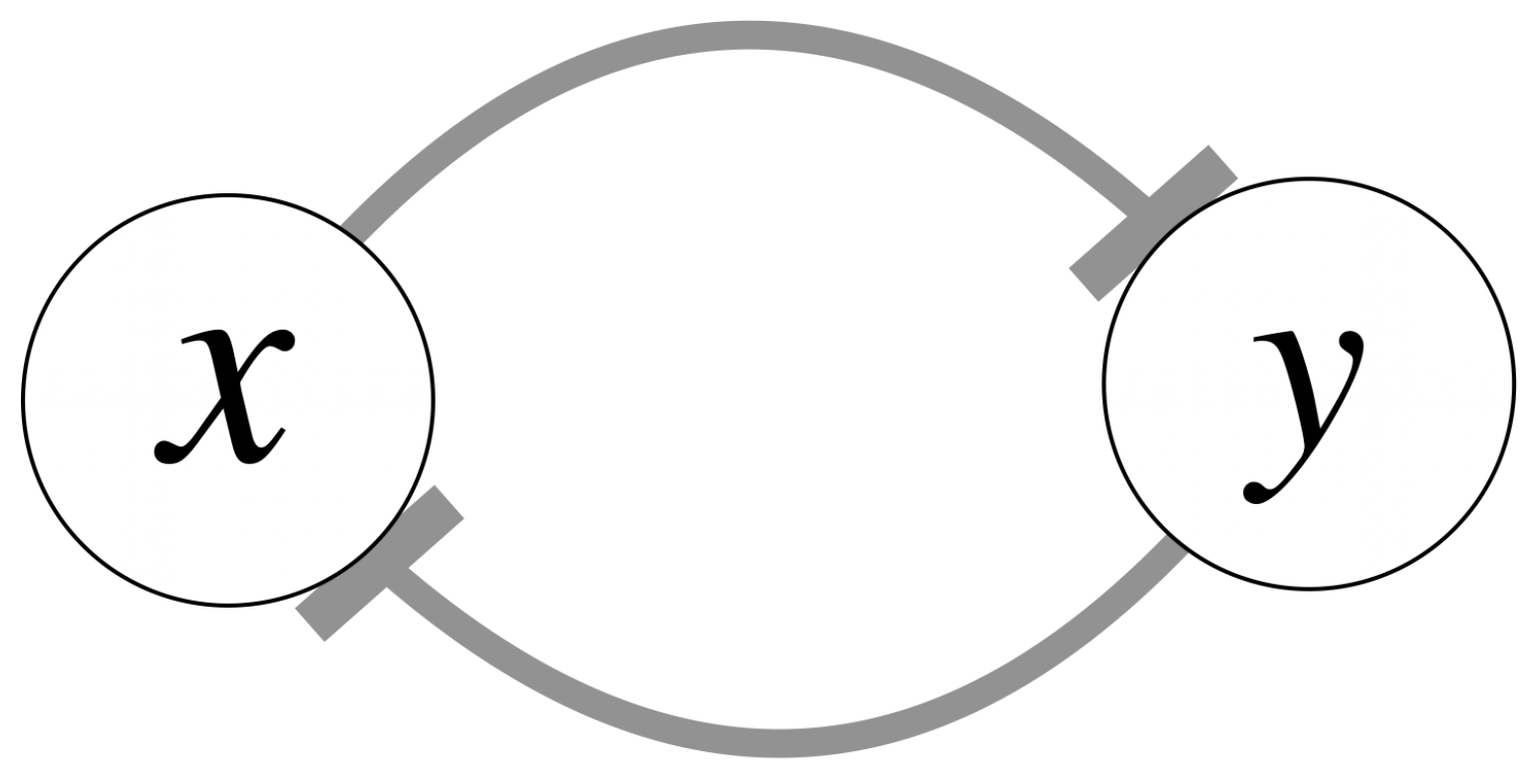
As a brief review, the classical genetic toggle switch [9] is modeled as follows:

$$\dot{x}=\frac{{\alpha }_1}{1+y^{n_y}}-{\delta }_{1}x$$

(1)

$$\dot{y}=\frac{{\alpha }_2}{1+x^{n_x}}-{\delta }_{2}y$$

where $x\in {ℝ}_{\ge 0}$ and $y\in {ℝ}_{\ge 0}$ represent the concentrations of repressor 1 (LacI) and repressor 2 (TetR); ${\alpha }_1$ and ${\alpha }_2$ denote the effective rate of synthesis of repressor 1 and 2; ${\delta }_1>0$ and ${\delta }_2>0$ are the decay rates of repressor 1 and 2 respectively; $n_x\ge 1$ and $n_y\ge 1$ represent the cooperativities of repression of promoter 1 (the Tet promoter) and 2 (the Lac promoter). This formulation can be represented using the standard mutual repression network model in Figure 1.

A feature of the classical genetic toggle switch model is that the parameters are static, i.e., time-invariant. If we relax this assumption for the effective rates of synthesis and the decay rates, then we could have in our model that the kinetic parameters ${\alpha }_1$, ${\alpha }_2$, ${\delta }_1$, ${\delta }_2$ now become time-varying functions, i.e., parameters that change over time. This generalization of the functional form of our system parameters, from time-invariant to time varying, provides a more accurate framework to model the genetic toggle switch in cells transitioning growth phases. Formally, the resulting mathematical model involving the time-varying parameters in question would then be a parameter varying nonlinear system (PVNS). Invoking this idea raises questions related to the stability of such a system as well as transient and steady state behavior. The analysis related to these PVNS toggle switch models is provided in this paper, as well as further findings pertaining to such a system with quorum sensing.

Koopman operator theory has been shown to provide insight into system behavior [16,17,18,19,20,21,22,23] through the analysis of the spectrum of a nonlinear system’s Koopman operator (see Section 3 for a detailed introduction). Specifically, for biological applications, Ref. [24] showed that deep neural networks combined with Koopman operator methods could recover the governing equations of a glycolytic oscillator. Ref. [25] showed that Koopman operators could be used to formulate steady-state control of large-scale biological networks as a data-driven convex program, while Ref. [26] showed that cell growth could be modeled and predicted using Koopman operators that acted on temporal embeddings. Hasnain et al. [27] subsequently demonstrated that dynamic mode decomposition, a numerical method for estimating linear Koopman operators, could be used to quantify the impact of synthetic gene dynamics on a host organism. For observability and state estimation, Ref. [28] showed that Koopman operator methods could be used to determine sensor placement in sparsely measured gene networks and Ref. [26] showed that sensor fusion with Koopman operators enables more accurate identification of the underlying embedding space of Koopman observables.

Most recently, Johnson [29] showed that multi-stability of the genetic toggle switch can be successfully recapitulated with a special basis of Koopman observables that satisfied approximate closure. Nandanoori [30] showed that the spectrum of the genetic toggle switch’s Koopman operator can be decomposed to mirror the invariant subspaces of the original toggle switch’s phase space. In the literature described above, models of the toggle switch, or more generally, the biological network of interest assumed that cells were in a single growth phase, namely exponential growth phase. Motivated by the parameter-varying nature of growth-phase transitions, here we define and extend the Koopman operator framework for the analysis of parameter varying nonlinear system models.

2. Parameter Varying Toggle Switch Models

2.1. Parameter-Varying Toggle Switch (PVTS) System Model

The need for time-varying kinetic rates in the genetic toggle switch model comes from the current inability to model and extend synthetic biological function to growth conditions such as stationary phase or during nutrient starvation. With this quality in mind, the expression of the two genes of the toggle switch in the given organism can then be represented by the following parameter-varying nonlinear system.

$$\left(\begin{array}{c}\dot{x}\\ \dot{y}\end{array}\right)=\left(\begin{array}{c}\frac{{\alpha }_1(t)}{1+{(y/k_y)}^{n_y}}-{\delta }_1(t)x\\ \frac{{\alpha }_2(t)}{1+{(x/k_x)}^{n_x}}-{\delta }_2(t)y\end{array}\right)$$

(2)

where $x\in {ℝ}_{\ge 0}$, $y\in {ℝ}_{\ge 0}$ represent the concentrations of repressor one and repressor two; ${\alpha }_1(t)>0$ and ${\alpha }_2(t)>0$ denote the effective rates of synthesis of repressor one and two. Note that we also require ${\alpha }_1(t)$ and ${\alpha }_2(t)$ to be bounded and to converge to positive constants; ${\delta }_1(t)>0$ and ${\delta }_2(t)>0$ are the self decay rates of repressor one, repressor two. Further, we note the requirement that ${\delta }_1(t)$ and ${\delta }_2(t)$ are bounded and converge to positive constants. The constants $n_x\ge 1$ and $n_y\ge 1$ represent the respective cooperativities of repression for promoter one and promoter 2; the Michaelis constants $k_x$ and $k_y$ are respective binding affinities. Similar to (1), we have that $(x,y)\in {ℝ}_{\ge 0}\times {ℝ}_{\ge 0}$, i.e., the system is assumed to operate on the positive orthant.

Given that ${\alpha }_1(t),{\alpha }_2(t)$ are strictly positive functions over time, this is a parameter varying nonlinear system of the general form:

$$\dot{\overrightarrow{x}}=\overrightarrow{f}(\overrightarrow{x}(t),\overrightarrow{\alpha }(t),\overrightarrow{\delta }(t))$$

(3)

where $\overrightarrow{\alpha }(t)$ and $\overrightarrow{\delta }$ are the vectors of time-varying parameters

$$\overrightarrow{\alpha }(t)=\left(\begin{array}{c}{\alpha }_1(t)\\ {\alpha }_2(t)\end{array}\right),\overrightarrow{\delta }(t)=\left(\begin{array}{c}{\delta }_1(t)\\ {\delta }_2(t)\end{array}\right)$$

and $\overrightarrow{x}\in {\mathbb{R}}^2$, $t\ge 0$, $\overrightarrow{f}:{\mathbb{R}}^2\to {\mathbb{R}}^2.$ As a modelling choice, it makes sense to assume that our time-varying parameters are bounded because it would be physically improbable for there to be an unbounded rate of synthesis in $\overrightarrow{\alpha }(t)$ or an unbounded rate of decay in $\overrightarrow{\delta }(t)$. Furthermore, asserting these natural assumptions of boundedness will guarantee existence and uniqueness of solutions for this model (see Appendix A), which has already been established for the standard genetic toggle switch model.

This model is flexible in that $\overrightarrow{\alpha }(t),\overrightarrow{\delta }(t)$ can be chosen to be sets of natural endogenous kinetic rates or to be sets of expression rate multipliers. As measurement technologies of kinetic rates in synthetic biology advance, it may be appropriate to select our time-varying parameters to be piecewise continuous functions, producing a piecewise smooth hybrid dynamical system, or to identify these parameter functions in a data-driven fashion. For the purposes of this paper, we will simply assume positivity, convergence to a positive constant, and boundedness.

Promoter leakiness has been modeled with the inclusion of time-invariant parameters which have been shown to affect stability properties of genetic toggle switches [31]. It is important to note that these parameters can be included in our models as multiplicative constants contained in the time-varying parameters and constant affine linear inputs. Using time-varying parameters to model resource usage is in contrast to other contemporary modeling approaches which use time-invariant parameters and a restructuring of the vector field [31].

Our models assume a negligible amount of cellular heterogeneity, as cellular heterogeneity would invoke the use of stochastic methods to model parameters [31]. This assumption holds when modeling bulk or average cell dynamics in batch or batch-fed reactor growth conditions; our framework thus is relevant for these physiological growth conditions. We remark that stochastic single-cell analysis with Koopman operator methods is beyond the scope of this paper and remains the subject of future studies.

With a defined model class and physiologically motivated collection of assumptions, one important modeling criterion is that the generalized set of toggle switch equations should have unique solutions for the initial conditions on the domain. If we have an ODE of the form $\dot{\overrightarrow{x}}(t)=\overrightarrow{f}(\overrightarrow{x},t)$ where $\overrightarrow{f}(\overrightarrow{x},t)$ is Lipschitz over some domain $\mathcal{D}$ in $\overrightarrow{x}$ with $t\ge t_0$, then we have existence and uniqueness of solutions to the initial value problem with initial conditions starting in $\mathcal{D}$ [32].

Since the classical genetic toggle switch has been shown to have unique solutions over its domain, then our more generalizing system should share this trait. This is given by Proposition 1 where the proof can be found in Appendix A.

Proposition 1.

Solutions to the PVTS with initial conditions ${\overrightarrow{x}}_0$ starting in $\mathcal{D}={ℝ}_{\ge 0}\times {ℝ}_{\ge 0}$ exist and are unique for $t\ge 0$.

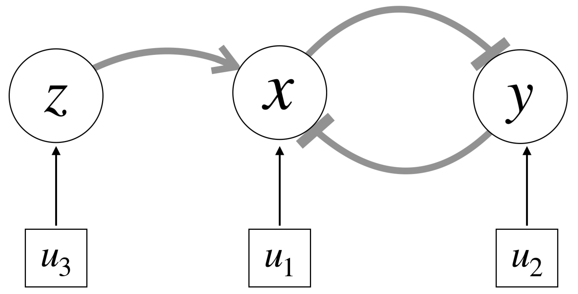
2.2. Genetic Toggle Switch with Quorum Sensing

Cells with quorum sensing genes are able to regulate their gene expression based on the density of the cell population. We model the genetic toggle switch with quorum sensing (GTSQS) by incorporating the quorum sensing components of the genetic circuit using a 3rd state z that activates the first state x via a standard activator. The quorum sensing element $u_3$ will feed into this activator linearly, as will the respective inducers $u_1$ and $u_2$ of the two genes of the toggle switch x and y (see Figure 2 for a network diagram).

The mathematical model of such a system is as follows:

$$\left(\begin{array}{c}\dot{x}\\ \dot{y}\\ \dot{z}\end{array}\right)=\left(\begin{array}{c}\frac{{\alpha }_1(t){(z/k_z)}^{n_z}}{1+{(y/k_y)}^{n_y}+{(z/k_z)}^{n_z}}-{\delta }_1(t)x\\ \frac{{\alpha }_2(t)}{1+{(x/k_x)}^{n_x}}-{\delta }_2(t)y\\ \frac{{\alpha }_3(t)z}{k_z+z}-{\delta }_3(t)z\end{array}\right)+\left(\begin{array}{c}{u}_1(t)\\ u_2(t)\\ u_3(t)\end{array}\right)$$

(4)

where x, y represent the concentrations of repressor 1 and repressor 2; z represents the quorum sensing activation response of the system that ultimately affects the concentrations x and y; ${\alpha }_1(t)>0$ and ${\alpha }_2(t)>0$ denote the effective rates of synthesis of repressor 1 and 2, respectively; ${\alpha }_3(t)>0$ denotes the effective rate of the quorum sensing activator i.e., the rate at which quorum sensing affects gene expression; ${\delta }_i(t)>0,i\in \{1,2,3\}$ are the self decay rates of repressor 1, repressor 2, and the quorum sensing input, respectively; $n_{x,y,z}\ge 1$ represent the cooperativities of repression of promoter 1, promoter 2, and the quorum sensing input, respectively; $k_{x,y,z}>0$ are the respective binding affinities; $(x,y,z)\in {ℝ}_{\ge 0}\times {ℝ}_{\ge 0}\times {ℝ}_{\ge 0}$; $u_1,u_2$ are the inducers modeled as affine linear inputs; $u_3$ is the quorum sensing input. Note that we also require the time-varying parameters to be bounded functions of time which converge to positive constants.

In general, input signals to a biological network enter a nonlinear term, but the overall input signal may be generated by a Hill function [4]. Usually these input functions describe substrate saturation of a small molecule diffusing the cell membrane or a small molecule of mRNA designed to create interference, e.g., a CRISPRi gRNA designed to repress expression of a gene. In such a setting, there is always additive separability and so a generic input signal $u(t)$ can be defined as the functional value of each of these nonlinear saturation functions. In short, this justifies the use of additive, linear input terms, even if the underlying substrate used to drive the control of the system may be subject to saturation. Further, for defined windows of input concentration, we can also argue that the inputs are approximately linear, when well within the windows of saturation.

This leads us to a GTSQS system of the form:

$$\dot{\overrightarrow{x}}(t)=\overrightarrow{f}(\overrightarrow{x},t)+\overrightarrow{u}(t)$$

(5)

where

$$\overrightarrow{f}(\overrightarrow{x},t)=\left(\begin{array}{c}\frac{{\alpha }_1(t){(z/k_z)}^{n_z}}{1+{(y/k_y)}^{n_y}+{(z/k_z)}^{n_z}}-{\delta }_1(t)x\\ \frac{{\alpha }_2(t)}{1+{(x/k_x)}^{n_x}}-{\delta }_2(t)y\\ \frac{{\alpha }_3(t)z}{k_z+z}-{\delta }_3(t)z\end{array}\right)$$

and $\overrightarrow{u}(t)={(u_1(t),u_2(t),u_3(t))}^T$. More generally, it is a parameter varying nonlinear system of the form:

$$\dot{\overrightarrow{x}}=\overrightarrow{f}(\overrightarrow{x},\overrightarrow{\alpha }(t),\overrightarrow{\delta }(t)\overrightarrow{u}(t))$$

(6)

where

$$\overrightarrow{\alpha }(t)=\left(\begin{array}{c}{\alpha }_1(t)\\ {\alpha }_2(t)\\ {\alpha }_3(t)\end{array}\right),\overrightarrow{\delta }(t)=\left(\begin{array}{c}{\delta }_1(t)\\ {\delta }_2(t)\\ {\delta }_3(t)\end{array}\right)$$

and $\overrightarrow{x}\in {ℝ}^3$.

We present the system (7) below to showcase an example of GTSQS behavior.

$$\left(\begin{array}{c}\dot{x}\\ \dot{y}\\ \dot{z}\end{array}\right)=\left(\begin{array}{c}\frac{(1+e^{-t})z}{1+y^{2.5}+z}-\left(\frac{1}{2+e^{-t}}\right)x\\ \frac{(1+e^{-t})}{1+x^{2.5}}-\left(\frac{1}{2+e^{-t}}\right)y\\ \frac{(1+e^{-t})z}{1+z}-\left(\frac{1}{2+e^{-t}}\right)z\end{array}\right)+\left(\begin{array}{c}{u}_1\\ u_2\\ u_3\end{array}\right)$$

(7)

For clarity, system (7) is the system (5) with the following parameters.

$$\begin{array}{cc}\hfill & {\alpha }_1(t)={\alpha }_2(t)={\alpha }_3(t)=(1+e^{-t})\hfill \\ \hfill & {\delta }_1(t)={\delta }_2(t)={\delta }_3(t)={(2+e^{-t})}^{-1}\hfill \\ \hfill & n_x=n_y=2.5,n_z=1\hfill \\ \hfill & k_x=k_y=k_z=1.\hfill \end{array}$$

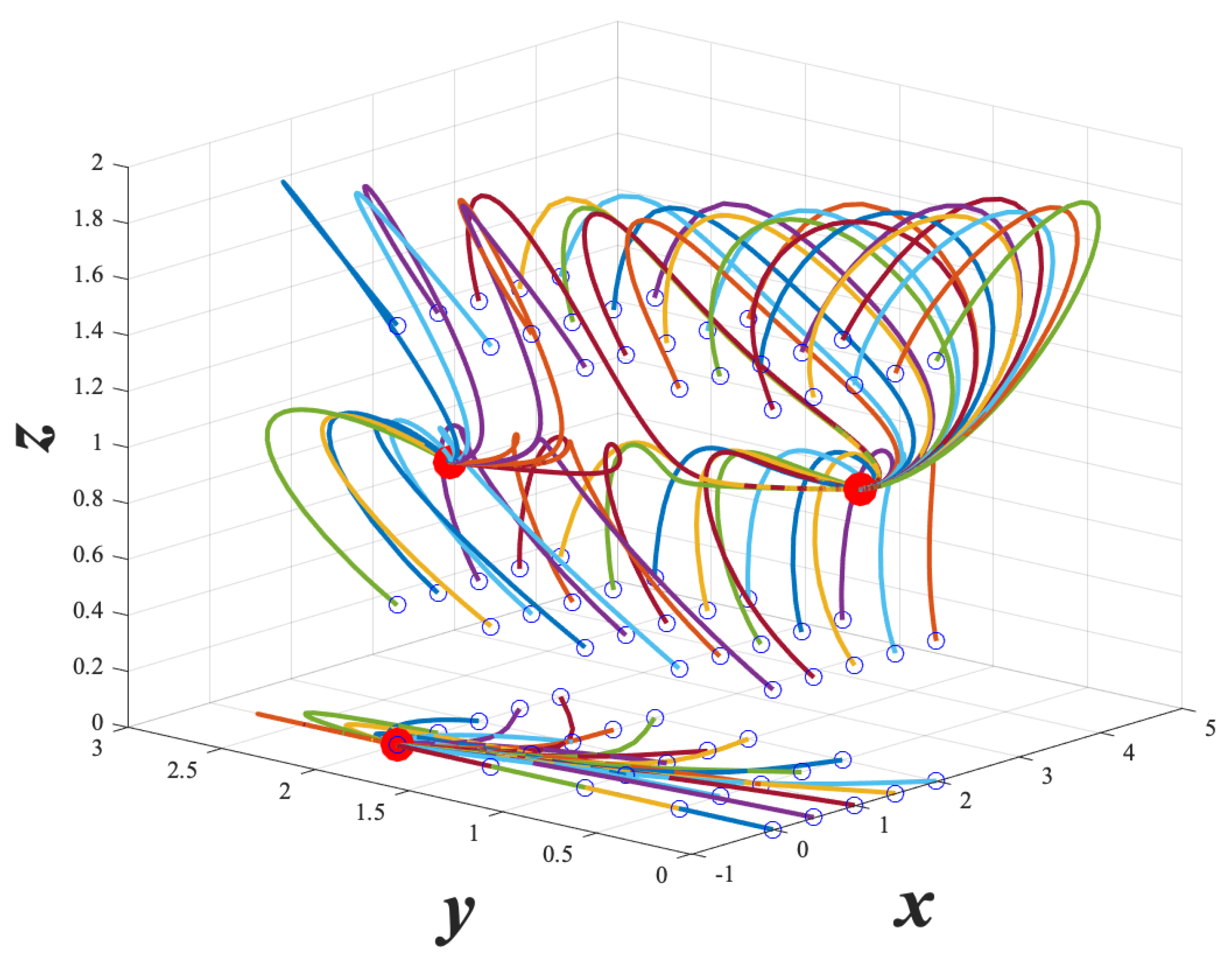
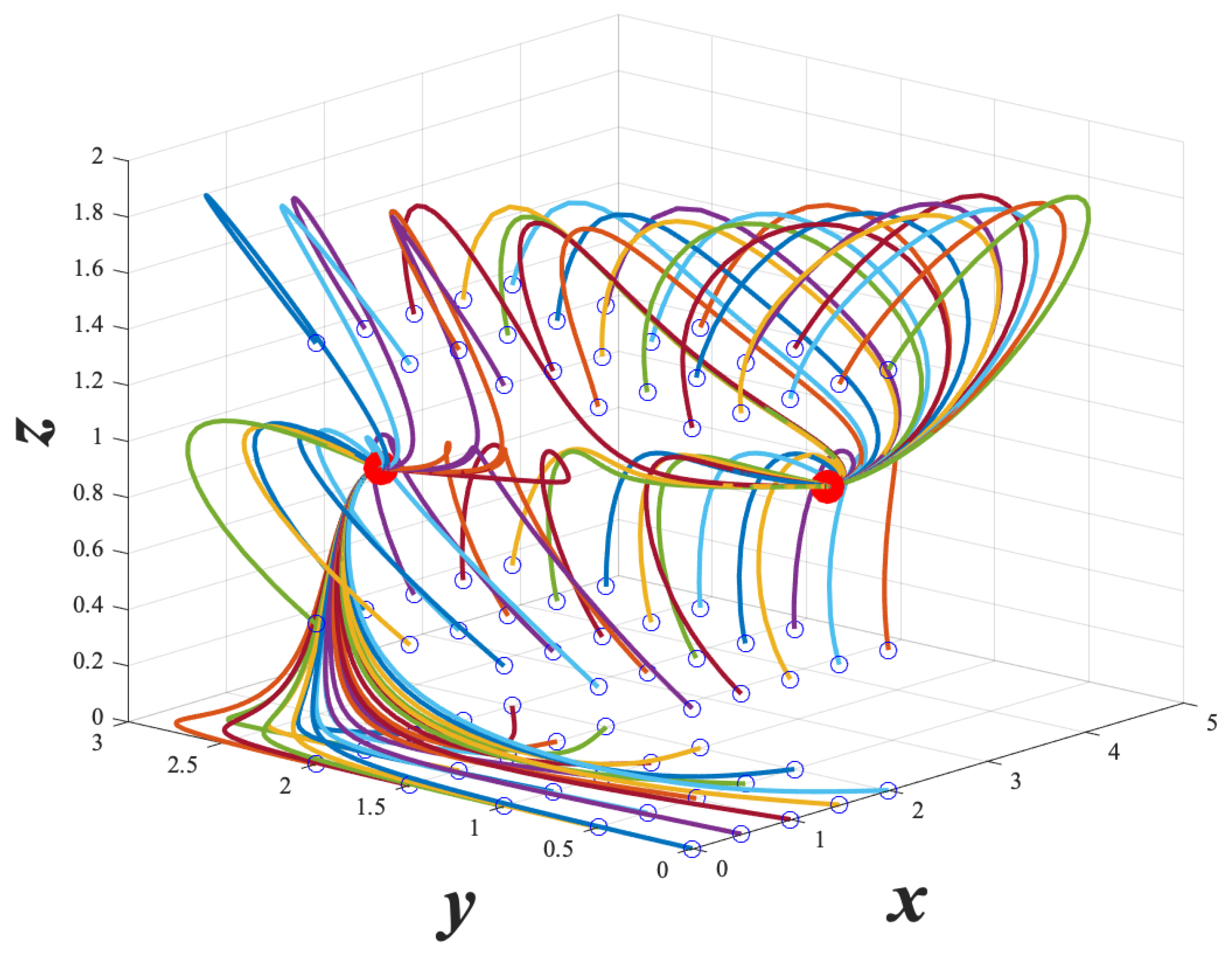
In this example, our time-varying parameters elicit gene expression responses we would expect in the context of nutrient starvation. On the time interval $t\in [0,\infty )$, we see that our functions in $\overrightarrow{\alpha }(t)$ go from $2\to 1$ and our functions in $\overrightarrow{\delta }(t)$ go from $\frac{1}{3}\to \frac{1}{2}$ as t goes from $0\to \infty$. Intuitively, this means that the rates of synthesis are decreasing while the rates of decay are increasing. Furthermore, they satisfy our modeling requirements in that the functions are continuous, bounded, and exist in the limit as $t\to \infty$.

From Figure 3 and Figure 4 below, we can visualize the dynamics of example system (7), and get a brief intuition of the behavior of the GTSQS. We see in Figure 3 that the $z=0$ plane is invariant, and there is one stable fixed point on this plane. We also see that for initial conditions with $z>0$, go to one of two stable fixed points. Figure 4 shows that given a quorum sensing input $u_3=0.01$, we can take the initial conditions in the $z=0$ plane to one of the other fixed points. In this way, our model captures how quorum sensing can affect log-phase and stationary phase gene expression.

2.3. Analysis of GTSQS Model

Here we provide mathematical analysis of our model over the domain $\mathcal{D}$ which is the first octant:

$$\mathcal{D}=\{(x,y,z)|x\ge 0,y\ge 0,z\ge 0\}.$$

The motivation for the choice of the domain of the GTSQS is that physically, it would be impossible for the state variables $x,y,z$ (which represent quantities correlated to gene expression) to be negative in the sense of physical reality. Therefore, our model should not allow our state variables to be negative if we want the model to reflect biological phenomena. If one would like to experiment with possible negative states (outside the scope of this paper), then one should keep in mind that certain choices of $n_x,n_y,n_z$ may result in a vector field that have non-zero imaginary part, and inquiry into this topic would require tools from complex analysis.

2.3.1. Positively Invariant Domain

It can be trivially shown that for the genetic toggle switch (1) and for the PVTS (2) the first quadrant is positively invariant. Since this is the case, we require a similar result for our generalized model that is the GTSQS (4). We provide this result along with a proof that should serve as the blueprint for showing that the first quadrant is positively invariant for the systems (1) and (2).

Theorem 1.

The positive orthant is positively invariant under the flow of the GTSQS with no inputs.

Proof. 

We want to show that the domain:

$$\mathcal{D}=\{(x,y,z)|x\ge 0,y\ge 0,z\ge 0\}$$

is positively invariant under the flow of the autonomous GTSQS, that is, $(x(t),y(t),z(t))\in \mathcal{D}$ for all $t\ge 0$ if $(x_0,y_0,z_0)\in \mathcal{D}$, and $\overrightarrow{u}=0$.

We start our proof by assuming, for contradiction, that the system is not positively invariant, i.e., that for some $(x_0,y_0,z_0)\in \mathcal{D}$, $(x(t),y(t),z(t))\notin \mathcal{D}$ for some $t\ge 0$. In order for this to be the case, the trajectory $(x(t),y(t),z(t))$ must have passed through the boundary of the first octant ${\mathcal{D}}_B=\{(0,y,z)\}\cup \{(x,0,z)\}\cup \{(x,y,0)\}$ Plugging in these boundary coordinates to the dynamics of our system, it is clear that if $x=0$, then $\dot{x}\ge 0$; if $y=0$, then $\dot{y}\ge 0$; if $z=0$, then $\dot{z}\ge 0$ which implies that our trajectory could not have left $\mathcal{D}$. □

Remark 1.

We verify only for the $u=0$ case because it is always mathematically possible to select some input u that would bring our state out of the positive orthant, even if such a control input would not be feasible in an actual genetic circuit.

2.3.2. Existence of Unique Solutions of GTSQS

In order to show that the GTSQS meets some basic criteria, and is in line with existing genetic toggle switch theory, we provide Proposition 2 to ensure that our model has unique solutions on our domain (proof found in Appendix B).

Proposition 2.

Solutions to the GTSQS with initial conditions ${\overrightarrow{x}}_0$ starting in

$$\mathcal{D}={ℝ}_{\ge 0}\times {ℝ}_{\ge 0}\times {ℝ}_{\ge 0}$$

exist and are unique assuming bounded time-varying parameters where $t\ge 0$.

2.3.3. Controllability of GTSQS

One of the properties to consider when designing a control system is controllability of the domain. In this section we see that the domain of the GTSQS is in fact controllable using the feedback linearization control strategy as follows:

We can write the GTSQS as

$$\left(\begin{array}{c}\dot{x}\\ \dot{y}\\ \dot{z}\end{array}\right)=\left(\begin{array}{c}{\alpha }_1(t)f_1(y,z)-{\delta }_1(t)x\\ {\alpha }_2(t)f_2(x)-{\delta }_2(t)y\\ {\alpha }_3(t)f_3(z)-{\delta }_3(t)z\end{array}\right)+\left(\begin{array}{c}{u}_1(t)\\ u_2(t)\\ u_3(t)\end{array}\right)$$

(8)

where

$$\begin{array}{cc}\hfill f_1(y,z)& =\frac{{\alpha }_1(t){(z/k_z)}^{n_z}}{1+{(y/k_y)}^{n_y}+{(z/k_z)}^{n_z}}\hfill \\ \hfill f_2(x)& =\frac{{\alpha }_2(t)}{1+{(x/k_x)}^{n_x}}\hfill \\ \hfill f_3(z)& =\frac{{\alpha }_3(t)z}{k_z+z}\hfill \end{array}$$

and we choose the controller $u(t)$ such that

$$\left(\begin{array}{c}{u}_1(t)\\ u_2(t)\\ u_3(t)\end{array}\right)=\left(\begin{array}{c}-{\alpha }_1(t)f_1(y,z)+{\overline{u}}_1\\ -{\alpha }_2(t)f_2(x)+{\overline{u}}_2\\ -{\alpha }_3(t)f_3(z)+{\overline{u}}_3\end{array}\right)$$

where ${\overline{u}}_1$, ${\overline{u}}_2$, ${\overline{u}}_3$ are chosen to get desired steady state values. This implies that the system under the described control input has the desired GAS fixed point

$$(x^{\ast },y^{\ast },z^{\ast })=\left(\frac{{\overline{u}}_1}{{\overline{\delta }}_1},\frac{{\overline{u}}_2}{{\overline{\delta }}_2},\frac{{\overline{u}}_3}{{\overline{\delta }}_3}\right).$$

where ${\overline{\delta }}_i$ is respective limit of ${\delta }_i(t)$ as $t\to \infty$ for all $i\in \{1,2,3\}$. Since the desired fixed point can be chosen to be any point in our domain $\mathcal{D}$, the system is controllable. Furthermore, since the controlled system is linear, the fixed point is unique, whereas the system with no input usually has more depending on the choice of parameters.

This mathematical result from feedback linearization is not robust. We only showcase the rudimentary controller above to show that the system is in fact theoretically controllable. In order for this control law to work in practice, one must be completely accurate in capturing the nonlinearities and time-varying parameters in $u(t)$, which is a non-trivial endeavor [32]. Hoping that this would work in a real genetic toggle switch is optimistic at best and a robust control strategy is required. The developments that have been made in the field of robust control allow us to synthesize theoretical controllers for this class of systems that give desired system behavior [33].

3. Stability Analysis of Parameter-Varying Nonlinear Systems with a Koopman Operator Approach

We now consider stability analysis of the genetic toggle switch, using a more general method that applies to a broader class of parameter-varying nonlinear systems. To begin, notice that the genetic toggle switch model with quorum sensing (2) can be written as

$$\dot{\overrightarrow{x}}=A(t)\overrightarrow{f}(\overrightarrow{x})-\Delta (t)\overrightarrow{x}$$

(9)

with the following assumptions:

$$\begin{array}{ll}A(t)\hfill & =\left(\begin{array}{cccc}{\alpha }_{11}(t)& \cdots & \cdots & {\alpha }_{1n}(t)\\ {\alpha }_{21}(t)& \ddots & & ⋮\\ ⋮& & \ddots & {\alpha }_{n-1,n}(t)\\ {\alpha }_{n1}(t)& \cdots & \cdots & {\alpha }_{nn}(t)\end{array}\right),\hfill \\ \overrightarrow{f}(\overrightarrow{x})\hfill & =\left(\begin{array}{c}{f}_1(\overrightarrow{x})\\ ⋮\\ f_n(\overrightarrow{x})\end{array}\right),\hfill \\ \Delta (t)\hfill & =\left(\begin{array}{cccc}{\delta }_{11}(t)& \cdots & \cdots & {\delta }_{1n}(t)\\ {\delta }_{21}(t)& \ddots & & ⋮\\ ⋮& & \ddots & {\delta }_{n-1,n}(t)\\ {\delta }_{n1}(t)& \cdots & \cdots & {\delta }_{nn}(t)\end{array}\right),\hfill \end{array}$$

and $\overrightarrow{f}:{ℝ}^n\to {ℝ}^n$ is a vector-valued analytic function, $A(t)$ and $\Delta (t)$ are positive (all entries greater than zero for all t), bounded, continuous time-varying parameter matrices which converge to positive constant matrices in the limit as $t\to \infty$.

Remark 2.

If one wishes to analyze the general form of the system in (9) or to look at a particular case of an example system by choosing parameters, take precaution in removing the assumptions established as you may not be able to guarantee that the initial value problem for (9) has unique solutions.

Parameter-varying nonlinear systems of this form have multiplicatively separable structure; the term $A(t)\overrightarrow{f}(\overrightarrow{x})$ describes generalized birth processes in the creation of states while the term $-\Delta (t)\overrightarrow{x}$ describes generalized death processes. Both birth and death processes are attenuated or adjusted as a function of time, but the attenuation terms $A(t)$ and $\Delta (t)$ may be independent and distinct for birth and death processes, respectively. As described previously, a strong motivation for systems with this structure is the presence of time-dependent kinetic rates in many biological reactions in living cells [10]. The assumptions previously stated allow us to arrive at conclusions that cater to these physical models of interest, while the most general form of results fall fairly directly from established theory on linear time-varying (LTV) systems [34].

Our first goal is to develop a generalized method to analyze the stability of this system. Direct analysis of a standard ansatz Lyapunov function such as $V(\overrightarrow{x})={\overrightarrow{x}}^T\overrightarrow{x}$ can yield nice results, but in general, coming up with Lyapunov functions for stability is a nontrivial endeavor. We seek to extend the characterizations of stability from LTV theory to a broader class of nonlinear parameter varying systems that have the structure of Equation (9). To achieve this goal we will introduce and extend the method of Koopman to this class of parameter varying nonlinear systems because there has been much work done on the stability of nonlinear systems within this framework [19,35,36,37,38]. First, we briefly introduce the Koopman operator representation of a time-invariant dynamical system.

Suppose that

$$\frac{d\overrightarrow{x}}{dt}=\overrightarrow{f}(\overrightarrow{x})$$

(10)

is a continuous time nonlinear dynamical system. There exists an infinite-dimensional linear operator $U_t$ that acts on a Hilbert function space $\mathcal{G}$ with invariant measure $\mu$ to satisfy the equation

$$\frac{d\overrightarrow{g}(\overrightarrow{x}(t))}{dt}=\mathcal{K}\circ \overrightarrow{g}(\overrightarrow{x}(t))$$

(11)

where $\mathcal{K}$ is known as a Koopman generator for the system (10), with corresponding Koopman observable $\overrightarrow{g}(\overrightarrow{x})$. In general, the Koopman generator admits an uncountable spectra, as it operates on an infinite dimensional function space. In special cases, say for when $\overrightarrow{f}(\overrightarrow{x})$ is analytic, then the Koopman generator can be countably infinite dimensional or finite dimensional. The Koopman generator obtains its namesake in that it is used to generate a semigroup of flows on the state of the system, parameterized by the time variable t. In particular, when treating continuous time-invariant dynamical systems, we say that the Koopman generator generates a semigroup of Koopman operators [18].

$${\mathbf{U}}_t=\{exp\circ (\mathcal{K}t)\}.$$

Any element $U_t\in {\mathbf{U}}_t$ acts on the Koopman observable $g({\overrightarrow{x}}_0)$, evaluated at some initial condition ${\overrightarrow{x}}_0$, to give $\overrightarrow{g}(\overrightarrow{x}(t))$ at time $t\in [0,\infty )$. These elements $U_t$ are known as continuous-time Koopman operators that determine the flow of the dynamical system mapped through the Koopman observable $\overrightarrow{g}(\overrightarrow{x}(t))$, as opposed to the direct flow of the dynamical system in its natural state space [20].

The observable function $\overrightarrow{g}(\overrightarrow{x}(t))$ is the element of a function space $\mathcal{G}$, which can be a function space of vector-valued, scalar-valued, matrix valued functions, etc. There are often multiple function spaces and multiple choices of Koopman observables that are consistent with an operator $U_t$ to satisfy the Koopman generator Equation (11), but a particular class of Koopman observables of interest are state-inclusive or state-recoverable Koopman observables [17,39,40,41,42,43]. Such Koopman observables $g(\overrightarrow{x}(t))$ satisfy the property that there exists some function $\overrightarrow{P}:\mathcal{G}\to {\mathbb{R}}^n$ such that $\overrightarrow{x}(t)=\overrightarrow{P}(\overrightarrow{g}(\overrightarrow{x}(t)))$. An example of this is the class of Koopman observables where $\overrightarrow{g}(\overrightarrow{x})$ is a vector valued function of the form

$$\overrightarrow{g}(\overrightarrow{x})=\left(\begin{array}{c}\overrightarrow{x}\\ \overrightarrow{\phi }(\overrightarrow{x})\end{array}\right)$$

(12)

which is called a state inclusive Koopman observable. The nonlinear Koopman observables are held in $\overrightarrow{\phi }(\overrightarrow{x})$ while the state of the system $\overrightarrow{x}$ is also used as an observable in $\overrightarrow{g}(\overrightarrow{x})$. The standard case of Koopman observables which is not state-inclusive is just $\overrightarrow{g}(\overrightarrow{x})=\overrightarrow{\phi }(\overrightarrow{x})$ [41]. The application problem often informs the appropriate function space for the Koopman observable.

3.1. State Inclusive Time-Invariant Koopman Learning

It is of interest to investigate the Koopman learning problem of Equation (9) which is a time-varying nonlinear system. Before we do this, let us cover the framework for state inclusive time-invariant Koopman Learning found in [39].

We begin with a nonlinear system of the form

$$\dot{\overrightarrow{x}}=\overrightarrow{f}(\overrightarrow{x})$$

(13)

and we choose our state-inclusive set of observables $\overrightarrow{g}(\overrightarrow{x})=\left(\begin{array}{c}\overrightarrow{x}\\ \overrightarrow{\phi }(\overrightarrow{x})\end{array}\right)$ such that

$$\dot{\overrightarrow{x}}=K_{xx}\overrightarrow{x}+K_{x\phi }\overrightarrow{\phi }(\overrightarrow{x})$$

(14)

and

$$\dot{\overrightarrow{\phi }}(\overrightarrow{x})=K_{\phi x}\overrightarrow{x}+K_{\phi \phi }\overrightarrow{\phi }(\overrightarrow{x})$$

(15)

which converts the system into the linear form:

$$\left(\begin{array}{c}\dot{\overrightarrow{x}}\\ \dot{\overrightarrow{\phi }}\end{array}\right)=\underset{K}{\underbrace{\left(\begin{array}{cc}{K}_{xx}& K_{x\phi }\\ K_{\phi x}& K_{\phi \phi }\end{array}\right)}}\left(\begin{array}{c}\overrightarrow{x}\\ \overrightarrow{\phi }(\overrightarrow{x})\end{array}\right)$$

(16)

Note that here, we see that

$$\begin{array}{c}\hfill K_{xx}\mathrm{is}\mathrm{a}n\times n\mathrm{matrix}\\ \hfill K_{x\phi }\mathrm{is}\mathrm{a}n\times m\mathrm{matrix}\\ \hfill K_{\phi x}\mathrm{is}\mathrm{a}m\times n\mathrm{matrix}\\ \hfill K_{\phi \phi }\mathrm{is}\mathrm{a}m\times m\mathrm{matrix}\end{array}$$

If $m<\infty$, then the matrix K is finite-dimensional for the chosen set of observables $\overrightarrow{\phi }(\overrightarrow{x})$. In this case, we say that the basis of observables $\overrightarrow{\phi }(\overrightarrow{x})$ satisfies the finite closure property. This case is a rarity in practice, and more than likely we choose a set of observables that gives an infinite-dimensional K matrix, but we proceed with an approximation of the system in the linear form by truncating the set of observables at some finite number m [39].

Lemma 1.

If we have a nonlinear system that allows us to separate out the linear terms in the form

$$\dot{\overrightarrow{x}}=\overrightarrow{f}(\overrightarrow{x})-D\overrightarrow{x}$$

(17)

then there exists a time dependent Koopman Generator $K(t)$ with state-inclusive observables $\overrightarrow{g}(\overrightarrow{x})=\left(\begin{array}{c}\overrightarrow{x}\\ \overrightarrow{\phi }(\overrightarrow{x})\end{array}\right)$ such that

$$\left(\begin{array}{c}\dot{\overrightarrow{x}}\\ \dot{\overrightarrow{\phi }}(\overrightarrow{x})\end{array}\right)=\left(\begin{array}{cc}-D& K_{x\phi }\\ K_{\phi x}& K_{\phi \phi }\end{array}\right)\left(\begin{array}{c}\overrightarrow{x}\\ \overrightarrow{\phi }(\overrightarrow{x})\end{array}\right).$$

(18)

Proof of Lemma 2.

Choose our observables such that from (14), we have

$$\begin{array}{cc}\hfill \dot{\overrightarrow{x}}& =\underset{-D\overrightarrow{x}}{\underbrace{K_{xx}\overrightarrow{x}}}+\underset{f(\overrightarrow{x})}{\underbrace{K_{x\phi }\overrightarrow{\phi }(\overrightarrow{x})}}\hfill \end{array}$$

and with (15), we arrive at the system in Equation (9) in the linear form

$$\left(\begin{array}{c}\dot{\overrightarrow{x}}\\ \dot{\overrightarrow{\phi }}(\overrightarrow{x})\end{array}\right)=\left(\begin{array}{cc}-D& K_{x\phi }\\ K_{\phi x}& K_{\phi \phi }\end{array}\right)\left(\begin{array}{c}\overrightarrow{x}\\ \overrightarrow{\phi }(\overrightarrow{x})\end{array}\right).$$

(19)

 □

3.2. State Inclusive Time-Varying Koopman Learning

Previously, we have talked in great detail about the GTSQS, and now that we have presented it in the form of Equation (9), let us address state-inclusive Koopman Learning problem for this class of time-varying systems and obtain a time-dependent Koopman Generator [44].

Theorem 2.

If we have a nonlinear system that allows us to separate out the linear terms in the form of (9), then there exists a time dependent Koopman Generator $K(t)$ with state-inclusive observables $\overrightarrow{g}(\overrightarrow{x})=\left(\begin{array}{c}\overrightarrow{x}\\ \overrightarrow{\phi }(\overrightarrow{x})\end{array}\right)$ such that

$$\underset{\dot{\overrightarrow{g}}(\overrightarrow{x})}{\underbrace{\left(\begin{array}{c}\dot{\overrightarrow{x}}\\ \dot{\overrightarrow{\phi }}(\overrightarrow{x})\end{array}\right)}}=\underset{K(t)}{\underbrace{\left(\begin{array}{cc}-\Delta (t)& A(t)K_{x\phi }\\ K_{\phi x}(t)& K_{\phi \phi }(t)\end{array}\right)}}\underset{\overrightarrow{g}(\overrightarrow{x})}{\underbrace{\left(\begin{array}{c}\overrightarrow{x}\\ \overrightarrow{\phi }(\overrightarrow{x})\end{array}\right)}}.$$

(20)

Proof. 

Starting with our system

$$\begin{array}{cc}\hfill \dot{\overrightarrow{x}}& =A(t)\overrightarrow{f}(\overrightarrow{x})-\Delta (t)\overrightarrow{x}\hfill \end{array}$$

since $f(\overrightarrow{x})$ is analytic, we can choose a set of observables, e.g., the Taylor polynomials, to give us

$$\begin{array}{cc}\hfill \dot{\overrightarrow{x}}& =\underset{K_{xx}(t)\overrightarrow{x}}{\underbrace{-\Delta (t)\overrightarrow{x}}}+A(t)\underset{f(\overrightarrow{x})}{\underbrace{K_{x\phi }\overrightarrow{\phi }(\overrightarrow{x})}}\hfill \end{array}$$

and

$$\begin{array}{cc}\hfill \dot{\overrightarrow{\phi }}(\overrightarrow{x})& =K_{\phi x}(t)\overrightarrow{x}+K_{\phi \phi }(t)\overrightarrow{\phi }(\overrightarrow{x})\hfill \end{array}$$

which allows us to arrive at the system in the linear time-varying (LTV) form

$$\underset{\dot{\overrightarrow{g}}(\overrightarrow{x})}{\underbrace{\left(\begin{array}{c}\dot{\overrightarrow{x}}\\ \dot{\overrightarrow{\phi }}(\overrightarrow{x})\end{array}\right)}}=\underset{K(t)}{\underbrace{\left(\begin{array}{cc}-\Delta (t)& A(t)K_{x\phi }\\ K_{\phi x}(t)& K_{\phi \phi }(t)\end{array}\right)}}\underset{\overrightarrow{g}(\overrightarrow{x})}{\underbrace{\left(\begin{array}{c}\overrightarrow{x}\\ \overrightarrow{\phi }(\overrightarrow{x})\end{array}\right)}}$$

for which we have our $(n+m)\times (n+m)$ time-varying Koopman generator $K(t)$. □

3.3. Spectral Properties of Parameter-Varying Koopman Generators

This LTV form $\dot{\overrightarrow{g}}(\overrightarrow{x})=K(t)\overrightarrow{g}(\overrightarrow{x})$ allows us to extend the spectral results of LTV theory to Koopman models of the form in (20). From seeing that the system in Equation (9) gives a time-varying Koopman operator of the form (20), we begin with summarizing the “dynamic eigenvalue problem” [45] for this class of systems. We say that a dynamic eigenvalue $\lambda (t)$ has an associated differentiable non-zero dynamic eigenvector $\overrightarrow{u}(t)$ if the eigenpair $\{\lambda (t),\overrightarrow{u}(t)\}$ satisfies

$$(K(t)-\lambda (t)I)\overrightarrow{u}(t)=\dot{\overrightarrow{u}}(t)$$

(21)

in accordance with the classical LTV system theory [46]. The dynamic eigenvalue problem characterizes finding the dynamic eigenpairs $\{{\lambda }_i(t),{\overrightarrow{u}}_i(t)\}$ that satisfy Equation (21). This can be done classically with Wu’s algorithm [46] stated as follows in the context of the time-varying matrix $K(t)$ of size $N:=(n+m)$

• Let the index variable $j=1$ and let $K_j(t)=K(t)$.
• Compute the eigenpairs of $K_j(t)$, denoted as $\{{\lambda }_{ij}(t),{\overrightarrow{u}}_{ij}(t)\}$, $i=1,2,\dots ,N$ and check if all of dynamic eigenvalues $\{{\lambda }_{ij}(t)\}$ are distinct. If they are distinct, then define the matrix $S_{ij}(t)$ which has the dynamic eigenvectors $u_{ij}(t)$ as its columns.

  $$S_j(t)=\left[\begin{array}{c}{\overrightarrow{u}}_{1j}(t)|{\overrightarrow{u}}_{2j}(t)|\dots |{\overrightarrow{u}}_{Nj}(t)\end{array}\right],$$

  (22)

  $${\mathsf{\Lambda }}_j(t)=\mathrm{diag}\left({\lambda }_{1j}(t),{\lambda }_{2j}(t),\dots ,{\lambda }_{Nj}(t)\right)$$

  (23)

  and proceed with step 3. If the eigenvalues are not distinct, then one must choose an appropriate non-singular matrix $S_j(t)$ and proceed with step 3.
• Compute the iteration error $E_j(t)={\dot{S}}_j(t)S_j^{-1}(t)+K_j(t)-K(t)$
• Check $E_j(t)$: If $E_j(t)$ is the matrix of all zeroes, then let

  $$S(t)=S_j(t)\mathrm{and}\mathsf{\Lambda }(t)={\mathsf{\Lambda }}_j(t)$$

  (24)

  and we are done. The columns $\{{\overrightarrow{u}}_i(t)\}$ of $S(t)$ give the dynamic eigenvectors of $K(t)$ and the elements of $\mathsf{\Lambda }(t)$, $\{{\lambda }_i(t)\}$ are the dynamic eigenvalues of $K(t)$.
  If $E_j(t)$ has nonzero entries, then let $j=j+1$ and compute

  $$K_j(t)=K_{j-1}(t)-E_{j-1}(t)$$

  (25)

  and go back to step 2.

With this algorithm established as a way to solve the dynamic eigenvalue problem for our matrix $K(t)$, let us also define the non-zero, differentiable vector

$${\overrightarrow{m}}_i(t):=e^{{\int }_{t_0}^t{\lambda }_i(\tau )d\tau }{\overrightarrow{u}}_i(t)$$

(26)

which is said to be the “mode vector” of $K(t)$ associated with the eigenpair $\{{\lambda }_i(t),{\overrightarrow{u}}_i(t)\}$.

3.4. Stability Properties of Parameter-Varying Koopman Generators

It is commonly known that one can use a Lyapunov function to guarantee the stability, asymptotic stability, exponential stability, or instability of a dynamical system [34]. One benefit of the Koopman form (20) is that we can use the previous section which summarizes the spectral properties of system (20) to write necessary and sufficient conditions for stability and asymptotic stability found in [46].

Lemma 2.

The LTV system (20) is:

(i) 

stable if and only if every mode vector $m_i(t)$ of $K(t)$ is bounded, i.e.,

$$\parallel {\overrightarrow{m}}_i(t)\parallel <\infty ,t>t_0,\forall i\in \{1,2,\dots N\}$$

(27)

(ii) 

asymptotically stable if and only if that in addition to $(i)$, we have that

$$\parallel {\overrightarrow{m}}_i(t)\parallel \to 0\mathit{as}t\to \infty \forall i\in \{1,2,\dots N\}$$

(28)

From Lemma 2, we see that we can deduce the stability of system (20) by solving the dynamic eigenvalue problem and checking to see if the conditions of Lemma 2 are satisfied for the system’s mode vectors. This result applied to system (20) can be used to show the stability of the time-varying nonlinear system (9) without needing to find a Lyapunov function.

Since we have bounded time-varying coefficients for the LTV system (20), we can also use the necessary and sufficient condition for asymptotic stability through examining the “poles” of the system [47,48]. Let us briefly define the poles of the system, and summarize the condition for asymptotic stability. We have from (20) that

$$\dot{\overrightarrow{g}}(\overrightarrow{x})=K(t)\overrightarrow{g}(\overrightarrow{x})$$

(29)

Define a change of variables

$$\overrightarrow{g}(\overrightarrow{x})=L(t)\overrightarrow{y}(\overrightarrow{x})$$

(30)

where $L(t)$ is unitary, bounded, differentiable for $t>t_0$, and $\dot{L}$ is bounded. $L(t)$ is hereby a Lyapunov transformation, so it preserves the stability properties of the original system. $L(t)$ brings the system (29) to

$$\dot{\overrightarrow{y}}(\overrightarrow{x})=B(t)\overrightarrow{y}(\overrightarrow{x})$$

(31)

where

$$B(t)=L^{-1}(t)K(t)L(t)-L^{-1}(t)\dot{L}(t)$$

(32)

and the poles of the system are defined as the diagonal of the upper-triangular state matrix $B(t)$. Let us denote this set of poles as $\mathcal{P}:=\{b_{ii}(t)\}\forall i\in \{1,2,\dots ,N\}$. Now we arrive at a lemma that allows us to determine the asymptotic stability of (29) from its poles.

Lemma 3.

The system defined by (29) where $K(t)$ is bounded is exponentially stable if and only if

$$\underset{t\to \infty }{lim}\underset{i}{sup}{b}_{ii}(t)<0.$$

(33)

Remark 3.

Generally, coming up with a Lyapunov transformation L(t) that meets this requirements can be as difficult, but there exists algorithms that solve for this $L(t)$; see [45].

Among these LTV results, there also exists methods of showing system stability that involve analysis on the system’s isostables [37]. We previously mentioned the possibility of being able to use a Lyapunov function to show stability, which has been done in the Koopman framework by making use of the Koopman eigenfunctions [36,49,50]. In the context of our paper, the time-dependent eigenfunctions can be analyzed [44] and can also be used to formulate valid Lyapunov functions to show stability on a case-by-case basis.

When it comes to the design of a system, it would be desirable if the modelling portion of the design process was efficient. Since Wu’s algorithm is computationally intensive, it would be desirable if we could easily check some conditions to ensure that the time-varying parameters chosen for the system have a chance at producing a stable system.

We know that the trace of $K(t)$, denoted as $tr(K(t))$ is time-varying. Explicitly, we can write the trace as

$$tr(K(t))=-\sum _{i=1}^n{\Delta }_{ii}(t)+tr(K_{\phi \phi }(t)).$$

(34)

From Wu [46], we have the following proposition which provides a necessary condition for the asymptotic stability of a general LTV system.

Proposition 3.

If the LTV system $\dot{\overrightarrow{x}}=A(t)\overrightarrow{x}$ is asymptotically stable, then it is necessary for any $t>t_0$ that

$${\int }_{t_0}^{t}tr(A(\tau ))d\tau \to -\infty ast\to \infty .$$

(35)

We naturally extend this to the time-varying Koopman generator system with Lemma 4.

Lemma 4.

If the time-varying Koopman generator system $\dot{g}(\overrightarrow{x})=K(t)g(\overrightarrow{x})$ is asymptotically stable, then it is necessary for any $t>t_0$ that

$${\int }_{t_0}^{t}tr(K(\tau ))d\tau \to -\infty ast\to \infty .$$

(36)

Now we use Lemma 4 to show that for Koopman systems of the form (20), we have a theorem that provides a simple way to determine if system (20) is not asymptotically stable.

Theorem 3.

If a PVNS with a Koopman representation of the form (20) with assumptions described as in (9) satisfies

$$\underset{t\to \infty }{lim}\sum _{i=1}^n{\Delta }_{ii}(t)>\underset{t\to \infty }{lim}tr(K_{\phi \phi }(t))$$

(37)

then the necessary condition of Lemma 4 is satisfied.

Proof. 

We apply Lemma 4 to our system (20) and find that if system (20) is asymptotically stable, then it is necessary for any $t>t_0$ that

$$\begin{array}{cc}\hfill & {\int }_{t_0}^{t}tr(K(\tau ))d\tau \to -\infty ,\mathrm{as}t\to \infty \hfill \\ \hfill & \Rightarrow {\int }_{t_0}^t\left[-\sum _{i=1}^n{\Delta }_{ii}(\tau )d\tau +tr(K_{\phi \phi }(\tau ))\right]d\tau \to -\infty .\hfill \end{array}$$

Recall the assumptions in (9) which state that ${\Delta }_{ij}(t)$ is bounded and ${\Delta }_{ij}(t)\to {\overline{\Delta }}_{ij}>0$ as $t\to \infty$. So if we have that $\sum {\overline{\Delta }}_{ij}$ is some constant which is greater than the limit of $tr(K_{\phi \phi }(t))$, then integral above goes to $-\infty$. □

Remark 4.

With this result, we can ensure the system (20) can be asymptotically stable. If the system fails to meet the condition of Theorem 3, then one can tune the parameters of $\Delta (t)$ to satisfy the condition. Note that just because a system in the form of (20) may satisfy the condition of Theorem 3, this does not mean the system is guaranteed to be stable because the condition in Theorem 3 only satisfies a necessary condition for asymptotic stability, not a sufficient one. Notice that the contrapositive of this theorem also provides an computational certificate to show the system is not asymptotically stable.

Note that it is possible to have asymptotic stability if

$$\underset{t\to \infty }{lim}\sum _{i=1}^n{\Delta }_{ii}(t)=\underset{t\to \infty }{lim}tr(K_{\phi \phi }(t)),$$

(38)

but in this case, one must take the integral stated in Lemma 4 and ensure that it goes to $-\infty$ to meet the necessary condition of Lemma 4.

We utilize a similar result from [46] in the proposition below to provide a sufficient condition for the instability of a system in the form of (20).

Proposition 4.

If for any $t>t_0$

$${\int }_{t_0}^{t}tr(A(\tau ))d\tau \to \infty ,ast\to \infty$$

then the system $\dot{\overrightarrow{x}}=A(t)\overrightarrow{x}$ is unstable.

We now extend this to the time-varying Koopman generator system with Lemma 5.

Lemma 5.

If for any $t>t_0$

$${\int }_{t_0}^{t}tr(K(\tau ))d\tau \to \infty ,ast\to \infty$$

then the system $\dot{g}(\overrightarrow{x})=K(t)g(\overrightarrow{x})$ is unstable.

Theorem 4.

Assume we have a PVNS with a Koopman representation of the form (20). If for any $t>t_0$

$$\underset{t\to \infty }{lim}\sum _{i=1}^n{\Delta }_{ii}(t)<\underset{t\to \infty }{lim}tr(K_{\phi \phi }(t))$$

(39)

then the system is unstable.

Proof. 

We have the assumption that ${\Delta }_{ij}(t)$ is bounded and ${\Delta }_{ij}(t)\to {\overline{\Delta }}_{ij}>0$ as $t\to \infty$. In addition, let us assume that

$$0<\underset{t\to \infty }{lim}\sum _{i=1}^n{\Delta }_{ii}(t)=\sum _{i=1}^n{\overline{\Delta }}_{ii}<\underset{t\to \infty }{lim}tr(K_{\phi \phi }(t)).$$

Then we have that

$$\begin{array}{cc}\hfill & =\underset{t\to \infty }{lim}{\int }_{t_0}^{t}tr(K(\tau ))d\tau \hfill \\ \hfill & =\underset{t\to \infty }{lim}{\int }_{t_0}^t\left[-\sum _{i=1}^n{\Delta }_{ii}(\tau )+tr(K_{\phi \phi }(\tau ))\right]d\tau .\hfill \end{array}$$

by our initial assumptions, we have that the above limit goes to ∞, which implies that the system (20) is unstable in accordance with Lemma 5. □

Remark 5.

This theorem provides a sufficient condition for instability of a PVNS in the Koopman form of (20). Intuitively, one can understand the results from Theorem 3 and 4 as results on the steady state term $\Delta (t)$ which corresponds with the death processes in Equation (9). When the diagonal elements ${\Delta }_{ii}(t)$ are too small, the rates of decay or death in the biological network are too slow, which can lead to model instability.

The novelty of this section comes from the presented methodology of being able to take a PVNS with separable structure (9) to the time-varying Koopman form (20). In this form, the Koopman generator’s diagonal steady state values determine whether the system can be asymptotically stable or not.

4. Nonlinear Feedback Control Design with Parameter-Varying Koopman Operators

It has been shown to be both possible and practical to implement control strategies within the realm of Koopman operator theory [49,51,52,53]. We’ve shown in 2.3.5 that the GTSQS is mathematically controllable. Now, we wish to show that $u(t)$ in the form of a negative observable feedback controller can stabilize systems of this form in the Koopman framework presented.

We take the time-varying system in Koopman form and linearly add in our controller $\overrightarrow{u}(t)$.

$$\left(\begin{array}{c}\dot{\overrightarrow{x}}\\ \dot{\overrightarrow{\phi }}(\overrightarrow{x})\end{array}\right)=\underset{K(t)}{\underbrace{\left(\begin{array}{cc}-\Delta (t)& A(t)K_{x\phi }\\ K_{\phi x}(t)& K_{\phi \phi }(t)\end{array}\right)}}\left(\begin{array}{c}\overrightarrow{x}\\ \overrightarrow{\phi }(\overrightarrow{x})\end{array}\right)+\overrightarrow{u}(t)$$

(40)

We can rewrite the system by substituting

$$\overrightarrow{g}(\overrightarrow{x})=\left(\begin{array}{c}\overrightarrow{x}\\ \overrightarrow{\phi }(\overrightarrow{x})\end{array}\right)$$

giving us

$$\begin{array}{c}\hfill \dot{\overrightarrow{g}}(\overrightarrow{x})=K(t)\overrightarrow{g}(\overrightarrow{x})+\overrightarrow{u}(t)\end{array}$$

Now in the same vein as in 2.3.5, we select u such that

$$\begin{array}{c}\hfill \overrightarrow{u}(t)=-\underset{M}{\underbrace{\left(\begin{array}{cc}{M}_{xx}(t)& M_{x\phi }(t)\\ M_{\phi x}(t)& M_{\phi \phi }(t)\end{array}\right)}}\left(\begin{array}{c}\overrightarrow{x}\\ \overrightarrow{\phi }(\overrightarrow{x})\end{array}\right)\end{array}$$

where we can select the blocks of the matrix M to give us stability. Depending on $\Delta (t)$ and $A(t)$, it may be required that $M_{xx}$ or $M_{x\phi }$ vary with time in order to guarantee stability. Plugging this controller $\overrightarrow{u}(t)$ back into the original equations gives us the closed loop model

$$\begin{array}{c}\hfill \dot{\overrightarrow{g}}(\overrightarrow{x})=\left(\begin{array}{cc}-\Delta (t)-M_{xx}(t)& A(t)K_{x\phi }-M_{x\phi }(t)\\ K_{\phi x}(t)-M_{\phi x}(t)& K_{\phi \phi }(t)-M_{\phi \phi }(t)\end{array}\right)\overrightarrow{g}(\overrightarrow{x})\end{array}$$

which can be rewritten in the simplified form

$$\begin{array}{c}\hfill \dot{\overrightarrow{g}}(\overrightarrow{x})=(K(t)-M(t))\overrightarrow{g}(\overrightarrow{x})\end{array}$$

where $M(t)$ can be chosen to satisfy stability conditions.

5. Examples of Time-Varying Koopman Representations Being Used in Conjunction with Theorems 3 and 4

5.1. Example 1

Consider the system

$$\left(\begin{array}{c}{\dot{x}}_1\\ {\dot{x}}_2\end{array}\right)=\left(\begin{array}{c}-{\delta }_1\mu (t)x_1\\ -{\delta }_2\gamma (t)(y_2-x_1^2)\end{array}\right).$$

(41)

This system is of the form (9) where

$$A(t)=\mathrm{diag}\{0,{\delta }_2\gamma (t)\},\Delta (t)=\mathrm{diag}\{{\delta }_1\mu (t),{\delta }_2\lambda (t)\}.$$

So by letting $\phi (\overrightarrow{x})=x_1^2$ we can write it in the form of (20) where

$$K_{\phi x}=\left(\begin{array}{cc}0& 0\end{array}\right),K_{x\phi }={\left(\begin{array}{cc}0& 1\end{array}\right)}^T,K_{\phi \phi }(t)=-2{\delta }_1\mu (t).$$

Written more explicitly, we have:

$$\left(\begin{array}{c}{\dot{x}}_1\\ {\dot{x}}_2\\ \dot{\phi }(x_1))\end{array}\right)=\left(\begin{array}{ccc}-{\delta }_1\mu (t)& 0& 0\\ 0& -{\delta }_2\lambda (t)& {\delta }_2\lambda (t)\\ 0& 0& -2{\delta }_1\mu (t)\end{array}\right)\left(\begin{array}{c}{x}_1\\ x_2\\ \phi (x_1)\end{array}\right).$$

(42)

Now, if we attempt to design the system parameters such that we satisfy the condition of Theorem 3, then we must have that

$$\underset{t\to \infty }{lim}({\delta }_1\mu (t)+{\delta }_2\lambda (t))>\underset{t\to \infty }{lim}-2{\delta }_1\mu (t).$$

(43)

So assuming that we want our parameters to be bounded, the condition is satisfied as long as we choose $\mu (t)$ and $\lambda (t)$ to converge to any positive constants.

From here, one can work through a method of one’s choice (i.e., Wu’s algorithm [46], Lyapunov function [54], poles via Lyapunov transform [47], etc.) to verify if a particular choice of $\mu (t)$ and $\lambda (t)$ provide an asymptotically stable system.

5.2. Example 2

Consider the system

$$\left(\begin{array}{c}{\dot{x}}_1\\ {\dot{x}}_2\\ {\dot{x}}_3\end{array}\right)=\left(\begin{array}{c}\alpha (t)-{\gamma }_1(t){\delta }_1{x}_1\\ {\delta }_2{k}_1(t)x_1-{\gamma }_2(t){\delta }_2{x}_2\\ k_2(t)x_1{x}_2-{\gamma }_3(t){\delta }_3{x}_3+\beta (t)\end{array}\right)$$

(44)

where are all time-varying parameters are bounded and convergent. This system is of the form:

$$\dot{\overrightarrow{x}}=A(t)\overrightarrow{f}(\overrightarrow{x})-\Delta (t)\overrightarrow{x}+u(t)$$

where

$$A(t)=\mathrm{diag}\{0,0,k_2(t)\},\Delta (t)=\left(\begin{array}{ccc}{\gamma }_1(t){\delta }_1& 0& 0\\ k_1(t){\delta }_2& {\gamma }_2(t){\delta }_2& 0\\ 0& 0& {\gamma }_3(t){\delta }_3\end{array}\right),$$

$$\overrightarrow{u}(t)=\left(\begin{array}{c}\alpha (t)\\ 0\\ \beta (t)\end{array}\right).$$

So by letting

$$\overrightarrow{\phi }(\overrightarrow{x})=\left(\begin{array}{c}{x}_1{x}_2\\ x_1^2\end{array}\right)$$

we have brought the system into the Koopman form of (40) where

$$K_{\phi x}(t)=\left(\begin{array}{ccc}0& \alpha (t)& 0\\ 2\alpha (t)& 0& 0\end{array}\right),K_{x\phi }(t)=\left(\begin{array}{cc}0& 0\\ 0& 0\\ 1& 0\end{array}\right),$$

$$K_{\phi \phi }(t)=\left(\begin{array}{cc}-({\gamma }_2(t){\delta }_2+{\gamma }_1(t){\delta }_1)& k_1(t){\delta }_2\\ 0& -2{\gamma }_1(t){\delta }_1\end{array}\right),{\overrightarrow{u}}_{\phi }(t)=\left(\begin{array}{c}\alpha (t)\\ 0\\ \beta (t)\\ 0\\ 0\end{array}\right).$$

Written more explicitly, we have that

$$\left(\begin{array}{c}\dot{\overrightarrow{x}}\\ \dot{\overrightarrow{\phi }}(\overrightarrow{x})\end{array}\right)=\underset{K(t)}{\underbrace{\left(\begin{array}{cc}-\Delta (t)& A(t)K_{x\phi }\\ K_{\phi x}(t)& K_{\phi \phi }(t)\end{array}\right)}}\left(\begin{array}{c}\overrightarrow{x}\\ \overrightarrow{\phi }(x)\end{array}\right)+{\overrightarrow{u}}_{\phi }(t)$$

(45)

where

$$K(t)=\left(\begin{array}{ccccc}{\gamma }_1(t){\delta }_1& 0& 0& 0& 0\\ k_1(t){\delta }_2& {\gamma }_2(t){\delta }_2& 0& 0& 0\\ 0& 0& {\gamma }_3(t){\delta }_3& k_2(t)& 0\\ 0& \alpha (t)& 0& -({\gamma }_2(t){\delta }_2+{\gamma }_1(t){\delta }_1)& k_1(t){\delta }_2\\ 2\alpha (t)& 0& 0& 0& -2{\gamma }_1(t){\delta }_1\end{array}\right).$$

(46)

Now, if we attempt to design the system parameters such that we satisfy the condition of Theorem 3, then we must have that

$$\underset{t\to \infty }{lim}({\gamma }_1(t){\delta }_1+{\gamma }_2(t)+{\delta }_2{\gamma }_3(t))>\underset{t\to \infty }{lim}(-{\gamma }_2(t){\delta }_2-3{\gamma }_1(t){\delta }_1).$$

(47)

So assuming that we want our parameters to be bounded, the condition is satisfied as long as we choose ${\gamma }_i(t)$ to converge to any positive constants. Also, note that the affine linear time-varying input $u(t)$ permits us a limited fixed point selection. From here, one can work through a method of one’s choice (i.e., Wu’s algorithm [46], Lyapunov function [54], poles via Lyapunov transform [47], etc.) to verify if a particular choice of time-varying parameters provide an asymptotically stable system.

Remark 6.

The implication of satisfying the condition of Theorem 3 has been shown using the methodology described in this paper. If one wishes to satisfy the condition of Theorem 4 for the two examples presented, then flip the inequality symbol in (43) and (47) and choose appropriate parameters that cause the resulting systems to be unstable.

5.3. Discrete Time Analog

Since the Koopman operator framework also extends to discrete-time systems [18,55], we show a brief extension of the time-varying Koopman operator now in discrete-time. Suppose we have a PVNS in discrete-time of the following form:

$$\overrightarrow{x}(t_{n+1})=A(t)\overrightarrow{f}(\overrightarrow{x}(t_n))-\Delta (t_n)\overrightarrow{x}(t_n).$$

(48)

Then, similarly to the process in Section 4, by choosing the state-inclusive set of observables $\overrightarrow{g}(\overrightarrow{x})=\left(\begin{array}{c}\overrightarrow{x}\\ \overrightarrow{\phi }(x)\end{array}\right)$ such that

$$\overrightarrow{x}(t_{n+1})=\underset{K_{xx}(t)}{\underbrace{\Delta (t)}}\overrightarrow{x}(t_n)+A(t_n)K_{x\phi }\overrightarrow{\phi }(\overrightarrow{x}(t_n))$$

(49)

and

$$\begin{array}{cc}\hfill \overrightarrow{\phi }(\overrightarrow{x}(t_{n+1}))& =K_{\phi x}(t_n)\overrightarrow{x}(t_n)+K_{\phi \phi }(t_n)\overrightarrow{\phi }(\overrightarrow{x}(t_n))\hfill \end{array}$$

we obtain the discrete-time-varying system in the following form:

$${\left(\begin{array}{c}\overrightarrow{x}\\ \overrightarrow{\phi }(\overrightarrow{x})\end{array}\right)}_{t_{n+1}}=\left(\begin{array}{cc}-\Delta (t_n)& A(t_n)K_{x\phi }\\ K_{\phi x}(t_n)& K_{\phi \phi }(t_n)\end{array}\right){\left(\begin{array}{c}\overrightarrow{x}\\ \overrightarrow{\phi }(\overrightarrow{x})\end{array}\right)}_{t_n}.$$

(50)

Remark 7.

By discretizing (9) with the Forward-Euler method, we can arrive at the discrete-time system

$${\left(\begin{array}{c}\overrightarrow{x}\\ \overrightarrow{\phi }(\overrightarrow{x})\end{array}\right)}_{t_{n+1}}=\left(\begin{array}{cc}I-h_n\Delta (t_n)& h_{n}A(t_n)K_{x\phi }\\ K_{\phi x}(t_n)& K_{\phi \phi }(t_n)\end{array}\right){\left(\begin{array}{c}\overrightarrow{x}\\ \overrightarrow{\phi }(x)\end{array}\right)}_{t_n}$$

(51)

where $h_n:=(t_{n+1}-t_n)$. We can deduce the stability properties for the discrete time systems (50) and (51) by using the well established results on the stability of discrete time-varying linear systems found in [56]. In applications, the gene expression data from a genetic toggle switch comes as a sequence of vectors. The new form (51) explicitly shows how the current instance of the parameter functions affect the next snapshot of data observed. This is in contrast to purely data-driven approaches such as dynamic mode decomposition, where the effect of time-varying parameters and the evolution of the system states are not easy to deconvolve.

6. Conclusions

In this paper, we extended the classical genetic toggle switch model to a parameter varying toggle switch that maintained the key characteristics of the original model while allowing for the kinetic rates of synthesis to vary with time. Next, we provided the model of the genetic toggle switch with quorum sensing which includes the one sided activation of a gene due to quorum sensing, as well as affine linear inducer inputs. We then showed that the genetic toggle switch with quorum sensing is controllable using feedback linearization. In addition to the genetic model provided in the paper, we showed how we can use Koopman operator theory to take a parameter varying nonlinear system with a particular separable structure to the form of a time-varying Koopman generator equation. Further, we showed how to determine the stability of the system in its Koopman generator form using theorems derived from classical linear time-varying system theory. Within this Koopman framework, we exhibited a general control strategy for the time-varying Koopman system analogous to the one provided for the genetic toggle switch with quorum sensing. Finally, we utilized the time-varying Koopman framework in the discrete-time setting, showing that if we had a parameter varying nonlinear discrete-time system with a particular separable structure, then we can use Koopman operator theory to take this system to the form of a time-varying Koopman operator equation.

References

1. Maier, J.; Möhrle, R.; Jeltsch, A. Design of synthetic epigenetic circuits featuring memory effects and reversible switching based on DNA methylation. Nat. Commun. 2017, 8, 15336. [Google Scholar] [CrossRef]
2. Friedland, A.; Lu, T.; Wang, X.; Shi, D.; Church, G.; Collins, J. Synthetic Gene Networks that Count. Science 2009, 324, 1199–1202. [Google Scholar] [CrossRef] [Green Version]
3. Jing, Z.; Huang, J. Bifurcation and chaos in a discrete genetic toggle switch system. Chaos Solitons Fractals 2005, 23, 887–908. [Google Scholar] [CrossRef]
4. Vecchio, D.D.; Murray, R.M. Biomolecular Feedback Systems; Princeton University Press: Princeton, NJ, USA, 2015. [Google Scholar]
5. Adebayo, J.; Southwick, T.; Chetty, V.; Yeung, E.; Yuan, Y.; Gonçalves, J.; Grose, J.; Prince, J.; Stan, G.; Warnick, S. Dynamical structure function identifiability conditions enabling signal structure reconstruction. In Proceedings of the 2012 IEEE 51st IEEE Conference on Decision and Control (CDC), Maui, HI, USA, 10–13 December 2012; pp. 4635–4641. [Google Scholar] [CrossRef] [Green Version]
6. Pan, W.; Yuan, Y.; Ljung, L.; Gonçalves, J.; Stan, G.B. Identifying biochemical reaction networks from heterogeneous datasets. In Proceedings of the 2015 54th IEEE Conference on Decision and Control (CDC), Osaka, Japan, 15–18 December 2015; pp. 2525–2530. [Google Scholar] [CrossRef] [Green Version]
7. Mangan, S.; Alon, U. Structure and function of the feed-forward loop network motif. Proc. Natl. Acad. Sci. USA 2003, 100, 11980–11985. Available online: https://www.pnas.org/content/100/21/11980.full.pdf (accessed on 20 October 2021). [CrossRef] [Green Version]
8. Goncalves, J.; Warnick, S. Necessary and Sufficient Conditions for Dynamical Structure Reconstruction of LTI Networks. IEEE Trans. Autom. Control. 2008, 53, 1670–1674. [Google Scholar] [CrossRef]
9. Gardner, T.; Cantor, C.; Collins, J. Construction of a genetic toggle switch in Escherichia coli. Nature 2000, 403, 339–342. [Google Scholar] [CrossRef]
10. Navarro Llorens, J.M.; Tormo, A.; Martínez-García, E. Stationary phase in gram-negative bacteria. FEMS Microbiol. Rev. 2010, 34, 476–495. [Google Scholar] [CrossRef] [PubMed] [Green Version]
11. Dockery, J.D.; Keener, J.P. A Mathematical Model for Quorum Sensing in Pseudomonas aeruginosa. Bull. Math. Biol. 2001, 63, 95–116. [Google Scholar] [CrossRef] [PubMed]
12. Kumberger, P.; Kuttler, C.; Czuppon, P.; Hense, B. Multiple regulation mechanisms of bacterial quorum sensing. Biomath 2016, 5, 1607291. [Google Scholar] [CrossRef] [Green Version]
13. Ward, J.; King, J.; Koerber, A.; Croft, J.; Sockett, R.; Williams, P. Early development and quorum sensing in bacterial biofilms. J. Math. Biol. 2003, 47, 23–55. [Google Scholar] [CrossRef]
14. Kannan, R.; Saini, S. Mathematical Modelling of Quorum Sensing in Bacteria. INAE Lett. 2018, 3, 175–187. [Google Scholar] [CrossRef]
15. Nikolaev, E.; Sontag, E. Quorum-Sensing Synchronization of Synthetic Toggle Switches: A Design Based on Monotone Dynamical Systems Theory. PLoS Comput. Biol. 2016, 12, e1004881. [Google Scholar] [CrossRef] [Green Version]
16. Mezić, I. Spectrum of the Koopman Operator, Spectral Expansions in Functional Spaces, and State Space Geometry. arXiv 2019, arXiv:1702.07597. [Google Scholar] [CrossRef] [Green Version]
17. Budišić, M.; Mohr, R.; Mezić, I. Applied Koopmanism. Chaos Interdiscip. J. Nonlinear Sci. 2012, 22, 047510. [Google Scholar] [CrossRef] [Green Version]
18. Mauroy, A.; Susuki, Y. Introduction to the Koopman operator in Systems and Control. In Proceedings of the SICE Conference, Nara, Japan, 11–14 September 2018; pp. 59–63. [Google Scholar]
19. Susuki, Y.; Mezić, I. Nonlinear Koopman Modes and a Precursor to Power System Swing Instabilities. IEEE Trans. Power Syst. 2012, 27, 1182–1191. [Google Scholar] [CrossRef] [Green Version]
20. Mezić, I. Spectral properties of dynamical systems, model reduction and decompositions. Nonlinear Dyn. 2005, 41, 309–325. [Google Scholar] [CrossRef]
21. Zagabe, C.M.; Mauroy, A. Koopman operator approach applied to switched nonlinear systems. In Proceedings of the Event 39th Benelux meeting on Systems and Control, Elspeet, The Netherlands, 10–12 March 2020. [Google Scholar]
22. Cirillo, G.; Mauroy, A.; Renson, L.; Kerschen, G.; Sepulchre, R. A spectral characterization of nonlinear normal modes. J. Sound Vib. 2016, 377, 284–301. [Google Scholar] [CrossRef] [Green Version]
23. Taira, K.; Brunton, S.L.; Dawson, S.T.M.; Rowley, C.W.; Colonius, T.; McKeon, B.J.; Schmidt, O.T.; Gordeyev, S.; Theofilis, V.; Ukeiley, L.S. Modal Analysis of Fluid Flows: An Overview. AIAA J. 2017, 55, 4013–4041. [Google Scholar] [CrossRef] [Green Version]
24. Yeung, E.; Kundu, S.; Hodas, N. Learning deep neural network representations for Koopman operators of nonlinear dynamical systems. In Proceedings of the 2019 American Control Conference (ACC), Philadelphia, PA, USA, 10–12 July 2019; pp. 4832–4839. [Google Scholar]
25. Hasnain, A.; Boddupalli, N.; Balakrishnan, S.; Yeung, E. Steady state programming of controlled nonlinear systems via deep dynamic mode decomposition. In Proceedings of the 2020 American Control Conference (ACC), Denver, CO, USA, 1–3 July 2020; pp. 4245–4251. [Google Scholar]
26. Balakrishnan, S.; Hasnain, A.; Egbert, R.; Yeung, E. The Effect of Sensor Fusion on Data-Driven Learning of Koopman Operators. arXiv 2021, arXiv:2106.15091. [Google Scholar]
27. Hasnain, A. A data-driven method for quantifying the impact of a genetic circuit on its host. In Proceedings of the 2019 IEEE Biomedical Circuits and Systems Conference (BioCAS), Nara, Japan, 17–19 October 2019. [Google Scholar]
28. Hasnain, A.; Boddupalli, N.; Yeung, E. Optimal reporter placement in sparsely measured genetic networks using the koopman operator. In Proceedings of the 2019 IEEE 58th Conference on Decision and Control (CDC), Nice, France, 11–13 December 2019. [Google Scholar]
29. Johnson, C.; Yeung, E. A class of logistic functions for approximating state-inclusive Koopman operators. In Proceedings of the 2018 Annual American Control Conference (ACC), Milwaukee, WI, USA, 27–29 June 2018. [Google Scholar]
30. Nandanoori, S.P.; Sinha, S.; Yeung, E. Data-Driven Operator Theoretic Methods for Global Phase Space Learning. In Proceedings of the 2020 American Control Conference (ACC), Denver, CO, USA, 1–3 July 2020; pp. 4551–4557. [Google Scholar] [CrossRef]
31. Gyorgy, A. Context-Dependent Stability and Robustness of Genetic Toggle Switches with Leaky Promoters. Life 2021, 11, 1150. [Google Scholar] [CrossRef]
32. Khalil, H.K. Nonlinear Control; Pearson: London, UK, 2015. [Google Scholar]
33. Freeman, R.A.; Kokotović, P.V. Robust Nonlinear Control Design: State-Space and Lyapunov Techniques; Springer: Berlin/Heidelberg, Germany, 2008. [Google Scholar]
34. Hespanha, J. Linear Systems Theory; Princeton University Press: Princeton, NJ, USA, 2015. [Google Scholar]
35. Mauroy, A.; Mezić, I. A spectral operator-theoretic framework for global stability. In Proceedings of the 52nd IEEE Conference on Decision and Control, Firenze, Italy, 10–13 December 2013; pp. 5234–5239. [Google Scholar] [CrossRef] [Green Version]
36. Mauroy, A.; Mezić, I. Global Stability Analysis Using the Eigenfunctions of the Koopman Operator. IEEE Trans. Autom. Control. 2016, 61, 3356–3369. [Google Scholar] [CrossRef] [Green Version]
37. Mauroy, A.; Mezić, I.; Moehlis, J. Isostables, isochrons, and Koopman spectrum for the action–angle representation of stable fixed point dynamics. Phys. D Nonlinear Phenom. 2013, 261, 19–30. [Google Scholar] [CrossRef] [Green Version]
38. Susuki, Y.; Mauroy, A.; Mezić, I. Koopman Resolvent: A Laplace-Domain Analysis of Nonlinear Autonomous Dynamical Systems. SIAM J. Appl. Dyn. Syst. 2021, 20, 2013–2036. [Google Scholar] [CrossRef]
39. Brunton, S.L.; Brunton, B.W.; Proctor, J.L.; Kutz, J.N. Koopman Invariant Subspaces and Finite Linear Representations of Nonlinear Dynamical Systems for Contro. PLoS ONE 2016, 11, e0150171. [Google Scholar] [CrossRef] [Green Version]
40. Mauroy, A.; Goncalves, J. Koopman-Based Lifting Techniques for Nonlinear Systems Identification. IEEE Trans. Autom. Control. 2020, 65, 2550–2565. [Google Scholar] [CrossRef] [Green Version]
41. Mauroy, A.; Goncalves, J. Linear identification of nonlinear systems: A lifting technique based on the Koopman operator. In Proceedings of the 2016 IEEE 55th Conference on Decision and Control (CDC), Las Vegas, NV, USA, 12–14 December 2016; pp. 6500–6505. [Google Scholar] [CrossRef] [Green Version]
42. Netto, M.; Susuki, Y.; Krishnan, V.; Zhang, Y. On analytical construction of observable functions in extended dynamic mode decomposition for nonlinear estimation and prediction. In Proceedings of the 2021 American Control Conference (ACC), New Orleans, LA, USA, 25–28 May 2021; pp. 4190–4195. [Google Scholar] [CrossRef]
43. Kamb, M.; Kaiser, E.; Brunton, S.L.; Kutz, J.N. Time-Delay Observables for Koopman: Theory and Applications. SIAM J. Appl. Dyn. Syst. 2020, 19, 886–917. [Google Scholar] [CrossRef] [Green Version]
44. Mezić, I.; Surana, A. Koopman Mode Decomposition for Periodic/Quasi-periodic Time Dependence. In Proceedings of the 10th IFAC Symposium on Nonlinear Control Systems NOLCOS, Monterey, CA, USA, 23–25 August 2016. [Google Scholar] [CrossRef]
45. Neerhoff, F.; van der Kloet, P. The Characteristic Equation for Time-Varying Models of Nonlinear Dynamic Systems. In Proceedings of the III-125 ECCTD’01—European Conference on Circuit Theory and Design, Espoo, Finland, 28–31 August 2001; Volume 15, pp. 137–150. [Google Scholar]
46. Wu, M.Y. On stability of linear time-varying systems. Int. J. Syst. Sci. 1984, 15, 137–150. [Google Scholar] [CrossRef]
47. Bourlès, H.; Marinescu, B. Linear Time-Varying Systems: Algebraic Analytic Approach; Springer: Berlin/Heidelberg, Germany, 2011; pp. 596–602. [Google Scholar]
48. O’Brien, R.T.; Iglesias, P.A. On the poles and zeros of linear, time-varying systems. IEEE Trans. Circuits Syst. Fundam. Theory Appl. 2001, 48, 565–577. [Google Scholar] [CrossRef]
49. Kaiser, E.; Kutz, J.N.; Brunton, S.L. Data-driven discovery of Koopman eigenfunctions for control. Mach. Learn. Sci. Technol. 2021, 2, 035023. [Google Scholar] [CrossRef]
50. Takeishi, N.; Kawahara, Y.; Yairi, T. Learning Koopman Invariant Subspaces for Dynamic Mode Decomposition. arXiv 2018, arXiv:1710.04340. [Google Scholar]
51. Proctor, J.L.; Brunton, S.L.; Kutz, J.N. Generalizing Koopman Theory to Allow for Inputs and Control. SIAM J. Appl. Dyn. Syst. 2018, 17, 909–930. [Google Scholar] [CrossRef] [PubMed] [Green Version]
52. Korda, M.; Mezić, I. Linear predictors for nonlinear dynamical systems: Koopman operator meets model predictive control. Automatica 2018, 93, 149–160. [Google Scholar] [CrossRef] [Green Version]
53. Proctor, J.L.; Brunton, S.L.; Kutz, J.N. Dynamic Mode Decomposition with Control. SIAM J. Appl. Dyn. Syst. 2016, 15, 142–161. [Google Scholar] [CrossRef] [Green Version]
54. Thunberg, J.; Hu, X.; Gonçalves, J. Local Lyapunov Functions for Consensus in Switching Nonlinear Systems. IEEE Trans. Autom. Control. 2017, 62, 6466–6472. [Google Scholar] [CrossRef]
55. Williams, M.O.; Rowley, C.W.; Mezić, I.; Kevrekidis, I.G. Data fusion via intrinsic dynamic variables: An application of data-driven Koopman spectral analysis. EPL (Europhys. Lett.) 2015, 109, 40007. [Google Scholar] [CrossRef] [Green Version]
56. Zhou, B.; Zhao, T. On Asymptotic Stability of Discrete-Time Linear Time-Varying Systems. IEEE Trans. Autom. Control. 2017, 62, 4274–4281. [Google Scholar] [CrossRef]
Figure 1. Mutual repression between two genes in a toggle switch. Here, we see that the gene x represses the expression of gene y, and vice versa.
Mathematics 09 03133 g001
Figure 2. Activation-repression network for GTSQS. Here we see that gene x represses the expression of gene y, and that gene y represses the expression of gene x. We also have that the quorum sensing activation response z activates the transcription of gene x. The inducers u 1 and u 2 represent inducers of their respective genes. The input u 3 is the quantity of the molecule used by the microbe to detect the presence of other microbes.
Mathematics 09 03133 g002
Figure 3. Simulated phase space of GTSQS with no input in accordance with the example system in (7). Trajectories are plotted with initial conditions as blue empty circles and fixed points are seen as red filled circles.
Mathematics 09 03133 g003
Figure 4. Simulated phase space of GTSQS with input u 1 = 0 ,   u 2 = 0 ,   u 3 = 0.01 in accordance with the example system in (7). Trajectories are plotted with initial conditions as blue empty circles and fixed points are seen as red filled circles.
Mathematics 09 03133 g004
Publisher’s Note: MDPI stays neutral with regard to jurisdictional claims in published maps and institutional affiliations.