The Generalized DUS Transformed Log-Normal Distribution and Its Applications to Cancer and Heart Transplant Datasets

Abstract

Many studies have underlined the importance of the log-normal distribution in the modeling of phenomena occurring in biology. With this in mind, in this article we offer a new and motivated transformed version of the log-normal distribution, primarily for use with biological data. The hazard rate function, quantile function, and several other significant aspects of the new distribution are investigated. In particular, we show that the hazard rate function has increasing, decreasing, bathtub, and upside-down bathtub shapes. The maximum likelihood and Bayesian techniques are both used to estimate unknown parameters. Based on the proposed distribution, we also present a parametric regression model and a Bayesian regression approach. As an assessment of the longstanding performance, simulation studies based on maximum likelihood and Bayesian techniques of estimation procedures are also conducted. Two real datasets are used to demonstrate the applicability of the new distribution. The efficiency of the third parameter in the new model is tested by utilizing the likelihood ratio test. Furthermore, the parametric bootstrap approach is used to determine the effectiveness of the suggested model for the datasets.

1. Introduction

In practice, the log-normal (LN) distribution has a wide variety of applications in an empirical sense for fitting data. In biology, too, there are diverse applications for the LN distribution. The presence of the LN distribution in biological science has been highlighted on numerous occasions. Earlier, in a study of the relationship between genes and characters in quantitative inheritance, [1] utilized the LN theory. The bivariate LN distribution has been examined by [2] in specific references to allometry, the study of biological scaling. In terms of statistical data derived from biological and agricultural sources, [3] provided much more general references. According to [4], a study on the intricacy of the biochemical processes involved in gene expression has induced an emergent LN distribution of expression levels. Again, ref. [5] discovered that a form of the LN distribution fit the postpartum blood loss data from several geographical areas quite well, implying that the LN distribution may fit postpartum blood loss globally.

In real life, the traditional basic distributions often fail to characterize and do not accurately predict most of the real-life datasets arising from complicated phenomena. Since the quality of results by statistical analysis heavily depends on the assumed model, there is huge importance in the selection of an adaptive model for analyzing the data. For this reason, it is necessary to find more allied distributions to get better quality and more accurate results. Since the LN distribution has superior importance in the field of biological sciences, it is inevitable to derive a new extended version of the LN distribution not only for modelling the biological data but also for the variety of datasets from other study areas where the LN distribution has the best fit. Note that, the LN distribution has been utilized in a range of domains which includes most of the applied areas, such as economics, sociology, and meteorology, to name just a few examples. For more applications of LN distribution in biology as well as in various study areas, one can go through the references [6,7].

On the mathematical side, the probability density function (pdf) for a LN random variable W is given by

$$q\left(w\right)=\frac{1}{\sqrt{2\pi }\sigma w}\mathbf{exp}\left[-\frac{{(\log w-\mu )}^2}{2{\sigma }^2}\right],w>0,\mu \in \mathbb{R},\sigma >0.$$

Thus, the LN distribution depends on two parameters, a scale parameter $\mu$ and a shape parameter $\sigma$. Recently, there has been a surge in interest in the art of adding parameters to well-known existing distributions in order to get different shapes of hazard/failure rate functions (i) for applying them in various real-life situations and (ii) for analyzing data with a high degree of skewness and kurtosis. A fair review of some of the extended models is presented in [8]. As in the context of extending or generalizing baseline distributions, several authors have started to develop families of distributions based on conventional distributions or using some other techniques. Thus, in this article we propose a new extended version of the LN distribution by using a transformation technique that includes an additional shape parameter. We aim to reveal some statistical properties of the proposed model and apply them to real-life data. The chief motivations for introducing this extended lifetime model are to (i) propose a new flexible version of the LN distribution that can be used, especially to model biological data, since the LN distribution has eminent superiority in biological sciences and its related fields, and also to be applied in a wider class of other reliability problems, and (ii) to possess some new additional shapes on the hazard/failure rate.

The remaining part of the article is structured as follows. Section 2 reveals the method of construction of the distribution. In Section 3, we define the considered distribution and examine the hazard rate function. The quantile function and some of its associated measures are derived in Section 4. In Section 5, the maximum likelihood (ML) and Bayesian estimation techniques are used to estimate the unknown parameters of the new model. Furthermore, a parametric bootstrap method of simulation using the ML estimates (MLEs) is presented in Section 6. A parametric regression model associated with the new distribution is defined in Section 7. Again, a Bayesian regression method is presented in Section 8. To analyze the consistency of ML and Bayesian estimates of the model parameters, two types of simulation studies are conducted in Section 9. In Section 10, we compare the potentiality of the proposed distribution to competing distributions using two real datasets, one univariate uncensored dataset, and one censored dataset, both based on biological science. Finally, Section 11 covers the penultimate concluding remarks.

2. Construction of the New Distribution

Ref. [9] suggested a transformation method known as the DUS transformation, which utilizes exponential as the baseline distribution and is termed the DUS exponential ($DU{S}_E$) distribution. If $G\left(x\right)$ is the cumulative distribution function (cdf) of some baseline continuous distribution, then the DUS transformation yields a new cdf given by

$$F\left(x\right)=\frac{\mathbf{exp}\left[G\right(x\left)\right]-1}{e-1},x\in \mathbb{R}.$$

The benefit of utilizing this transformed modification is that the new distribution will generate a computation-efficient distribution as it never contains any new parameter other than the parameter(s) involved in the baseline distribution. Again, ref. [10] introduced a new generalized form of DUS transformation and the authors took the exponential distribution as the baseline distribution. The cdf of the generalized DUS (GDUS) transformation is given by

$$F\left(x\right)=\frac{\mathbf{exp}\left[G^{\alpha }\left(x\right)\right]-1}{e-1},x\in \mathbb{R},\alpha >0.$$

Considering the immense applicability of the LN distribution as specified in the previous section, we propose to apply it as the baseline distribution in the GDUS transformation.

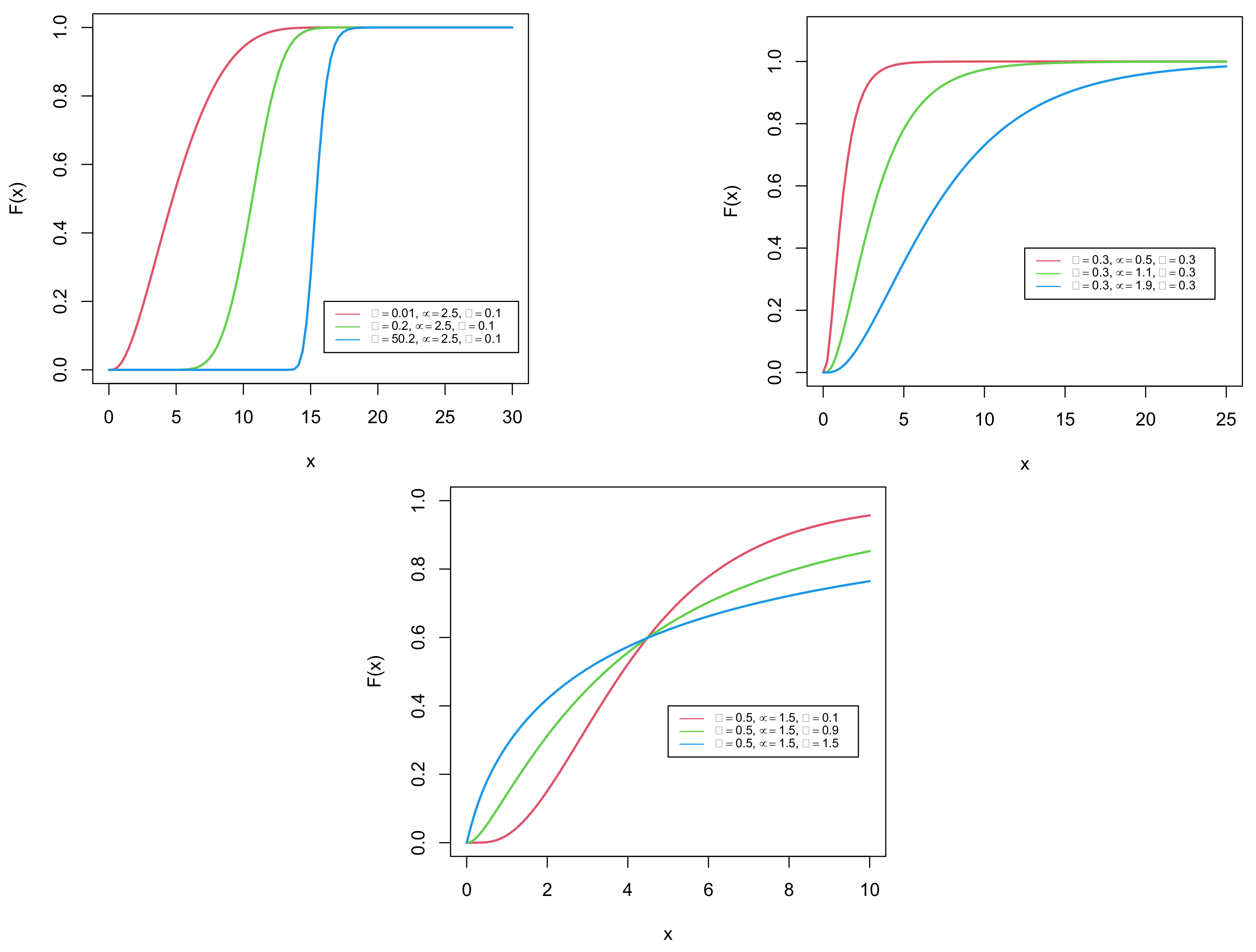
3. Definition of the Distribution

The definition of the new distribution, as well as several key features, are presented in this section. Henceforth, we call the new distribution the generalized DUS transformed log-normal (GDUSLN) distribution, and it is defined as follows:

Definition 1.

We say that a random variable X follows the GDUSLN distribution with parameters $\alpha ,\mu$ and σ if its cdf is given by

$$F\left(x\right)=\frac{\mathbf{exp}\left[{\mathsf{\Phi }}^{\alpha }\left(\frac{\log x-\mu }{\sigma }\right)\right]-1}{e-1}$$

(1)

and its pdf is given by

$$f\left(x\right)=\frac{\alpha }{\sigma x(e-1)}\varphi \left(\frac{\log x-\mu }{\sigma }\right){\mathsf{\Phi }}^{\alpha -1}\left(\frac{\log x-\mu }{\sigma }\right)\exp \left[{\mathsf{\Phi }}^{\alpha }\left(\frac{\log x-\mu }{\sigma }\right)\right],$$

(2)

where $x>0$, $\mu \in \mathbb{R}$ and $\alpha ,\sigma >0$. Furthermore, $\mathsf{\Phi }(.)$ and $\varphi (.)$ are the cdf and pdf of the standard normal distribution, respectively. It is understood that $F\left(x\right)=f\left(x\right)=0$ for $x\le 0$.

The plots in Figure 1 and Figure 2 portray the corresponding cdf and pdf of the GDUSLN distribution.

We observe that the pdf may be decreasing and unimodal with a certain flexibility in the mode and tails. It is, however, mainly right-skewed or almost symmetrical.

The cdf of the GDUSLN distribution in (1) is mitigated to the cdf of the DUS transformed log-normal (DUSLN) distribution, once $\alpha =1$. It is worth mentioning that the DUSLN distribution is not discussed in the available literature.

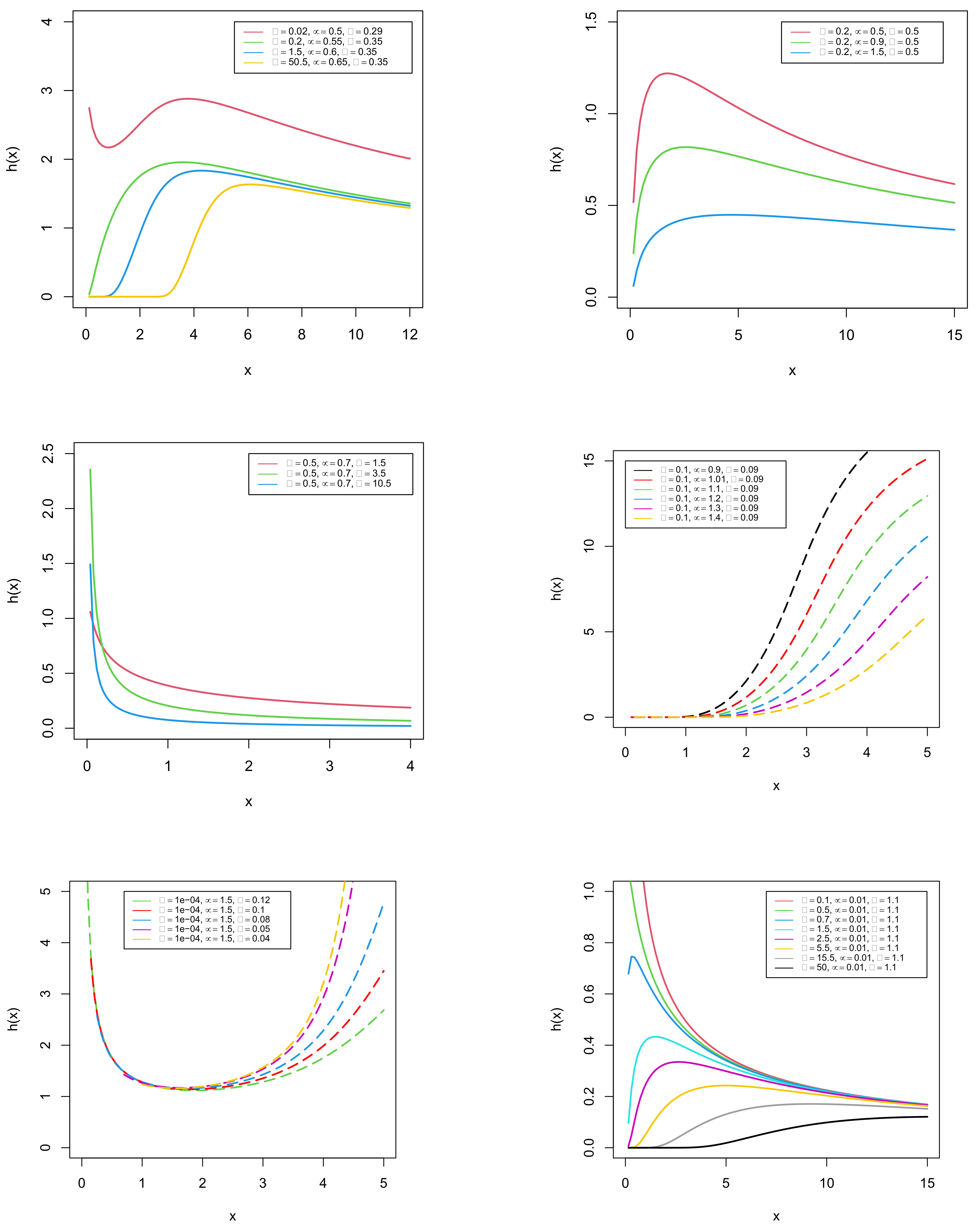
Hazard Rate Function

The hazard rate function of the GDUSLN distribution is given by

$$h\left(x\right)=\frac{f\left(x\right)}{S\left(x\right)},$$

where $S\left(x\right)=1-F\left(x\right)$ is the survival function specified by

$$S\left(x\right)=\frac{e-2-\mathbf{exp}\left[{\mathsf{\Phi }}^{\alpha }\left(\frac{\log x-\mu }{\sigma }\right)\right]}{e-1}.$$

Thus, the hazard rate function gets the form

$$h\left(x\right)=\frac{\alpha \varphi \left(\frac{\log x-\mu }{\sigma }\right){\mathsf{\Phi }}^{\alpha -1}\left(\frac{\log x-\mu }{\sigma }\right)\mathbf{exp}\left[{\mathsf{\Phi }}^{\alpha }\left(\frac{\log x-\mu }{\sigma }\right)\right]}{\sigma x\left\{e-2-\mathbf{exp}\left[{\mathsf{\Phi }}^{\alpha }\left(\frac{\log x-\mu }{\sigma }\right)\right]\right\}}.$$

Furthermore, plots in Figure 3 refer to the shapes of the hazard rate function.

It is observed that the hazard rate function possesses all the common shapes, such as increasing, decreasing, bathtub, and upside-down bathtub shapes. In this context, one of the innovative features of our model is the ability to design a bathtub-shaped failure rate function with a long flat region. This region, nevertheless, is extremely important in real-world applications, emphasizing the need for proper flat region modeling (see [11]). Furthermore, from Figure 3, it is fascinating to observe that the GDUSLN distribution has a new decreasing–increasing–decreasing shape, which we call the inverted N-shaped hazard rate function, and again possesses a special shape starting with a flat region and continuing with an increasing–decreasing shape, which we call the constant-increasing–decreasing shaped hazard rate function. More elaborately, the following results are observed from Figure 3: The hazard rate function graphs for various combinations of parameters reveal a variety of shapes including increasing ($\alpha =0.1$, $\mu \ge 0.9$, $\sigma =0.09$), decreasing ($\alpha =1.5$, $\mu =0.7$, $\sigma \ge 1.5$), bathtub ($\alpha =0.0001$, $\mu =1.5$, $0.04\le \sigma \le 0.12$), and upside-down bathtub ($\alpha =0.2$, $0.5\le \mu \le 1.5$, $\sigma =0.5$). Furthermore, it can be found that the shapes vary from decreasing to increasing via upside-down bathtub when $\alpha \ge 0.1$, $\mu =0.01$, and $\sigma =1.1$.

4. Quantile Function and Associated Measures

In this section, we derive an analytical expression for the quantile function of the GDUSLN distribution and some of its associated measures.

Theorem 1.

Let $p\in (0,1)$. If X follows the GDUSLN distribution as given in (1), then the $p^{th}$ quantile of the distribution is given by $Q_p=F^{-1}\left(p\right)$, and, more explicitly,

$$Q_p=\mathbf{exp}\left\{\mu +\sigma {\mathsf{\Phi }}^{-1}{\left[\log \left(u(e-1)+1\right)\right]}^{1/\alpha }\right\},$$

(3)

where ${\mathsf{\Phi }}^{-1}(.)$ is the quantile function of a standard normal distribution.

Proof. 

For the GDUSLN distribution, $Q_p$ is the solution of the equation

$$\begin{array}{cc}\hfill \frac{\mathbf{exp}\left[{\mathsf{\Phi }}^{\alpha }\left(\frac{\log \left(Q_p\right)-\mu }{\sigma }\right)\right]-1}{e-1}& =p,\hfill \\ \hfill \Rightarrow \mathsf{\Phi }\left(\frac{\log \left(Q_p\right)-\mu }{\sigma }\right)& ={\left\{\log \left[p(e-1)+1\right]\right\}}^{1/\alpha }.\hfill \end{array}$$

(4)

On simplifications, (4) reduces to

$$\begin{array}{c}\frac{\log \left(Q_p\right)-\mu }{\sigma }={\mathsf{\Phi }}^{-1}\left({\left\{\log \left[p(e-1)+1\right]\right\}}^{1/\alpha }\right)\hfill \\ \Rightarrow Q_p=\mathbf{exp}\left[\mu +\sigma {\mathsf{\Phi }}^{-1}\left({\left\{\log \left[p(e-1)+1\right]\right\}}^{1/\alpha }\right)\right].\hfill \end{array}$$

As a remark, since ${\mathsf{\Phi }}^{-1}(.)$ is the quantile function of a standard normal distribution, $Q_p$ in Equation (3) also gets the form

$$Q_p=\mathbf{exp}\left[\mu +\sigma \sqrt{2} {\mathrm{erf}}^{-1}\left(2{\left\{\log \left[p(e-1)+1\right]\right\}}^{1/\alpha }-1\right)\right],$$

(5)

where ${\mathrm{erf}}^{-1}(.)$ is the inverse error function.

Now, by putting $p=0.5$, in Equation (5), we get the median of the GDUSLN distribution, and it is given by

$$\mathrm{M}=Q_{0.5}=\mathbf{exp}\left[\mu +\sigma \sqrt{2} {\mathrm{erf}}^{-1}\left(2{\left\{\log \left[\frac{1}{2}(e-1)+1\right]\right\}}^{1/\alpha }-1\right)\right].$$

Equation (5) delivers the first and third quartiles of the distribution ($Q_{0.25}$ and $Q_{0.75}$) for $p=1/4$ and $p=3/4$, respectively. □

5. Estimation of Parameters

In this section, we discuss how to estimate the parameters of the GDUSLN distribution by employing two well-known methods, namely the ML and the Bayesian methods.

5.1. ML Estimation

In this subsection, we consider the ML estimation for the GDUSLN model parameters $\alpha ,\mu$ and $\sigma$. Let $X_1,X_2,\dots ,X_n$ symbolize a random sample from the GDUSLN distribution, and let $x_1,x_2,\dots ,x_n$ reflect the observed values. Then the log-likelihood function can then be written in the following form:

$$\begin{array}{cc}\hfill {\mathcal{L}}_n=& n\log \left(\alpha \right)-n\log \left(\sigma \right)-n\log (e-1)-\sum _{i=1}^n\log \left(x_i\right)+\sum _{i=1}^n\log \left[\varphi \left(\frac{\log \left(x_i\right)-\mu }{\sigma }\right)\right]\hfill \\ & +(\alpha -1)\sum _{i=1}^n\log \left[\mathsf{\Phi }\left(\frac{\log \left(x_i\right)-\mu }{\sigma }\right)\right]+\sum _{i=1}^n{\mathsf{\Phi }}^{\alpha }\left(\frac{\log \left(x_i\right)-\mu }{\sigma }\right).\hfill \end{array}$$

(6)

The score function associated with the log-likelihood function is

$$\mathbf{U}={\left(\frac{\partial {\mathcal{L}}_n}{\partial \alpha },\frac{\partial {\mathcal{L}}_n}{\partial \mu },\frac{\partial {\mathcal{L}}_n}{\partial \sigma }\right)}^T.$$

Now, the associated nonlinear log-likelihood equations are given by $\partial {\mathcal{L}}_n/\partial \alpha =0$, $\partial {\mathcal{L}}_n/\partial \mu =0$ and $\partial {\mathcal{L}}_n/\partial \sigma =0$, which can be explicated as

$$\frac{n}{\alpha }+\sum _{i=1}^n\log \left[\mathsf{\Phi }\left(\frac{\log \left(x_i\right)-\mu }{\sigma }\right)\right]+\sum _{i=1}^n{\mathsf{\Phi }}^{\alpha }\left(\frac{\log \left(x_i\right)-\mu }{\sigma }\right)\log \left[\mathsf{\Phi }\left(\frac{\log \left(x_i\right)-\mu }{\sigma }\right)\right]=0,$$

(7)

$$\begin{array}{c}\sum _{i=1}^n\frac{\log \left(x_i\right)-\mu }{{\sigma }^2}-\frac{\alpha -1}{\sigma }\sum _{i=1}^n\frac{\varphi \left(\frac{\log \left(x_i\right)-\mu }{\sigma }\right)}{\mathsf{\Phi }\left(\frac{\log \left(x_i\right)-\mu }{\sigma }\right)}\hfill \\ -\frac{\alpha }{\sigma }\sum _{i=1}^n{\mathsf{\Phi }}^{\alpha -1}\left(\frac{\log \left(x_i\right)-\mu }{\sigma }\right)\varphi \left(\frac{\log \left(x_i\right)-\mu }{\sigma }\right)=0\hfill \end{array}$$

(8)

and

$$\begin{array}{cc}\hfill -\frac{n}{\sigma }+& \sum _{i=1}^n\frac{{(\log \left(x_i\right)-\mu )}^2}{{\sigma }^3}-\frac{\alpha -1}{{\sigma }^2}\sum _{i=1}^n\left[\frac{(\log \left(x_i\right)-\mu )\varphi \left(\frac{\log \left(x_i\right)-\mu }{\sigma }\right)}{\mathsf{\Phi }\left(\frac{\log \left(x_i\right)-\mu }{\sigma }\right)}\right]\hfill \\ & -\frac{\alpha }{{\sigma }^2}\sum _{i=1}^n(\log \left(x_i\right)-\mu ){\mathsf{\Phi }}^{\alpha -1}\left(\frac{\log \left(x_i\right)-\mu }{\sigma }\right)\varphi \left(\frac{\log \left(x_i\right)-\mu }{\sigma }\right)=0,\hfill \end{array}$$

(9)

respectively.

One should get the MLEs ($\widehat{\alpha },\widehat{\mu },\widehat{\sigma }$) of the GDUSLN model parameters ($\alpha ,\mu ,\sigma$) by synergistically solving the nonlinear Equations (7)–(9).

In this paper, for the numerical optimization, we maximize the log-likelihood function for finding the MLEs. For fixing a lower and upper bound for each parameter, the numerical optimization technique “L-BFGS-B” in fitdistrplus package of the RStudio software is used. The package provides a set of functions such as fitdist and mledist for fitting univariate distributions to various types of datasets. When the log-likelihood is maximized, one should carefully choose the initial values and remove the constraints of parameters (see [12]). Fitdistrplus is a very handy package that gives unique solutions for MLEs whenever there are questions about the initial guesses and convergence of the algorithm. As a result, we use the prefit function of this package, which delivers good starting values for the algorithm. As one of the returning components of the mledist function, the indication of convergence is done by using some integer codes, such that “0” indicates successful convergence, and “1” indicates that the maximum iteration limit has been reached. As such, “10” indicates the degeneracy of the algorithm, and “100” indicates that the algorithm encountered an internal error. For more details on this package, one should go through the link “https://CRAN.R-project.org/package=fitdistrplus (accessed on 4 September 2021)”.

The asymptotic confidence intervals for the parameters $\alpha$, $\mu$ and $\sigma$ are now executed. When it comes to the second partial derivatives of ${\mathcal{L}}_n$ taken at $\widehat{\mathsf{\Theta }}=(\widehat{\alpha },\widehat{\mu },\widehat{\sigma })$, the Hessian matrix of the GDUSLN distribution can be obtained, and it is given by

$$H\left(\widehat{\mathsf{\Theta }}\right)=\left(\begin{array}{ccc}{\displaystyle \frac{{\partial }^2{\mathcal{L}}_n}{\partial {\alpha }^2}}& {\displaystyle \frac{{\partial }^2{\mathcal{L}}_n}{\partial \alpha \partial \mu }}& {\displaystyle \frac{{\partial }^2{\mathcal{L}}_n}{\partial \alpha \partial \sigma }}\\ \\ {\displaystyle \frac{{\partial }^2{\mathcal{L}}_n}{\partial \mu \partial \alpha }}& {\displaystyle \frac{{\partial }^2{\mathcal{L}}_n}{\partial {\mu }^2}}& {\displaystyle \frac{{\partial }^2{\mathcal{L}}_n}{\partial \mu \partial \sigma }}\\ \\ {\displaystyle \frac{{\partial }^2{\mathcal{L}}_n}{\partial \sigma \partial \alpha }}& {\displaystyle \frac{{\partial }^2{\mathcal{L}}_n}{\partial \sigma \partial \mu }}& {\displaystyle \frac{{\partial }^2{\mathcal{L}}_n}{\partial {\sigma }^2}}\end{array}\right).$$

Now, the observed Fisher’s information matrix $J\left(\widehat{\mathsf{\Theta }}\right)$ can be obtained by taking negative of the Hessian matrix. That is,

$$J\left(\widehat{\mathsf{\Theta }}\right)=-H\left(\widehat{\mathsf{\Theta }}\right).$$

In the case of $\alpha =1$, we derive the second partial derivatives of (6) by concerning the parameters $\mu$ and $\sigma$, and are given as follows:

$$\frac{{\partial }^2{\mathcal{L}}_n}{\partial {\mu }^2}=-\frac{1}{{\sigma }^2}\left[n+\sum _{i=1}^n\left(\frac{\log \left(x_i\right)-\mu }{\sigma }\right)\varphi \left(\frac{\log \left(x_i\right)-\mu }{\sigma }\right)\right],$$

$$\begin{array}{cc}\hfill \frac{{\partial }^2{\mathcal{L}}_n}{\partial {\sigma }^2}=\frac{n}{{\sigma }^2}-\frac{3}{{\sigma }^2}\sum _{i=1}^n{\left(\frac{\log \left(x_i\right)-\mu }{\sigma }\right)}^2& -\frac{1}{{\sigma }^2}\sum _{i=1}^n{\left(\frac{\log \left(x_i\right)-\mu }{\sigma }\right)}^3\varphi \left(\frac{\log \left(x_i\right)-\mu }{\sigma }\right)\hfill \\ & +\frac{2}{{\sigma }^2}\sum _{i=1}^n\left(\frac{\log \left(x_i\right)-\mu }{\sigma }\right)\varphi \left(\frac{\log \left(x_i\right)-\mu }{\sigma }\right)\hfill \end{array}$$

and

$$\begin{array}{cc}\hfill \frac{{\partial }^2{\mathcal{L}}_n}{\partial \mu \partial \sigma }=\frac{1}{{\sigma }^2}\sum _{i=1}^n\varphi \left(\frac{\log \left(x_i\right)-\mu }{\sigma }\right)& -\frac{2}{{\sigma }^2}\sum _{i=1}^n\left(\frac{\log \left(x_i\right)-\mu }{\sigma }\right)\hfill \\ & -\frac{1}{{\sigma }^2}\sum _{i=1}^n{\left(\frac{\log \left(x_i\right)-\mu }{\sigma }\right)}^2\varphi \left(\frac{\log \left(x_i\right)-\mu }{\sigma }\right).\hfill \end{array}$$

Clearly, $E[{\partial }^2{\mathcal{L}}_n/\partial {\mu }^2]=-n/{\sigma }^2<0$, and $E[{\partial }^2{\mathcal{L}}_n/\partial {\sigma }^2]=-2n/{\sigma }^2<0$. Hence, the information matrix is non-singular, thus following the result for the GDUSLN model also. Thus, we verified that the MLEs of the GDUSLN model parameters are unique.

Now, the inverse of the observed Fisher’s information matrix provides the variance-covariance matrix of the MLEs, which is given by

$$\mathsf{\Sigma }=J^{-1}\left(\widehat{\mathsf{\Theta }}\right)=\left(\begin{array}{ccc}{\mathsf{\Sigma }}_{11}& {\mathsf{\Sigma }}_{12}& {\mathsf{\Sigma }}_{13}\\ {\mathsf{\Sigma }}_{21}& {\mathsf{\Sigma }}_{22}& {\mathsf{\Sigma }}_{23}\\ {\mathsf{\Sigma }}_{31}& {\mathsf{\Sigma }}_{32}& {\mathsf{\Sigma }}_{33}\end{array}\right),$$

and ${\mathsf{\Sigma }}_{ij}={\mathsf{\Sigma }}_{ji}$ for $i\ne j=1,2,3$.

The asymptotically normal distribution of MLEs have been thoroughly established. That is, $\widehat{\mathsf{\Theta }}-\mathsf{\Theta }$ follows asymptotically the multivariate normal distribution $N_3(0,\mathsf{\Sigma })$.

Using the following formulae, we calculate the $100\times (1-\delta )\%$ asymptotic confidence intervals for parameters.

$$\alpha \in \left\{\widehat{\alpha }\mp Z_{\delta /2}\sqrt{{\mathsf{\Sigma }}_{11}}\right\},\mu \in \left\{\widehat{\mu }\mp Z_{\delta /2}\sqrt{{\mathsf{\Sigma }}_{22}}\right\}\mathrm{and}\sigma \in \left\{\widehat{\sigma }\mp Z_{\delta /2}\sqrt{{\mathsf{\Sigma }}_{33}}\right\},$$

where $Z_{\delta }$ is the upper ${\delta }^{\mathrm{th}}$ percentile of the standard normal distribution.

5.2. Bayesian Estimation

In this subsection, we perform the Bayesian analysis for the GDUSLN model parameters. To do so, each parameter should have a prior density. We employ two types of priors for this: the half-Cauchy ($HC$) and the normal (N) priors. The pdf of the HC distribution with scale parameter a is defined as

$$f_{HC}\left(x_{*}\right)=\frac{2a}{\pi (x_{*}^2+a^2)},x_{*}>0,a>0.$$

(10)

The HC distribution has no mean nor variance. Meanwhile, its mode is equal to 0. Since the pdf of the HC is virtually flat but not totally flat at scale value equals 25, which verges on acquiring adequate information for the numerical approximation algorithm to continue looking at the target posterior pdf, the HC distribution with $a=25$ is recommended as a noninformative prior. Ref. [13] suggested that the uniform distribution, or whether more information is required, is a superior alternative to the HC distribution. As a result, for the parameters $\alpha$ and $\sigma$, the HC distribution with $a=25$ is chosen as a noninformative prior distribution in this article. Thus, we set the prior distributions of the parameters to be

$$\begin{array}{c}\mu \sim N(0,1000)\hfill \\ \alpha ,\sigma \sim HC\left(25\right).\hfill \end{array}$$

(11)

The log-likelihood function of the GDUSLN distribution is given in Equation (6). Now, using (6) and (11), we obtain the joint posterior pdf as given by

$$\pi (\mu ,\alpha ,\sigma |x)\propto {\mathcal{L}}_n\times \pi \left(\mu \right)\times \pi \left(\alpha \right)\times \pi \left(\sigma \right).$$

(12)

From (12), it is obvious that there is no analytical solution to find out the Bayesian estimates. Thus, we use a remarkable method of simulation, namely the Metropolis-Hastings algorithm of the Markov Chain Monte Carlo (MCMC) method.

6. Bootstrap Confidence Intervals

In this section, we use the parametric bootstrap method to approximate the distribution of MLEs of the GDUSLN model parameters. Then, we can use the bootstrap distribution to estimate confidence intervals of each parameter for the fitted GDUSLN distribution. Let $\widehat{\mathsf{\Theta }}$ be a MLE on the set of parameters of interest $\mathsf{\Theta }=(\alpha ,\mu ,\sigma )$ using a given dataset $\{x_1,x_2,\dots ,x_n\}$. The bootstrap is a method to estimate the distribution of statistic $\widehat{\mathsf{\Theta }}$ by getting a random sample ${\mathsf{\Theta }}_1^{*},{\mathsf{\Theta }}_2^{*},\dots ,{\mathsf{\Theta }}_B^{*}$ for $\mathsf{\Theta }$ based on B random samples that are drawn with replacement from $\{x_1,x_2,\dots ,x_n\}$, see [14]. The bootstrap sample ${\mathsf{\Theta }}_1^{*},{\mathsf{\Theta }}_2^{*},\dots ,{\mathsf{\Theta }}_B^{*}$ can be used to construct bootstrap confidence intervals for the parametric set $\mathsf{\Theta }=(\alpha ,\mu ,\sigma )$ of the GDUSLN distribution.

Thus, using the following formulae, we calculate the $100\times (1-\delta )\%$ bootstrap confidence intervals for parameters:

$$\alpha \in \left\{\widehat{\alpha }\mp z_{\delta /2}{\widehat{se}}_{\alpha ,boot}\right\},\mu \in \left\{\widehat{\mu }\mp z_{\delta /2}{\widehat{se}}_{\mu ,boot}\right\},\sigma \in \left\{\widehat{\sigma }\mp z_{\delta /2}{\widehat{se}}_{\sigma ,boot}\right\},$$

where $z_{\delta }$ denotes the ${\delta }^{\mathrm{th}}$ percentile of the bootstrap sample and, for $\theta \in \{\alpha ,\mu ,\sigma \}$,

$${\widehat{se}}_{\theta ,boot}=\sqrt{\frac{1}{B}\sum _{b=1}^B{\left({\theta }_b^{*}-\frac{1}{B}\sum _{b=1}^B{\theta }_b^{*}\right)}^2}.$$

7. GDUSLN Regression Model

In this section, we define a regression model based on the GDUSLN distribution called the GDUSLN regression model. For finding the model based on the GDUSLN distribution, we consider a random variable X following the GDUSLN distribution with pdf as given in (2) and we define another random variable Y as $Y=\log \left(X\right)$. Then the Y has the following pdf:

$$f_Y\left(y\right)=\frac{\alpha }{\sigma (e-1)}\varphi \left(\frac{y-\mu }{\sigma }\right){\mathsf{\Phi }}^{\alpha -1}\left(\frac{y-\mu }{\sigma }\right)\mathbf{exp}\left[{\mathsf{\Phi }}^{\alpha }\left(\frac{y-\mu }{\sigma }\right)\right],$$

(13)

where $y\in \mathbb{R}$, the shape parameter $\alpha >0$, the location parameter $\mu \in \mathbb{R}$, and the scale parameter $\sigma >0$. We allude to Equation (13) as the Log-GDUSLN (Log GDUS log-normal) distribution or otherwise, GDUS normal (GDUSN) distribution. It is worth mentioning that the GDUSN distribution is not covered in any of the existing literature. In this setting, the standardized random variable $Z=(Y-\mu )/\sigma$ has the pdf given by

$$f_Z\left(z\right)=\frac{\alpha }{e-1}\varphi \left(z\right){\mathsf{\Phi }}^{\alpha -1}\left(z\right)\mathbf{exp}\left[{\mathsf{\Phi }}^{\alpha }\left(z\right)\right].$$

(14)

Now, the linear location-scale regression model by linking the response variable, say $y_i$, and the explanatory variable vector, say ${\mathrm{v}}_i^T=(v_{i1},v_{i2},\dots ,v_{ip})$, is obtained as:

$$y_i={\mu }_i+\sigma z_i,i=1,2,\dots ,n,$$

(15)

where $z_i$ is the random error component, has the pdf as given in (14), ${\mu }_i={\mathrm{v}}_i^T\tau$ is the location parameter of $y_i$, where $\tau ={({\tau }_1,{\tau }_2,\dots ,{\tau }_p)}^T$, $\alpha$ and $\sigma$ are unknown parameters. The linear model $\mu =V\tau$ represents the location parameter vector $\mu ={({\mu }_1,{\mu }_2,\dots ,{\mu }_n)}^T$, where $V={(V_1,V_2,\dots ,V_n)}^T$ is a known model matrix.

Ultimately, in this article, we propose the GDUSLN regression model from (15) and it is given by

$$x_i=\mathbf{exp}\left(y_i\right)=\mathbf{exp}({\mu }_i+\sigma z_i),i=1,2,\dots ,n.$$

(16)

Consider a sample $(x_1,{\mathrm{v}}_1),(x_2,{\mathrm{v}}_2),\dots ,(x_n,{\mathrm{v}}_n)$ of n independent observations. Here, typical likelihood estimation approach can be used. Now, for the vector of parameters $\mathbf{\psi }={({\tau }^T,\alpha ,\sigma )}^T$ from model (16), the total log-likelihood function for right censored has the form

$$\begin{array}{cc}\hfill l\left(\mathbf{\psi }\right)=& \log \left\{\prod _{i=1}^n{\left[f\left(x_i\right)\right]}^{{\delta }_i}{\left[S\left(x_i\right)\right]}^{1-{\delta }_i}\right\}\hfill \\ \hfill =& \sum _{i=1}^n{\delta }_i\log \left[f\left(x_i\right)\right]+\sum _{i=1}^n(1-{\delta }_i)\log \left[S\left(x_i\right)\right],\hfill \end{array}$$

with ${\delta }_i=1$ if survival (uncensored) and ${\delta }_i=0$, if not (censored). Furthermore, for $i=1,2,\dots ,n$, $f\left(x_i\right)$ and $S\left(x_i\right)$ are the pdf and survival function of the GDUSLN distribution taken at $x_i$, respectively.

8. Bayesian Regression Model

The Bayesian technique is shown to be particularly effective in analyzing survival models in many practical circumstances. Ergo, in this section, we will look at how the Bayesian approach fits the regression model based on the GDUSLN distribution when prior pieces of information about the parameters are taken into account. Accordingly, for the purpose of Bayesian analysis of this model, we implemented a simulation method.

Now, to perform a Bayesian analysis, one should adopt prior distributions for the parameters. Here, similar to Section 5.2, we utilized two different prior distributions, the HC and N priors. The pdf of the HC distribution with a as the scale parameter is given in Equation (10). Now, we write the right censored likelihood function as

$$L=\prod _{i=1}^n{\left[f\left(x_i\right)\right]}^{{\delta }_i}{\left[S\left(x_i\right)\right]}^{1-{\delta }_i},$$

(17)

with ${\delta }_i=1$, if survival (uncensored) and ${\delta }_i=0$, if not (censored). Furthermore, for $i=1,2,\dots ,n$, $f\left(x_i\right)$ and $S\left(x_i\right)$ are the pdf and survival function of the GDUSLN distribution taken at $x_i$, respectively. We use the link function specified by

$$\mu =V\tau$$

(18)

as a linear combination of explanatory variables. Thus, we set the prior distributions of the parameters to be

$$\begin{array}{c}{\tau }_j\sim N(0,1000);j=1,2,\dots ,J\hfill \\ \alpha ,\sigma \sim HC\left(25\right).\hfill \end{array}$$

(19)

Now, using (17)–(19), the joint posterior pdf is obtained as

$$\pi (\tau ,\alpha ,\sigma |x,V)\propto L(x|V,\tau ,\alpha ,\sigma )\times \pi \left(\tau \right)\times \pi \left(\alpha \right)\times \pi \left(\sigma \right).$$

(20)

From Equation (20), it is clear that the analytical solution is not possible to find out the Bayesian estimates. Thus, similar to Section 5.2, we use the method of simulation, namely, the Metropolis–Hastings algorithm of the MCMC method.

9. Performance of the Estimates Using Simulation Study

In this section, we conduct simulation experiments to assess the long-run performances of ML and Bayesian estimates of the GDUSLN distribution parameters for some finite sample sizes. We have generated samples of sizes $n=50,100,250,500,750$, and 1000 from the GDUSLN distribution using various values of parameters.

9.1. Simulation Study for the MLE

Here, the iteration is conducted 1001 times. Thus, we computed the average of the biases, mean squared errors (MSEs), coverage probabilities (CPs), and average lengths (ALs) of each parameter estimate for all replications in the respective sample sizes.

The analysis computes the values for the average biases and MSEs of the simulated estimates by the following formulae:

• Average bias = ${\displaystyle \frac{1}{1001}}{\displaystyle \sum _{i=1}^{1001}}({\widehat{\theta }}_i-\theta )$, and
• Average MSE = ${\displaystyle \frac{1}{1001}}{\displaystyle \sum _{i=1}^{1001}}{({\widehat{\theta }}_i-\theta )}^2$,

where i is the number of iterations, and $\theta \in \{\alpha ,\mu ,\sigma \}$ and $\widehat{\theta }$ is the estimate of $\theta$. The results of each parameter set are reported in

Table 1. The MLE simulation results for ($\alpha =0.01$, $\mu =0$, $\sigma =1$).

Parameters	n	MLE	Bias	MSE	CP	AL
$\alpha$	50	0.0265	0.0165	0.0117	0.9860	0.1884
	100	0.0171	0.0071	0.0029	0.9900	0.0703
	250	0.0128	0.0028	0.000062	0.9980	0.0285
	500	0.0118	0.0018	0.000025	0.9999	0.0170
	750	0.0118	0.0018	0.000011	0.9999	0.0138
	1000	0.0117	0.0017	$8.722\times {10}^{-6}$	0.9999	0.0118
$\mu$	50	−0.2877	−0.2877	2.0349	0.9999	6.5780
	100	−0.1107	−0.1107	0.8001	0.9990	3.9497
	250	−0.0636	−0.0636	0.1924	0.9980	2.2907
	500	−0.0306	−0.0306	0.0821	0.9910	1.5273
	750	−0.0809	−0.0809	0.0398	0.9880	1.2473
	1000	−0.0774	−0.0774	0.0310	0.9860	1.0726
$\sigma$	50	1.2084	0.2084	0.4160	0.9880	3.0793
	100	1.1361	0.1361	0.1808	0.9910	1.8328
	250	1.0964	0.0964	0.0519	0.9950	1.0693
	500	1.0685	0.0685	0.0238	0.9970	0.7011
	750	1.0737	0.0737	0.0160	0.9950	0.5817
	1000	1.0699	0.0699	0.0131	0.9950	0.4989

,

Table 2. The MLE simulation results for ($\alpha =1.5$, $\mu =0$, $\sigma =1$).

Parameters	n	MLE	Bias	MSE	CP	AL
$\alpha$	50	3.4450	1.9450	17.9693	0.8212	29.7384
	100	2.8944	1.3944	11.9153	0.8352	17.3465
	250	2.3789	0.8789	7.2803	0.8851	9.2240
	500	1.8799	0.3799	2.2217	0.8981	4.5803
	750	1.7522	0.2522	0.7747	0.9341	3.3028
	1000	1.6936	0.1936	0.5628	0.9281	2.7298
$\mu$	50	−0.1516	−0.1516	1.5050	0.9211	6.7687
	100	−0.1322	−0.1322	1.0738	0.9221	4.7298
	250	−0.1360	−0.1360	0.6004	0.9471	3.0166
	500	−0.0557	−0.0557	0.3029	0.9461	2.0178
	750	−0.0638	−0.0638	0.1646	0.9610	1.6335
	1000	−0.0495	−0.0495	0.1298	0.9491	1.4036
$\sigma$	50	0.9850	−0.0151	0.1354	0.9351	1.9180
	100	0.9993	−0.00076	0.0946	0.9261	1.3519
	250	1.0217	0.0217	0.0486	0.9590	0.8666
	500	1.0080	0.0080	0.0253	0.9421	0.5928
	750	1.0136	0.0136	0.0139	0.9640	0.4816
	1000	1.0110	0.0110	0.0112	0.9511	0.4152

,

Table 3. The MLE simulation results for ($\alpha =3.5$, $\mu =0$, $\sigma =1$).

Parameters	n	MLE	Bias	MSE	CP	AL
$\alpha$	50	3.3691	−0.1309	7.3639	0.7602	26.7792
	100	3.7652	0.2652	6.7212	0.8092	20.8407
	250	4.0625	0.5625	5.5040	0.8681	14.4071
	500	3.9641	0.4641	4.1423	0.8931	10.1917
	750	4.0522	0.5523	3.3380	0.9271	8.6438
	1000	3.8094	0.3094	2.5673	0.9261	6.9700
$\mu$	50	0.3772	0.3772	0.9082	0.8841	5.7295
	100	0.1891	0.1891	0.5807	0.9081	4.2434
	250	0.0229	0.0229	0.3165	0.9431	2.8635
	500	−0.00075	−0.00075	0.2164	0.9461	2.0896
	750	−0.0493	−0.0493	0.1510	0.9650	1.7545
	1000	−0.0105	−0.0105	0.1240	0.9610	1.5016
$\sigma$	50	0.8607	−0.1393	0.0962	0.9051	1.5967
	100	0.9266	−0.0734	0.0551	0.9211	1.1520
	250	0.9831	−0.0169	0.0250	0.9560	0.7596
	500	0.9943	−0.0057	0.0160	0.9541	0.5523
	750	1.0085	0.0085	0.0106	0.9750	0.4605
	1000	0.9992	−0.00078	0.0089	0.9630	0.3970

and

Table 4. The MLE simulation results for ($\alpha =0.01$, $\mu =1.5$, $\sigma =0.5$).

Parameters	n	MLE	Bias	MSE	CP	AL
$\alpha$	50	0.8120	0.8020	99.3306	0.9990	17.2775
	100	0.0597	0.0497	0.0180	0.9960	0.3258
	250	0.0278	0.01780	0.0009	0.9950	0.0855
	500	0.0120	0.010	0.00023	0.9970	0.0393
	750	0.0172	0.0072	0.00012	0.9990	0.0260
	1000	0.0160	0.0060	$7.792\times {10}^{-5}$	0.9970	0.0201
$\mu$	50	−0.5673	−2.0673	10.6468	0.9950	9.7789
	100	0.6150	−0.8850	1.6948	0.9920	4.0846
	250	1.0235	−0.4765	0.4590	0.9690	1.9015
	500	1.1998	−0.3002	0.1834	0.9421	1.1122
	750	1.2758	−0.2242	0.1068	0.9091	0.8285
	1000	1.3111	−0.1889	0.0784	0.8711	0.6806
$\sigma$	50	1.3170	0.8170	1.3831	0.9980	3.7459
	100	0.9005	0.4005	0.3222	0.9880	1.8729
	250	0.7345	0.2344	0.1043	0.9860	0.9233
	500	0.6570	0.1570	0.0474	0.9600	0.5459
	750	0.6234	0.1234	0.0293	0.9481	0.4065
	1000	0.6059	0.1059	0.0219	0.9031	0.3325

.

It can be observed that with the increase in sample size, the MSEs and the ALs corresponding to each estimate fall. Furthermore, the CPs of the confidence intervals for each parameter are fairly close to the $95\%$ nominal levels. This confirms the consistent performance of MLEs of the GDUSLN distribution.

9.2. Simulation Study for Bayesian Estimates

We consider the prior distributions for the GDUSLN parameters as given in Section 5.2. Hence, here we iterated each sample 10,001 times. For each parameter set of respective sample sizes, the posterior summary results such as mean, standard deviation (SD), Monte Carlo error (MCE), $95\%$ confidence interval (CI), and median are presented in

Table 5. Posterior summary results for ($\alpha =0.01$, $\mu =0$, $\sigma =1$).

Parameters	n	Mean	SD	MCE	95% CI	Median
$\alpha$	50	0.1442	0.1824	0.0519	(0.0042, 0.6596)	0.0570
	100	0.0334	0.1207	0.0132	(0.0063, 0.0611)	0.0167
	250	0.0220	0.0212	0.0081	(0.0141, 0.0898)	0.0150
	500	0.0185	0.0076	0.0024	(0.0118, 0.0466)	0.0172
	750	0.0231	0.0052	0.0011	(0.0208, 0.0262)	0.0208
	1000	0.0149	0.0009	0.00058	(0.0135, 0.0156)	0.0154
$\mu$	50	−3.4733	3.0723	0.8754	(−9.6826, 0.8414)	−2.7271
	100	−0.3452	1.2663	0.5454	(−2.4443, 1.5253)	−0.1428
	250	−0.4035	0.5696	0.2240	(−2.3547, −0.0708)	−0.1831
	500	−0.5347	0.4115	0.1992	(−0.8684, 0.8708)	−0.6868
	750	−0.7501	0.4026	0.1564	(−1.2204, 0.1082)	−0.6910
	1000	−0.7085	0.3481	0.1240	(−0.8361, 0.6058)	−0.8361
$\sigma$	50	2.3915	1.2560	0.3398	(0.6745, 5.0700)	2.1073
	100	1.3575	0.8723	0.2097	(0.7271, 2.4231)	1.1131
	250	1.3106	0.5267	0.1905	(1.1652, 2.6330)	1.1652
	500	1.2938	0.2787	0.0835	(1.0247, 2.0993)	1.2751
	750	1.4881	0.2525	0.0783	(1.4131, 1.7219)	1.4131
	1000	1.1867	0.0506	0.03160	(1.1108, 1.2723)	1.2102

,

Table 6. Posterior summary results for ($\alpha =1.5$, $\mu =0$, $\sigma =1$).

Parameters	n	Mean	SD	MCE	95% CI	Median
$\alpha$	50	4.1662	7.3244	2.0432	(0.0093, 20.6094)	0.9974
	100	4.2131	5.2494	1.5542	(0.0717, 22.7491)	2.2271
	250	2.2417	2.1410	0.6711	(0.0846, 9.0499)	1.6914
	500	1.5378	1.6005	0.2416	(0.4581, 4.3854)	1.3377
	750	1.6211	0.4696	0.1316	(0.7095, 2.7769)	1.5799
	1000	1.4906	0.2316	0.0615	(1.4512, 2.0980)	1.4514
$\mu$	50	0.0369	1.2995	0.3834	(−2.5848, 2.0525)	0.3404
	100	−0.4092	1.0441	0.3193	(−2.6677, 1.8552)	−0.1807
	250	0.1550	0.7931	0.2581	(−1.3816, 1.7138)	0.0570
	500	0.1253	0.4695	0.0839	(−1.0430, 0.9718)	0.1231
	750	−0.1065	0.2889	0.0811	(−0.7150, 0.5232)	−0.0650
	1000	−0.0170	0.1420	0.0331	(−0.4267, 0.0236)	0.0226
$\sigma$	50	0.8448	0.3702	0.1073	(0.1403, 1.5976)	0.8392
	100	1.0815	0.2833	0.0866	(0.3392, 1.5447)	1.0771
	250	0.8506	0.2329	0.0747	(0.3265, 1.2604)	0.8995
	500	0.9565	0.1442	0.0291	(0.6713, 1.2297)	0.9641
	750	1.0589	0.0986	0.0277	(0.8357, 1.2506)	1.0656
	1000	1.0097	0.0521	0.0142	(0.9907, 1.1366)	0.9907

,

Table 7. Posterior summary results for ($\alpha =3.5$, $\mu =0$, $\sigma =1$).

Parameters	n	Mean	SD	MCE	95% CI	Median
$\alpha$	50	8.4499	7.6768	2.1079	(0.1380, 24.5375)	6.2095
	100	5.3500	9.4171	1.7008	(0.3285, 13.5378)	3.2753
	250	2.3796	2.7053	0.8287	(0.3081, 10.1427)	1.3011
	500	2.8784	2.2901	0.8092	(1.0101, 10.4748)	1.9153
	750	4.4209	2.0585	0.6653	(2.6587, 6.5986)	4.0738
	1000	2.8436	1.4592	0.3074	(1.6108, 6.7540)	2.8355
$\mu$	50	0.2228	0.9573	0.2940	(−1.0484, 2.0049)	−0.0019
	100	0.0332	0.7769	0.2336	(−1.3759, 1.4283)	0.0934
	250	0.5618	0.6370	0.1979	(−0.7925, 1.4505)	0.6533
	500	0.2950	0.4991	0.1552	(−0.8614, 0.9619)	0.4101
	750	−0.1969	0.4249	0.1302	(−0.7398, 0.2054)	−0.1912
	1000	0.2197	0.3472	0.1082	(−0.6779, 0.5688)	0.1770
$\sigma$	50	0.8080	0.2633	0.0797	(0.2915, 1.1814)	0.9090
	100	0.8718	0.2162	0.0649	(0.4689, 1.1968)	0.8866
	250	0.7443	0.1800	0.0582	(0.4790, 1.0736)	0.7109
	500	0.9343	0.1354	0.0390	(0.7414, 1.2237)	0.9326
	750	1.0692	0.1295	0.0371	(0.9619, 1.2253)	1.0566
	1000	0.9466	0.1004	0.0306	(0.8628, 1.2225)	0.9323

and

Table 8. Posterior summary results for ($\alpha =0.01$, $\mu =1.5$, $\sigma =0.5$).

Parameters	n	Mean	SD	MCE	95% CI	Median
$\alpha$	50	0.1779	0.2908	0.0794	(0.0041, 1.3728)	0.0583
	100	0.0734	0.0987	0.0260	(0.0060, 0.3889)	0.0330
	250	0.0300	0.0488	0.0124	(0.0075, 0.1611)	0.0160
	500	0.0160	0.0364	0.0062	(0.0110, 0.0843)	0.0110
	750	0.0159	0.0090	0.0021	(0.0061, 0.0240)	0.0147
	1000	0.0092	0.0069	0.0012	(0.0068, 0.0202)	0.0076
$\mu$	50	−0.1424	1.4196	0.3924	(−4.0866, 1.5825)	0.3360
	100	0.6450	0.9748	0.2626	(−1.6869, 1.8166)	0.9622
	250	0.9545	0.6301	0.1960	(−0.9009, 1.4706)	1.1956
	500	1.1691	0.3183	0.0822	(−0.1112, 1.2343)	1.2343
	750	1.3269	0.2115	0.0573	(1.0271, 1.7025)	1.3379
	1000	1.6181	0.1493	0.0226	(1.2482, 1.7385)	1.6251
$\sigma$	50	0.9612	0.5966	0.1678	(0.2695, 2.6994)	0.8186
	100	0.9495	0.5012	0.1325	(0.3651, 2.0675)	0.8613
	250	0.6918	0.3148	0.0984	(0.4297, 1.5184)	0.6134
	500	0.5719	0.1891	0.0508	(0.5299, 1.4506)	0.5300
	750	0.5760	0.1087	0.0281	(0.3929, 0.7253)	0.5727
	1000	0.4504	0.1012	0.0194	(0.4045, 0.7358)	0.4185

.

It is observed that the SD and MCE decrease as the sample size increases, which predicts the consistency of Bayesian estimates of the GDUSLN distribution.

10. Applications and Empirical Study

This section is comprised of demonstrating the empirical importance of the GDUSLN distribution. We consider two real datasets from the area of biological science. One is the univariate cancer survival dataset, which is used to compare the data modeling ability of the GDUSLN distribution over some competitive distributions, and the other is the heart transplant dataset for the regression study. We use the RStudio software for numerical evaluations of these datasets.

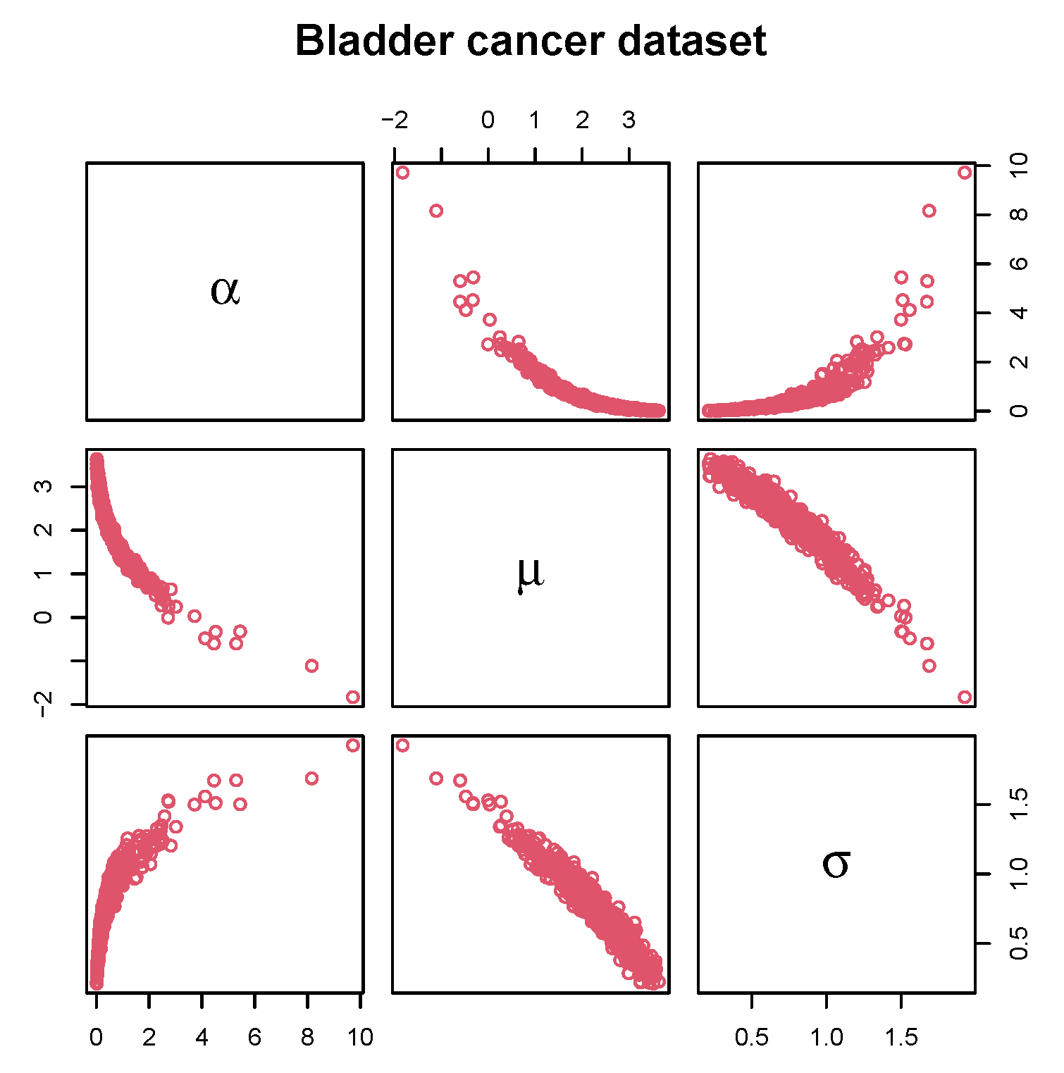
10.1. Cancer Survival Data

First, we utilize the dataset from [15] as a biological dataset, which represents an uncensored univariate dataset comprised of the remission times (in months) of a random sample of 128 bladder cancer patients. The descriptive measures of the real dataset, which include sample size (n), minimum ($min$), first quartile ($Q_1$), median ($Md$), third quartile ($Q_3$), maximum ($max$), and inter-quartile range (IQR) are given in

Table 9. Descriptive statistics of real dataset.

Statistic	n	$min$	$Q_1$	$Md$	$Q_3$	$max$	IQR
Values	128	0.08	3.348	6.280	11.678	79.05	8.330

.

We also investigate the empirical hazard rate function for the biology dataset using the idea of a total time on test (TTT) plot. The TTT plot is a graph being used to distinguish between several types of aging as displayed in the hazard rate shapes. The common shapes of the hazard rate possess constant, increasing, decreasing, bathtub, and upside-down bathtub shapes, and can be identified by using the TTT plot by the following methods:

• A plot around the diagonal indicates a constant hazard rate, that is, the failure times can be considered exponentially distributed.
• A concave plot (above the diagonal) indicates an increasing hazard rate function.
• A convex plot (under the diagonal) indicates a decreasing hazard rate function.
• A plot which first is convex, and then concave indicates a bathtub shaped hazard rate function.
• A plot which first is concave, and then convex indicates an upside-down bathtub shaped hazard rate function.

For more about the TTT plot, see details in [16]. The TTT plot is drawn by plotting

$$T\left(\frac{i}{n}\right)=\frac{{\displaystyle \sum _{r=1}^i}{x}_{r:n}+(n-i)x_{i:n}}{{\displaystyle \sum _{r=1}^n}{x}_{r:n}}$$

against $i/n$, where $i=1,2,\dots ,n$ and $x_{r:n}$, $r=1,2,\dots ,n$ are the order statistics of the sample.

Thus, the plot in Figure 4 indicates that this dataset represents an upside-down bathtub shaped hazard rate function. This case is covered by the characteristics of the GDUSLN distribution.

To show the potential advantage of the GDUSLN distribution, the following distributions are considered for comparison:

• The two-parameter LN distribution.
• The exponentiated LN (ELN) distribution or otherwise, the log-power-normal distribution (see [17]) with pdf

  $$f\left(x\right)=\frac{\alpha }{x\sigma }\varphi \left(\frac{\log x-\mu }{\sigma }\right){\left[\mathsf{\Phi }\left(\frac{\log x-\mu }{\sigma }\right)\right]}^{\alpha -1},x>0,\mu \in \mathbb{R},\alpha ,\sigma >0.$$
• Generalized half-normal (GHN) distribution (see [18]) with pdf

  $$f\left(x\right)=\sqrt{\frac{2}{\pi }}\left(\frac{\alpha }{x}\right){\left(\frac{x}{\sigma }\right)}^{\alpha }\mathbf{exp}\left\{-\frac{1}{2}{\left(\frac{x}{\sigma }\right)}^{2\alpha }\right\},x,\alpha ,\sigma >0.$$
• The new generalized Lindley distribution (NGLD) (see [19]) with pdf

  $$f\left(x\right)=\frac{e^{-\mu x}}{1+\mu }\left(\frac{{\mu }^{\alpha +1}{x}^{\alpha -1}}{\mathsf{\Gamma }\left(\alpha \right)}+\frac{{\mu }^{\sigma }{x}^{\sigma -1}}{\mathsf{\Gamma }\left(\sigma \right)}\right),x>0,\alpha ,\mu ,\sigma >0,$$

  where $\mathsf{\Gamma }\left(p\right)={\int }_0^{\infty }{t}^{p-1}{e}^{-t}dt$.
• The modified Weibull (MoW) distribution (see [20]) with pdf

  $$f\left(x\right)=\mu \sigma {\left(\frac{x}{\alpha }\right)}^{\mu -1}\mathbf{exp}\left[{\left(\frac{x}{\alpha }\right)}^{\mu }+\alpha \sigma \left(1-e^{{(x/\alpha )}^{\mu }}\right)\right],x>0,\alpha ,\mu ,\sigma >0.$$
• The Weibull distribution with pdf

  $$f\left(x\right)=\frac{\alpha }{\sigma }{\left(\frac{x}{\sigma }\right)}^{\alpha -1}{e}^{-{(x/\sigma )}^{\alpha }},x>0,\alpha ,\sigma >0.$$

We compare the competitive models to the proposed models using the following statistical tools: negative log-likelihood ($-\log L$), Kolmogorov–Smirnov (KS), Cramér-von Misses ($W^{*}$), Anderson–Darling ($A^{*}$) statistics, Akaike Information Criterion (AIC), and Bayesian Information Criterion (BIC) values.

Table 10. Bladder cancer dataset: MLEs of the parameters.

Distribution	MLE
GDUSLN($\alpha ,\mu ,\sigma$)	$\widehat{\alpha }$ = 0.2330, $\widehat{\mu }$ = 2.5675, $\widehat{\sigma }$ = 0.6660
LN($\mu ,\sigma$) ine ELN($\alpha ,\mu ,\sigma$)	$\widehat{\mu }$ = 1.7423, $\widehat{\sigma }$ = 1.0647 $\widehat{\alpha }$ = 0.1514, $\widehat{\mu }$ = 3.0502, $\widehat{\sigma }$ = 0.5401
GHN($\mu ,\sigma$)	$\widehat{\mu }$ = 0.7593, $\widehat{\sigma }$ = 11.4510
NGLD($\alpha ,\mu ,\sigma$)	$\widehat{\alpha }$ = 1.1848, $\widehat{\mu }$ = 0.1287, $\widehat{\sigma }$ = 1.1851
MoW($\alpha ,\mu ,\sigma$)	$\widehat{\alpha }$ = $4.565\times {10}^{-6}$, $\widehat{\mu }$ = 0.1378, $\widehat{\sigma }$ = 123.976
Weibull($\alpha ,\sigma$)	$\widehat{\alpha }$ = 1.0546, $\widehat{\sigma }$ = 9.4371

and

Table 11. Bladder cancer dataset: GOF statistics results.

Distribution	$-\log L$	AIC	BIC	KS	$W^{*}$	$A^{*}$
GDUSLN	409.0979	824.1958	832.7519	0.0551	0.0646	0.4318
LN	412.6565	829.3131	835.0171	0.0644	0.1313	0.8708
ELN	410.0441	826.0883	834.6444	0.0562	0.0846	0.5590
GHN	418.7864	841.5727	847.2768	0.1018	0.3815	2.4201
NGLD	411.0846	828.1691	836.7252	0.0751	0.1415	0.8233
MoW	419.3804	844.7608	853.3169	0.0949	0.3632	2.3184
Weibull	411.8936	827.7873	833.4913	0.0731	0.1670	1.0441

display the corresponding MLEs and goodness-of-fit (GOF) statistics of the considered distributions corresponding to the bladder cancer dataset.

From these tables, we see that the GOF statistics values of the GDUSLN distribution are smaller than those of the other compared distributions. It can also be noted that the optimization algorithm possesses successful convergence as indicated in Section 5.1.

The empirical cdf and quantile-quantile (Q-Q) plots for the real dataset are given in Figure 5.

This figure shows some nice-shaped curves for those empirical and fitted functions. Thus, we conclude that the GDUSLN distribution is the most suitable distribution for this dataset compared to that of the other distributions.

Now, the Hessian matrix corresponding to bladder cancer dataset is obtained as

$$H\left(\mathsf{\Theta }\right)=\left(\begin{array}{ccc}1918.1947& 407.3235& -825.5481\\ 407.3235& 126.7731& -77.560\\ -825.5481& -77.560& 620.8239\end{array}\right),$$

and the corresponding estimated variance-covariance matrix is

$$\mathsf{\Sigma }=\left(\begin{array}{ccc}0.0332& -0.0863& 0.0334\\ -0.0863& 0.2326& -0.0856\\ 0.0334& -0.0856& 0.0353\end{array}\right).$$

It is observed that the determinant value of the observed information matrix ($|J(\widehat{\mathsf{\Theta }})|$) is non-zero, and hence satisfies the non-singularity condition of the information matrix. Now,

Table 12. The 95% asymptotic confidence intervals of the GDUSLN parameters based on bladder cancer dataset.

Parameter	Lower	Upper
$\alpha$	−0.1241	0.5901
$\mu$	1.6222	3.5128
$\sigma$	0.2978	1.0341

provides the 95 percent asymptotic confidence intervals for the GDUSLN parameters.

Next, we focus on estimating the parameters of the GDUSLN distribution using the Bayesian procedure based on the above discussed univariate bladder cancer survival dataset. In the context of Bayesian estimation, the analysis was performed using the Metropolis–Hastings algorithm of the MCMC method with 1000 iterations. For comparing Bayes estimates with the MLEs, both the estimates of the GDUSLN parameters for the real dataset are given in

Table 13. MLEs and Bayes estimates of the GDUSLN parameters on bladder cancer dataset.

Parameter	ML	Bayes
$\alpha$	0.2330	0.2058
$\mu$	2.5675	2.6519
$\sigma$	0.6660	0.6395

. The numerical computations on Bayesian estimation are done using RStudio software.

10.1.1. Results on Bootstrap Confidence Intervals

In this subsection, for the considered dataset, we utilize the computed MLEs to construct the 95 percent bootstrap confidence intervals for the parameters $\alpha$, $\mu$, and $\sigma$. Based on the GDUSLN distribution, we simulate 1001 samples of the same size as the real dataset, with true values of the parameters chosen as MLEs of the respective parameters. We calculate the MLEs ${\widehat{\alpha }}_b^{*}$, ${\widehat{\mu }}_b^{*}$ and ${\widehat{\sigma }}_b^{*}$, for $b\in \{1,2,\dots ,1001\}$ for each sample obtained.

Table 14. The median and 95% bootstrap confidence interval for the GDUSLN parameters on bladder cancer dataset.

	Parameter	Median	Bootstrap CI
Bladder cancer dataset	$\alpha$	0.2599	(0.0336, 2.2893)
	$\mu$	2.4878	(0.6703, 3.3436)
	$\sigma$	0.6813	(0.3100, 1.2527)

shows the median and 95 percent bootstrap confidence interval for the parameters $\alpha$, $\mu$ and $\sigma$ of the dataset.

It is also fascinating to look at the joint distribution of the bootstrapped values in a matrix of scatter plots to determine the potential structural correlation among the parameters. The matrix scatterplots of the bootstrapped values of the GDUSLN parameters, which portray the joint uncertainty distribution of the fitted parameters, are displayed in Figure 6.

10.1.2. Likelihood Ratio Test

We also utilized the likelihood ratio (LR) test for comparing the GDUSLN distribution, which has an additional parameter $\alpha$ with the LN distribution based on the above discussed bladder cancer survival dataset. The LR statistic for comparing the nested model $H_0$: LN against $H_A$: GDUSLN is

$$\mathrm{LR}=-2\log \left(\frac{\mathrm{likelihood}\mathrm{under}\mathrm{the}\mathrm{null}\mathrm{hypothesis}}{\mathrm{likelihood}\mathrm{in}\mathrm{the}\mathrm{whole}\mathrm{parameter}\mathrm{space}}\right)$$

which asymptotically follows a chi-square distribution having d degrees of freedom, d being the number of additional parameters in the GDUSLN model. By using this result and standard statistical tables, we can obtain critical values for the LR test statistics for the given bladder cancer dataset.

Table 15. Likelihood ratio statistics and their p-values on bladder cancer dataset.

	LR	p-Value
GDUSLN versus LN	7.1173	0.00763

includes the LR statistic and the corresponding p-value.

Given, the values of test statistic and the associated p-value, we reject the null hypothesis for the above discussed bladder cancer dataset and conclude that the GDUSLN distribution provides a significantly better representation than the LN distribution.

10.2. Stanford Heart Transplant Data

In this application, we validate the prominence of the GDUSLN regression model by applying it to the real dataset, the renowned Stanford heart transplant data. The dataset is given in [21], which can also be found in the R package p3state.msm. The goal of this study is to investigate the survival times ($y_i$) of patients with covariates $x_1$-year of acceptance to the program, $x_2$-age of patient (in years), and $x_3$-previous surgery status ($1=yes,0=no$). In this study, the transplant indicator is used as the censoring variable.

10.2.1. Results Using the GDUSLN Regression Model

The fitted non-linear regression model is given by

$$x_i=\mathbf{exp}({\tau }_0+{\tau }_1{v}_1+{\tau }_2{v}_2+{\tau }_3{v}_3+\sigma z_i),$$

where the response variable $x_i$ is observed follows a random variable following the GDUSLN distribution.

In

Table 16. Regression results on Stanford heart transplant dataset.

Parameter	${\tau }_0$	${\tau }_1$	${\tau }_2$	${\tau }_3$	$\alpha$	$\sigma$	$-\ell \left(\psi \right)$	AIC
LN	8.058	−0.024	−0.022	1.131	-	1.317	487.873	985.747
GDUSLN	10.039	−0.016	−0.032	0.499	0.0104	0.207	485.526	983.051

, we compare the performance of the GDUSLN regression model with that of the LN regression model, as well as the summaries due to the real dataset, which include estimates of all parameters, negative log-likelihood ($-l\left(\mathbf{\psi }\right)$), and the value of AIC.

Since its has the smallest AIC, the GDUSLN regression model is the best.

10.2.2. Results Using the GDUSLN Bayesian Regression

Table 17. GDUSLN Bayesian regression results on Stanford heart transplant dataset.

Parameter	Mean	SD	MCSE	ESS	95% CI	Median
${\tau }_0$	12.319	0.125	0.059	6.657	(11.865, 12.419)	12.312
${\tau }_1$	−0.064	0.009	0.007	1.296	(−0.078, −0.052)	−0.067
${\tau }_2$	−0.018	0.0122	0.009	1.785	(−0.037, 0.002)	−0.016
${\tau }_3$	0.750	0.309	0.061	32.293	(0.161, 1.309)	0.740
$\alpha$	0.069	0.052	0.028	6.064	(0.022, 0.258)	0.055
$\sigma$	0.460	0.133	0.076	5.967	(0.308, 0.795)	0.421

represents the summary of 1000 times iterated simulated results, due to the censored dataset using Random Dive Metropolis–Hastings (RDMH) algorithm of the MCMC method, which includes the posterior mean, SD, Monte Carlo Standard Error (MCSE), effective sample size due to autocorrelation (ESS), 95% CI and the posterior median.

11. Concluding Remarks

In this article, we suggested a new distribution, which is a transformed version of the log-normal distribution, mainly to investigate data in the field of biology in this research. We explored the mathematical and statistical aspects of the new model, which we call the generalized DUS transformed log-normal (GDUSLN) distribution. We delivered specific expressions for the hazard rate function and the quantile function. The hazard rate function possesses all the common shapes such as increasing, decreasing, bathtub, and upside-down bathtub, and also possesses an interesting shape called the inverted N-shaped hazard rate function. The model parameters were estimated by using Bayesian estimation and the method of maximum likelihood, and also, the observed information matrix was presented. Further, we adopted the parametric bootstrap technique to obtain confidence intervals for the model parameters. More importantly, we introduced a parametric regression model and a Bayesian regression method based on the new distribution. Simulation studies were conducted to analyze the performance of ML and Bayesian estimates of the GDUSLN parameters and they confirm their consistency. The usefulness of the new model was illustrated by two applications of real datasets, which are related to the field of biology and used goodness-of-fit tests. The novel model consistently outperforms previous models in the literature in terms of fitting. We anticipate that the suggested model would find a wider range of applications in the modeling of positive real-world datasets, that is, not only in the area of biology but also in many other areas such as physics, astronomy, engineering, survival analysis, hydrology, economics, and so on.

References

1. Sinnott, E.W. The Relation of Gene to Character in Quantitative Inheritance. Proc. Natl. Acad. Sci. USA 1937, 23, 224–227. [Google Scholar] [CrossRef] [PubMed] [Green Version]
2. Kermack, K.A.; Haldane, J.B.S. Organic correlation and allometry. Biometrika 1950, 37, 30–41. [Google Scholar] [CrossRef] [PubMed]
3. Bernstein, L.; Weatherall, M. Statistics for Medical and Other Biological Students. Q. Rev. Biol. 1954, 29, 303. [Google Scholar]
4. Beal, J. Biochemical complexity drives log-normal variation in genetic expression. Eng. Biol. 2017, 1, 55–60. [Google Scholar] [CrossRef] [Green Version]
5. Carvalho, J.; Piaggio, G.; Wojdyla, D.; Widmer, M.; Gülmezoglu, A. Distribution of postpartum blood loss: Modeling, estimation and application to clinical trials. Reprod. Health 2018, 15, 199. [Google Scholar] [CrossRef] [PubMed]
6. Aitchison, J.; Brown, J.A.C. The Lognormal Distribution with Special Reference to Its Uses in Economics; Cambridge University Press: Cambridge, UK, 1957. [Google Scholar]
7. Jobe, J.; Crow, E.; Shimizu, K. Lognormal Distributions: Theory and Applications. Technometrics 1989, 31, 392. [Google Scholar] [CrossRef]
8. Pham, A.; Lai, C.D. On Recent Generalizations of the Weibull Distribution. Reliab. IEEE Trans. 2007, 56, 454–458. [Google Scholar] [CrossRef]
9. Dinesh, K.; Umesh, S.; Sanjay Kumar, S. A Method of Proposing New Distribution and its Application to Bladder Cancer Patients Data. J. Stat. Appl. Probab. Lett. 2015, 3, 235–245. [Google Scholar]
10. Maurya, S.K.; Kaushik, A.; Singh, S.K.; Singh, U. A new class of distribution having decreasing, increasing, and bathtub-shaped failure rate. Commun. Stat. Theory Methods 2017, 46, 10359–10372. [Google Scholar] [CrossRef]
11. Irshad, M.R.; Maya, R.; Krishna, A. Exponentiated Power Muth Distribution and Associated Inference. J. Indian Soc. Probab. Stat. 2021, 1–38. [Google Scholar] [CrossRef]
12. MacDonald, I.L. Does Newton-Raphson really fail? Stat. Methods Med. Res. 2014, 23, 308–311. [Google Scholar] [CrossRef] [PubMed]
13. Gelman, A.; Hill, J. Data Analysis Using Regression and Multilevel/Hierarchical Models; Analytical Methods for Social Research; Cambridge University Press: Cambridge, UK, 2006. [Google Scholar]
14. Wasserman, L. All of Nonparametric Statistics; Springer Texts in Statistics; Springer: New York, NY, USA, 2006. [Google Scholar]
15. Lee, E.; Wang, J. Statistical Methods for Survival Data Analysis; Wiley Series in Probability and Statistics; Wiley: New York, NY, USA, 2003. [Google Scholar]
16. Aarset, M.V. How to Identify a Bathtub Hazard Rate. IEEE Trans. Reliab. 1987, R-36, 106–108. [Google Scholar] [CrossRef]
17. Martínez-Flórez, G.; Bolfarine, H.; Gómez, H.W. The log-power-normal distribution with application to air pollution. Environmetrics 2014, 25, 44–56. [Google Scholar] [CrossRef]
18. Cooray, K.; Ananda, M.M.A. A Generalization of the Half-Normal Distribution with Applications to Lifetime Data. Commun. Stat. Theory Methods 2008, 37, 1323–1337. [Google Scholar] [CrossRef]
19. Elbatal, I.; Merovci, F.; Elgarhy, M. A new generalized Lindley distribution. Math. Theory Model. 2013, 3, 30–47. [Google Scholar]
20. Xie, M.; Tang, Y.; Goh, T. A modified Weibull extension with bathtub-shaped failure rate function. Reliab. Eng. Syst. Saf. 2002, 76, 279–285. [Google Scholar] [CrossRef]
21. Crowley, J.; Hu, M. Covariance Analysis of Heart Transplant Survival Data. J. Am. Stat. Assoc. 1977, 72, 27–36. [Google Scholar] [CrossRef]
Figure 1. Plots of the cdf of the GDUSLN distribution.
Mathematics 09 03113 g001
Figure 2. Plots of the pdf of the GDUSLN distribution.
Mathematics 09 03113 g002
Figure 3. Plots of the hazard rate function of the GDUSLN distribution.
Mathematics 09 03113 g003
Figure 4. The TTT plot of bladder cancer dataset.
Mathematics 09 03113 g004
Figure 5. Empirical plots on bladder cancer dataset.
Mathematics 09 03113 g005
Figure 6. Matrix scatter plot on bootstrappped values of the GDUSLN parameters due to bladder cancer dataset.
Mathematics 09 03113 g006