Article

The STEM Methodology and Graph Theory: Some Practical Examples

by
Cristina Jordán
1,†,
Marina Murillo-Arcila
2,† and
Juan R. Torregrosa
1,*,†
1
Instituto de Matemática Multidisciplinar, Universitat Politècnica de València, Camino de Vera s/n, 46022 València, Spain
2
Instituto Universitario de Matemática Pura y Aplicada, Universitat Politècnica de València, Camino de Vera s/n, 46022 València, Spain
*
Author to whom correspondence should be addressed.
These authors contributed equally to this work.
Mathematics 2021, 9(23), 3110; https://doi.org/10.3390/math9233110
Submission received: 11 October 2021 / Revised: 25 November 2021 / Accepted: 30 November 2021 / Published: 2 December 2021
(This article belongs to the Special Issue Mathematics as the M in STEM Education)

Abstract

:
In this paper, we highlight that Graph Theory is certainly well suited to an applications approach. One of the basic problems that this theory solves is finding the shortest path between two points. For this purpose, we propose two real-world problems aimed at STEM undergraduate students to be solved by using shortest path algorithms from Graph Theory after previous modeling.

1. Introduction

The term STEM is the acronym for Science, Technology, Engineering, and Mathematics. The biggest advantage of STEM education is that it involves issues that affect students in their day-to-day lives, so focusing the lesson on real-world problems can motivate them. Furthermore, understanding the problem and learning the basic concepts can lead the students to innovate, which is a powerful skill for their future.
Graph Theory has proven to be a powerful tool for modeling real-world problems, experiencing a boom in the last few decades due to its high applicability. The mathematical structures of Graph Theory are widely applied in several research areas such as biology [1,2], engineering [3,4], chemistry [5], economics [6], social networks [7], image processing [8], and education [9], among others. This shows that graphs provide an interdisciplinary approach that builds connections between content and real-world context. In addition, given its intuitive graphical representation, basic concepts from Graph Theory could already be included in secondary school, since it is a relevant subject for providing the students awareness that studying mathematics is more than just applying methods. It also provides them with a set of tools to model problems, which we consider fundamental for the student due to its interdisciplinary applications. For these reasons, we believe that it is important to propose to the student problems whose modeling is not trivial.
Despite the proven utility of Graph Theory in real-world applications, this subject, which is usually present in university studies of mathematics, computer science, and data science, is still taught without paying enough attention to modeling. Although, as we commented before, examples of direct applications of Graph Theory algorithms are proposed in the literature, it is not easy to find academic problems in a real context whose resolution is not limited to applying an algorithm to a graph, but rather, it is necessary to modify and adapt it in order to solve the problem.
In relation to the methodology used in the teaching of graphs, educational innovations have been carried, out as can be found in the existing literature [10,11,12], although modeling does not appear frequently. In our opinion, this should be the main objective of teaching this subject. Thus, the methodology for which we advocate is based on starting the issues with the statement of a real context problem and, then, in view of the proposed issues, developing the theoretical basis necessary for their resolution. Once the necessary concepts, properties, and algorithms have been established, we proceed to the resolution of the initial problem. In this way, teaching becomes eminently practical, without losing rigor throughout its approach, moving away from passive, theoretical, and repetitive learning, allowing the students to develop critical thinking by choosing the information that allows them to achieve a solution.
As an example of what has been mentioned, in this paper, we present two problems aimed at students of mathematics, computer science, and data science. These problems would be interesting for teaching the topic of weighted graphs and the associated problem of shortest paths. The first proposed problem consists of an application of Dijkstra’s algorithm in an iterative process. In the second one, the student must make an effort to find an adequate modeling using negative weights, so the appropriate algorithm in this case will be the Bellman–Ford algorithm.

2. Preliminaries

In this section, we recall the concepts necessary to understand the two problems presented. The first ones are supposed to be known by the students. A nondirected graph G = ( V , E ) is given by a nonempty set V whose elements are called vertices and a set E of unordered pairs of distinct vertices V, which are called edges. Two vertices joined by an edge are said to be adjacent. A directed graph G = ( V , E ) is given by a set of vertices V and a set E of ordered pairs of vertices called arcs. If an arc or an edge connects the node u with the node v, we simply denote it by ( u , v ) . Their graphical representation based on points and lines (arrows) for nondirected (directed) graphs is known by the students. A graph H = ( V H , E H ) is called a subgraph of G = ( V G , E G ) if V H V G and E H E G .
A path W from a vertex v 0 to a vertex v l in a graph G = ( V , E ) is an alternate sequence of vertices and edges (respectively, vertices and arcs), say v 0 , e 1 , v 1 , e 2 , v 2 , e l , v l where e i = ( v i 1 , v i ) E , 1 i l . To simplify, we denote it as v 0 , v 1 , v 2 , v l . A path W = v 0 , v 1 , v 2 , , v l is said to be a cycle if l 2 , v 0 = v l , and the vertices v i , 0 < i < l , are distinct from each other and v 0 . A graph is connected if for every pair v i and v j of distinct vertices, there is a path from v i to v j .
The following concepts are the objective of the present work and are motivated by the problems we propose. When each edge (respectively arc) ( u , v ) has a value w ( u , v ) associated, we say that the graph is weighted. The weight of a path W in a weighted graph is defined as the sum of all the weights associated with the edges contained in it, the length of W being the number of edges (arcs) that form it. The shortest path problem on a graph G = ( V , E , w ) consists of finding the path with the least weight between each pair of vertices u , v V . The solution of this problem can be found by using different well-known algorithms such as Dijkstra’s algorithm, when all the weights are positives, the Bellman–Ford algorithm, when the weights are not necessarily positive, but there are no cycles whose weight is negative, or the Floyd–Warshall algorithm when looking for the shortest path between any pair of vertices in the graph. For further information about them, we refer the reader to [13,14,15].

3. Real-World Problems via Shortest Path Algorithms

In this section, we propose a couple of problems that serve as an introduction to weighted graphs.
In Section (a) of Problem 1, we present a typical shortest path problem. Once the objective is exposed, we introduce the concept of the weighted graph, and we make the students observe that we are looking for the shortest path between two vertices. This serves to introduce Dijkstra’s algorithm.
The following sections of the problem lead students to delve deeper into the concept of the shortest path and its scope, forcing them to subdivide the problem into smaller ones, so that with the studied tools, they can obtain a solution.
Problem 1.
A freelance photographer visiting Africa by jeep wants to move from city A to city S. His jeep has a capacity of 40 L of fuel. In Figure 1, the gasoil consumption in liters for direct connections between all the cities is depicted.
(a)
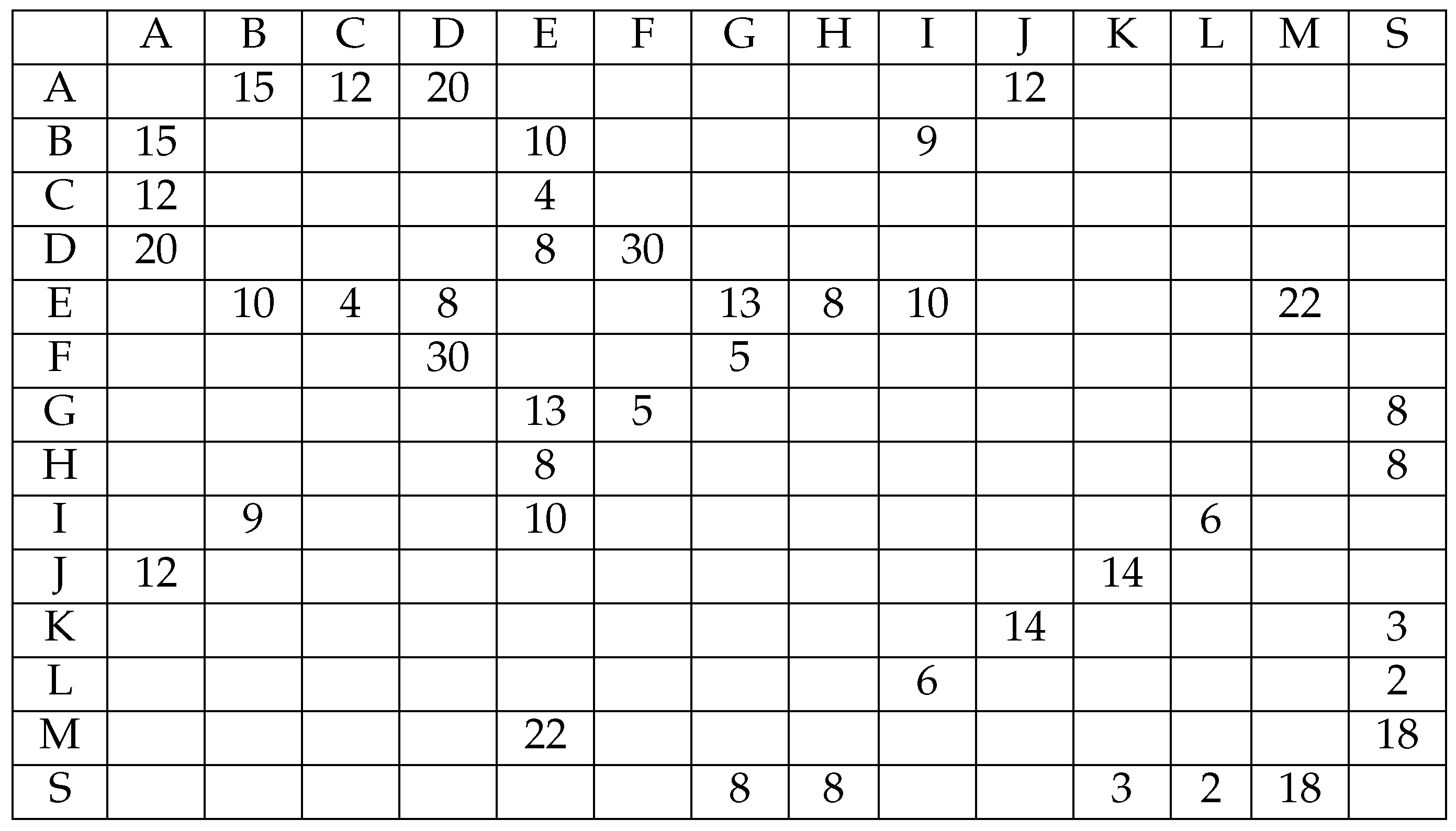
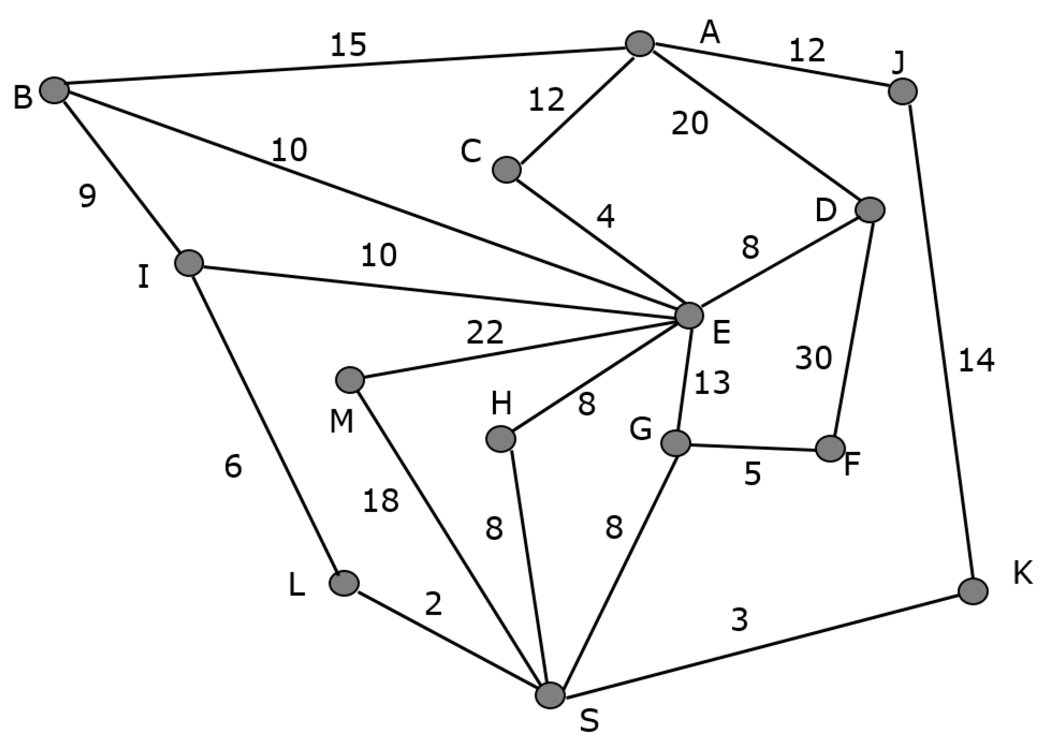
Can you find a route from A to S with the lowest gasoil consumption?
The photographer’s jeep has broken down, and he cannot fix it until one week later. He still wants to go from A to S. A friend leaves him an old car with a fuel capacity of only 20 L, although it has the same consumption per 100 km as his own. Since the capacity of the new car is lower, he wants to make sure that he will find enough gas stations along the way. Otherwise, he will have to bring a gasoil can. Since he would prefer not to carry it due to the space it occupies and how much it weighs, as well as the potential risk involved, he studies the cities of the area, the roads that connect them, and the estimated amount of fuel to cover them, as well as the locations of the gas stations. He confirms that there are open gas stations in cities A , E , F , I , K , and M. Considering the small tank of his vehicle (20 L), answer the following question:
(b)
Is there a route that allows the photographer to go from A to S without having to carry a gasoil can? If there is more than one, which route uses the least amount of fuel?
Proof. 
After the students have modeled the context of the problem as a graph G = ( V , E ) , where V = {cities} and E = { ( x , y ) with x , y V such that there is a direct road between x and y } , we ask them what will be the natural way to represent the gasoil consumption on each of the roads, which will allow us to introduce the concept of a weighted graph. Therefore, we assume that the graph is nondirected and the weight of each edge corresponds to the gasoil consumption when traveling between two cities, as can be seen in Figure 2:
(a)
The problem consists of finding the path from A to S for which we need the least gasoil consumption. Since the weights are all positive, this example serve to introduce Dijkstra’s algorithm for obtaining the path of minimum weight from A to S, which corresponds to route A J K S with a gasoil consumption of 29 L. Since the capacity of the jeep is 40 L, the photographer will arrive at city S without any problem;
(b)
In this new situation, we consider again the weighted graph from Figure 2. From the results obtained in Section (a), there is no possibility to travel from A to S directly without refueling due to the new car’s capacity since the shortest route from A to S needs 29 L of gasoil.
The problem can be analyzed as follows. We must first look for the shortest paths to all gas stations from A and analyze which of these paths are feasible. Then, in the second stage, we consider whether it is possible to reach the gas stations not reached in the previous stage by considering another path different from the shortest one. Finally, in the third stage, we look for the shortest paths from the reachable gas stations to S. Below, we explain in detail the development of these steps, pointing out the hints, clues, or observations that we use to guide the students, helping them to solve the problem.
First stage:
We first apply Dijkstra’s algorithm to graph G to determine the path with the lowest weight from A to the towns with a gas station, that is E , F , I , K , and M. The result of applying it is:
P A E = A C E with weight w ( P A E ) = 16 ;
P A F = A C E G F with weight w ( P A F ) = 34 ;
P A I = A B I with weight w ( P A I ) = 24 ;
P A K = A J K with weight w ( P A K ) = 26 ;
P A M = A C E M with weight w ( P A M ) = 38 .
Observe that the photographer can go to E without any problem since the gasoil consumption for the route A C E is 16 L. At this moment, we ask the students if it is sufficient to check if the gasoil consumption of the obtained paths is greater than 20 to discard them. We have to try to make them realize they have to analyze among all the routes those that contain an intermediate gas station.
Indeed, the routes A C E G F and A C E M contain intermediate gas stations. Therefore, we must study the two paths in which each gas station divides the route. In the case of A C E G F , the path A C E has a weight of 16 L and E G F has a weight of 18 L. Consequently, that route will be possible since the photographer can refuel in city E despite w ( P A F = 34 ) . Conversely, the route A C E M will not be possible since w ( A C E ) = 16 , but w ( E M ) = 22 > 20 .
To sum up, we can reach E and F considering the paths A C E and A C E G F with weights w ( A C E ) = 16 and w ( A C E G F ) = 34 .
Second stage:
Before further solving the problem, we point out to the students that the shortest path from A to S does not need to be the concatenation of the shortest one from A to a gas station together with the shortest path from it to S.
The shortest paths from A to I and K provided by Dijkstra’s algorithm do not contain any intermediate gas station, and they have a weight whose value is greater than 20. Consequently, I and K should be analyzed separately together with M since it could happen that by means of a longer route that included one of the gas stations E or F, it could be possible to reach them from A. We analyze them:
Gas station I: Since the graph is nondirected, we encourage the students, instead of applying Dijkstra’s algorithm to the different gas stations from which I can be reached, to apply it to I to obtain the paths:
*
P I F = I E G F with weight w ( P I F ) = 28 ;
*
P I E = I E with weight w ( P I E ) = 10 .
We note that the paths we have to analyze are E I and F G E I . In the last one, to get to I, we pass through the intermediate gas station E. Therefore, to determine whether it is valid or not, we must analyze if the corresponding subroutes have a weight smaller than 20. Indeed, since w ( F G E I ) = w ( F G E ) + w ( E I ) = 18 + 10 and both paths F G E and E I weigh less than 20, routes F G E I and E I will be possible. Since E I is shorter than F G E I , the shortest path that allows us to reach I from a gas station is P E I = E I with w ( P E I ) = 10 .
Then, the shortest route from A to I will be A C E I with a consumption of 26 L;
Gas station M: Following the same analysis as before, we look for the shortest paths from M to E and F. Applying Dijkstra’s algorithm, we obtain the following routes:
*
P M E = M E with weight w ( P M E ) = 22 ;
*
P M F = M E G F with weight w ( P M F ) = 40 .
Since the gasoil consumption along M E is greater than 20 L, this route will not be valid. On the other hand, w ( M E G F ) = w ( M E ) + w ( E G F ) = 22 + 18 , and then, M E G F cannot be considered. Consequently, the photographer will not be able to get from E or F to M;
Gas station K: We observe that all the routes from E and F to K pass through A or S, so it will not be possible to move from them to K.
At this point, following the same reasoning stated at the beginning of Stage 2, we ask the students if there are alternative routes to reach M or K from I.
The shortest route from I to M that does not pass through A or S is given by I E M with w ( I E M ) = w ( I E ) + w ( E M ) = 10 + 22 . On the other hand, all routes from I to K pass through A or S, so we discard all of them.
Combining all the previous results, the possible routes from A to a gas station are A C E , A C E I , and A C E G F with weights w ( A C E ) = 16 , w ( A C E I ) = 26 , and w ( A C E G F ) = 34 , respectively.
Third stage:
Finally, once we know the reachable gas stations, we ask the students how to obtain the solution of the problem.
We must therefore find the shortest routes from the towns E , I , and F to S. Therefore, since graph G is nondirected we can simply apply Dijkstra’s algorithm to S and obtain the shortest path to them:
P S E = S H E with weight w ( P S E ) = 16 ;
P S F = S G F with weight w ( P S F ) = 13 ;
P S I = S L I with weight w ( P S I ) = 8 .
Thus, all possible routes from A to S without the need to carry a gasoil can are A C E H S , A C E I L S , and A C E G F G S with weights w ( A C E H S ) = w ( A C E ) + w ( E H S ) = 32 , w ( A C E I L S ) = w ( A C E I ) + w ( I L S ) = 34 , and w ( A C E G F G S ) = w ( A C E G F ) + w ( F G S ) = 47 .
We will clearly recommend the photographer take route A C E H S because it is the least costly or, in other words, the one for which he will have to travel the least kilometers without having to carry the gasoil can.
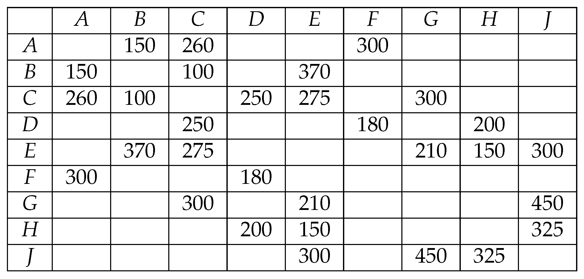
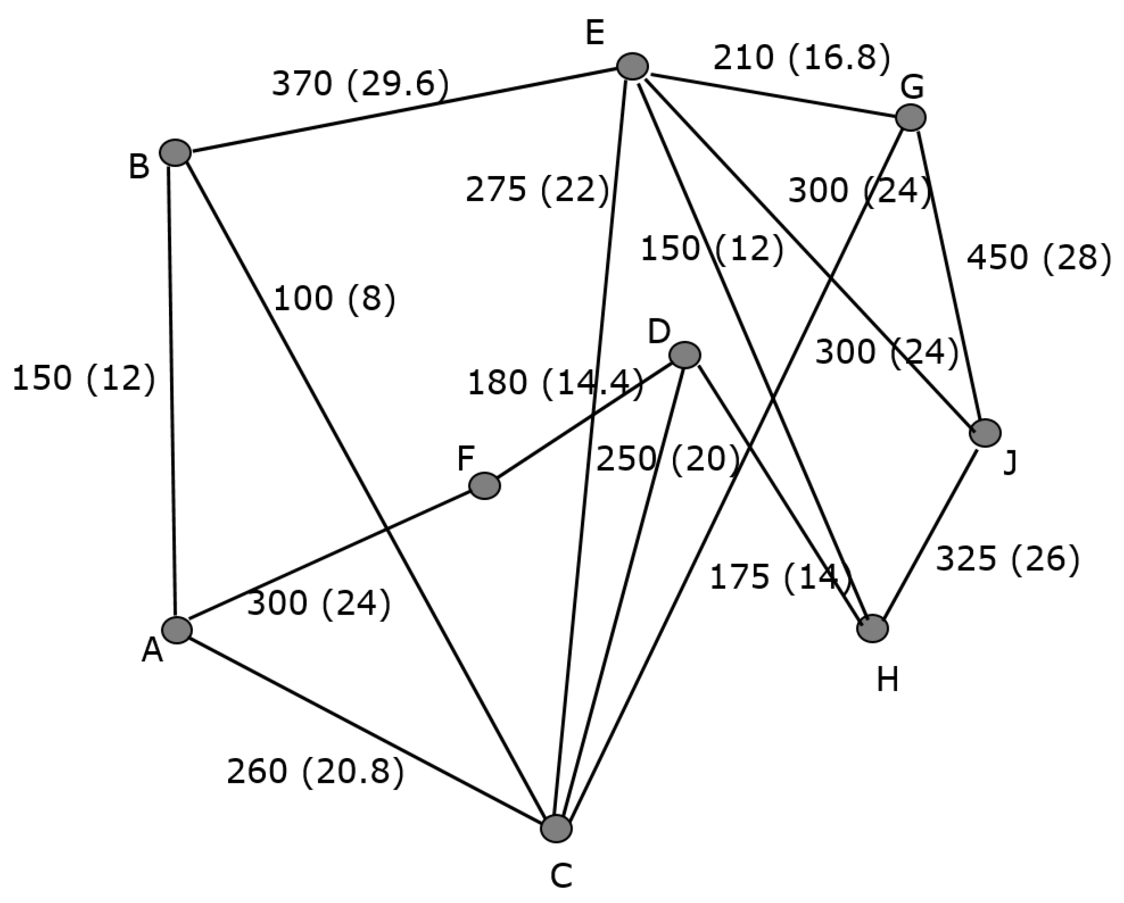
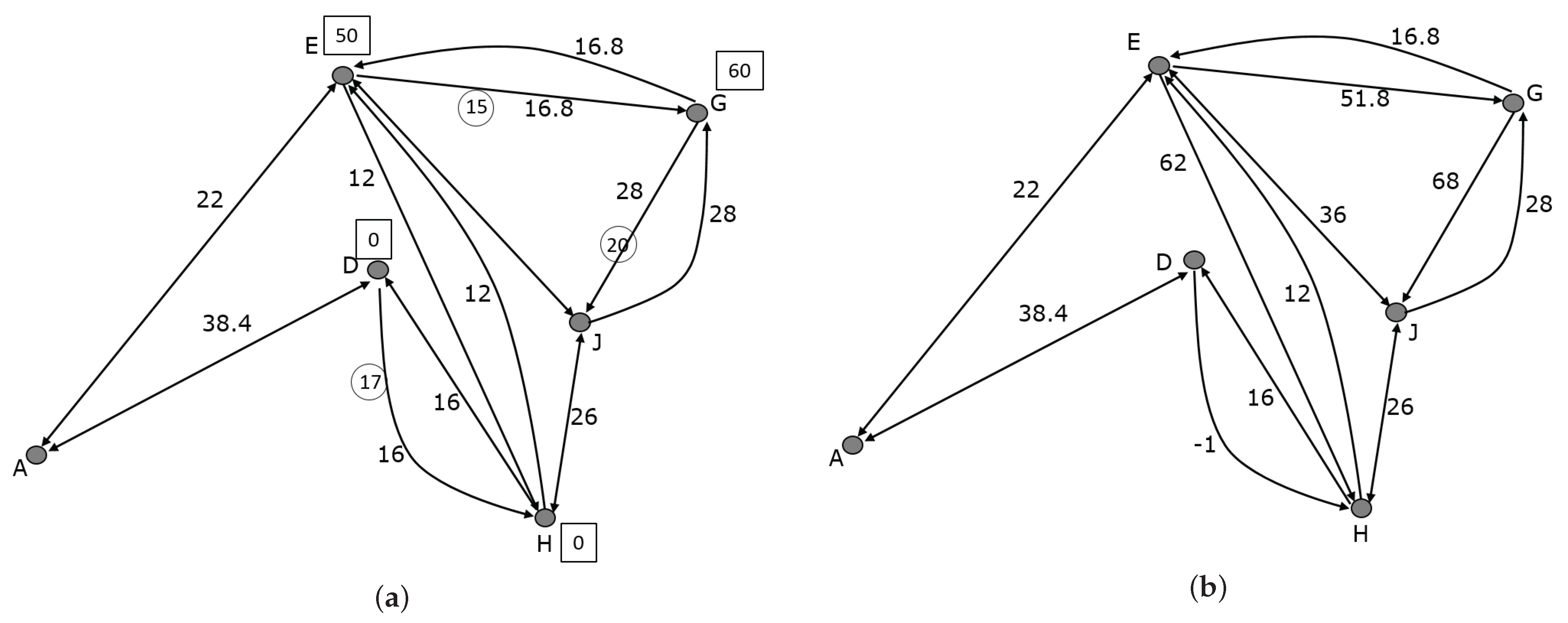
After solving the previous problem, the students are expected to be able to tackle the new problem posed below. When weighting the graph to model the situation, they should include all the restrictions about the costs/benefits that appear in the statement.
Thus, the students should realize that they should represent the costs with positive weights and, in contrast, the benefits with negative ones. As a particularity, they should note that the weight of the arc ( i , j ) does not have to coincide with that of the arc ( j , i ) , which will lead to modeling the situation using a directed graph. The graph defined will have a matrix of weights with negative values to which Dijkstra’s algorithm cannot be applied. In this way, the introduction of the Bellman–Ford algorithm is motivated.
Problem 2.
The owner of a van is going to make a trip from city A to J. Studying the map, she realizes she can make the journey by stopping to sleep in towns where she knows a friend, thereby saving the cost of accommodation. In Figure 3, the kilometers between each pair of towns are shown, and in Figure 4, the cost of accommodation in each city is collected. In addition, she has the possibility of transporting some packages of a medium and small size in the surroundings of some of the cities. The benefit that this would represent is reflected in Figure 5. She wants to travel a maximum number of kilometers on the day of departure since she wants to arrive early the next day, but due to the time at which she leaves and the obligatory rest stops, she calculates that she will be able to drive at most 525 km. On the other hand, she does not want to spend the night in B , C , or F since there are local races in these cities the next day, and they will be shut down.
If the cost of fuel is approximately EUR 8 per 100 km, determine the path she should follow and if she should accept any of the job offers to make the cost of the trip between A and J as economical as possible.
Proof. 
This problem can be analyzed in two stages. In the first one, we analyze all the possible cities she can reach the first day, given the maximum number of kilometers and the restrictions on the statement of the problem. Then, on the possible paths, we compute the minimal cost for each destination taking into account the benefits of the jobs. In the second stage, we consider a new graph for the second day, where we reflect the paths obtained in the previous step and take into consideration the accommodation cost and the job benefits without a limitation on the number of kilometers this day.
Specifically, we start the modeling of the problem by considering a graph G = ( V , E ) , where V = {cities} and E = { ( x , y ) , x , y V such that there is a direct road between x and y } . From the context of the problem, and it being most common that roads are two-way, it seems that we should assume that G is nondirected. It is necessary to make the student observe that we must reflect through the weightings the costs of accommodation and the earnings from transporting packages, so the weight assigned to the pair ( i , j ) will not always be the same as the one assigned to the pair ( j , i ) . Therefore, we must consider that G is directed. We assign G different weights as we develop the problem.
First stage:
We encourage the students to analyze the statement in order to conclude that the first thing to determine is where the owner of the van should spend the night, taking into account that she wants to travel at most 525 km before stopping to sleep.
Therefore, we assume as an initial weighting the values provided in Figure 3, relative to the kilometers between cities, where the position ( i , j ) denotes the distance in kilometers between i and j (see Figure 6). First of all, to achieve the goal of the first day in relation to the kilometers to be covered, we have to determine all routes with initial vertex A whose weight is less than 525. We discard getting from A to G , H , and J since, by Dijkstra’s algorithm, the shortest paths to these vertices have a weight greater than 525.
We ask the students if it is sufficient to calculate the shortest paths from A using Dijkstra’s algorithm, taking into account that our objective is to find the most economical route, which will be influenced by the transport benefits. As they easily see, the answer is negative, and then, the solution is obtained by comparing all possible routes departing from A and whose weight meets the desired conditions.
Thus, the owner of the van will be able to choose between the following paths: A B with 150 km, A B C with 250 km, A F with 300 km, A B E of 520 km, A B C D of 500 km, A B C E of 525 km, A C D of 510 km, and A F D of 480 km. We discard A B , A F , and A B C since she does not want to spend the night in these cities due to the local races.
In addition, in order to choose the most suitable path among the mentioned ones, we must consider whether the cost in EUR of any of the aforementioned routes can be lowered thanks to the job offers related to the transport received.
To do this, first of all, we ask the students if the previous weights reflect these benefits and costs since they should realize we have to change the costs in kilometers between two cities to costs in EUR (see Figure 6). They should transfer them into a cost matrix, which we call W e = ( w i j e ) , only taking into account the fuel price per 100 km given in the statement.
W e = [ 0 12 20.8 24 12 0 8 29.6 20.8 8 0 20 22 24 20 0 14.4 16 29.6 22 0 16.8 12 24 24 14.4 0 24 16.8 0 28 16 12 0 26 24 28 26 0 ]
In order to determine the most economical routes from A to D and from A to E among those mentioned above, we must take into account that, when accepting transport offers, going from B to E or from C to E brings her benefits. At this point, we ask the students how these benefits should be added. We show them that these benefits should be reflected as negative weights, as opposed to costs, represented by positive weights. We therefore consider a second cost matrix W D E = ( w i j D E ) whose values are equal to those of the matrix W e = ( w i j ) e except for the entries w B E D E = w B E e 15 and w C E D E = w C E e 20 . Moreover, possible accommodation expenses do not increase this cost since she will only stop to sleep in D or E.
Considering the new weighting that includes the gains, we compare the weights of the paths: A B E and A B C E , on the one hand, and A B C D , A C D and A F D , on the other. We obtain that the least costly path from A to D is A F D with weight 38.4 and from A to E is A B C E with weight 22.
We now ask the students if the most economical path from A to J can be directly obtained by considering the one with the least weight of the previous ones, that is the path A B C E , and then calculating the shortest from E up to J. We reason this conclusion is not necessarily true since we do not know the weight of the paths from D and E up to J.
Second stage:
Next, to analyze the route on the second day, we generate a new graph G , whose graphical representation can be seen in Figure 7, where the vertices B , C , F are eliminated from G and the following changes are made as follows:
  • A B C D , A C D and A F D are replaced by a unique edge A D weighted with 38.4 ;
  • A B E and A B C E are replaced by a unique edge A E weighted with 22.
The student may not consider the option of eliminating the vertices B , C , F and reconsidering this new graph G , and thus, they will need some previous help from the professor, who will emphasize the advantages of reducing the graph.
In relation to the weighting of G , we must make the students keep in mind the cost in EUR per kilometer, per accommodation, and the discount for package transport, as explained below.
To begin, we consider that each edge of this new graph is assigned the weight that we established in matrix W e except for A D and A E , whose values will be 38.4 and 22, respectively. Note that the new graph G has three fewer vertices than the original, so the matrix of weights of G will be a 6 × 6 matrix. In Figure 7, we can see the graphical representation of this new graph G with the assigned weights.
It is important that the students think about how to include the weight of the accommodation and the benefits obtained by accepting job offers in the graph. In relation to the cost of the accommodation, if it has a value of c i in the vertex i, this weight is added to that assigned to the edge with initial vertex i in the previous paragraph. This means this value will affect us if we sleep in i and then move towards j, but not if leaving j, we reach i. Consequently, we consider our graph G as a directed one.
Regarding the benefits, they should make a similar analysis of that of accommodation. The benefit is obtained if we transport the package from i to j, but not vice versa. Therefore, we have to weight the two arcs differently. Thus, if the benefit of transporting the package from i to j is b i j , we subtract it from the value assigned to the arc ( i , j ) until this moment. In case we have a double arc with the same value, it is represented by a single arc with two arrow ends.
Considering the above constraints, we weight the graph G with the matrix W given by:
W ' = [ 0 38.4 22 38.4 0 1 22 0 51.8 62 36 16.8 0 68 14 12 0 26 36 28 26 0 ]
The graphical representation of the graph G with the new weighting can be seen in Figure 7.
Now, we can compute the shortest path from A to J. As there are negative values, we emphasize that Dijkstra’s algorithm cannot be applied, and this serves to introduce the Bellman–Ford algorithm. Applying it, we obtain the shortest path as A F D H J ; the owner of the van will sleep at her friend’s house in D and will transport a package from D to H for which she will receive EUR 17, the total cost of the trip being EUR 63.4 . □
Observe that in the previous problem, we can consider new and different constraints. We could now ask the students what would happen if there were a restriction on the maximum kilometers per day assuming that there is no need to arrive at J the next day. Another option could be to ask them what would happen in case there are no local races in B , C , or F.

4. Conclusions

We consider Graph Theory to be a part of mathematics that allows the student to discover the close relationship between mathematics and many aspects of the real world, in particular our everyday environment. It is worth noting that its intuitive graphic representation allows its introduction at levels where knowledge in mathematics is limited.
However, if we want this theory to be useful, whether in STEM education or in any educational context where applicability or multidisciplinarity is sought, we must change the classical methodology. In our opinion, it is much more fruitful to start by posing problems, close to and easily understandable by the student, that allow, when trying to find their solution, introducing the different concepts of Graph Theory.
Given the multiple applications of Graph Theory in STEM disciplines, an applied approach to its teaching is necessary. In computer science, graphs are useful in network security, the optimization of database searches, the representation of communication networks, and improving the efficiency of programming, among others. In biology, they are used to study the monitoring of contagious diseases, the evolution of species, metabolic networks, etc. In physics and chemistry, their applicability stands out when describing the connections in molecular structures. In engineering, we can, for example, solve logistic and distribution problems based on Eulerian and Hamiltonian graphs and the theory of networks and flows, being also useful in the design of electrical circuits.
In the present work, we proposed two problems that may be useful for the introduction of weighted graphs and the algorithms to solve the shortest path problem, including weighted graphs with negative weights, which are very rare in the literature. Both problems incorporate trivial questions, but also others that are not, which constitutes a challenge for the student and allows us to meet the objective of developing reasoning skills.

Author Contributions

All authors declare they have equally contributed to the preparation of the paper. All authors have contributed read and agreed to the published version of the manuscript.

Funding

This research received no external funding.

Acknowledgments

The authors would like to thank the anonymous reviewers for their suggestions and comments, which have improved the quality and presentation of this manuscript.

Conflicts of Interest

The authors declare that they have no conflict of interest.

References

  1. Blinov, M.L.; Yang, J.; Faeder, J.R.; Hlavacek, W.S. Graph Theory for Rule-Based Modeling of Biochemical Networks. In Transactions on Computational Systems Biology VII; Lecture Notes in Computer Science; Springer: Berlin/Heidelberg, Germany, 2006; Volume 4230. [Google Scholar]
  2. Huber, W.; Carey, V.J.; Long, L.; Falcon, S.; Gentleman, R. Graphs in molecular biology. BMC Bioinform. 2007, 8, S8. [Google Scholar] [CrossRef] [PubMed] [Green Version]
  3. Chen, W.-K. Graph Theory and Engineering Applications; World Scientific Publishing: Singapore, 1997. [Google Scholar]
  4. Conejero, J.A.; Jordán, C.; Sanabria-Codesal, E. A tree-based model for setting optimal train fare zones. Math. Probl. Eng. 2014, 214, 384321. [Google Scholar] [CrossRef]
  5. Costa, P.C.S.; Evangelista, J.S.; Leal, I.; Miranda, P.C.M.L. Chemical Graph Theory for Property Modeling in QSAR and QSPR—Charming QSAR & QSPR. Mathematics 2021, 9, 60. [Google Scholar]
  6. Machado, J.A.T.; Mata, M.E. A fractional perspective to the bond graph modeling of world economies. Nonlinear Dyn. 2015, 80, 1839–1852. [Google Scholar] [CrossRef] [Green Version]
  7. Pedroche, F. A model to classify users of social networks based on pagerank. Int. J. Bifurc. Chaos 2012, 22, 1250162. [Google Scholar] [CrossRef]
  8. Pérez-Benito, C.; Morillas, S.; Jordán, C.; Conejero, J.A. A model based on local graphs for colour images and its application for Gaussian noise smoothing. J. Comput. Appl. Math. 2018, 330, 955–964. [Google Scholar] [CrossRef]
  9. Chai, A.; Le, J.P.; Lee, A.S.; Lo, S.M. Applying Graph Theory to Examine the Dynamics of Student Discussions in Small-Group Learning. CBE-Life Sci. Educ. 2019, 18, ar29. [Google Scholar] [CrossRef] [PubMed] [Green Version]
  10. Ramle, R.; Rosli, D.I.; Nathan, S.S.; Berahim, M. Question-led approach in designing Dijkstra algorithm game-based learning: A pilot study. Int. J. Eval. Res. Educ. 2020, 9, 926–933. [Google Scholar] [CrossRef]
  11. Sánchez-Torrubia, M.G.; Torres-Blanc, C.; Lopez-Martinez, M.A. PathFinder: A Visualization eMathTeacher for Actively Learning Dijkstra’s Algorithm. Electron. Notes Theor. Comput. Sci. 2009, 224, 151–158. [Google Scholar] [CrossRef] [Green Version]
  12. Chen, P.; Chiou, P.; Young, G. A Study of Learning Effectiveness on the Dijkstra’s Algorithm Modeled in an Interactive KLA Approach. In Proceedings of the 13th International Conference on Frontiers in Education: Computer Science and Computer Engineering (FECS’17), Las Vegas, NV, USA, 17–20 July 2017; pp. 234–238. [Google Scholar]
  13. Bang-Jensen, J.; Gutin, G. Digraphs-Theory, Algorithms and Applications; Springer: Berlin/Heidelberg, Germany, 2002. [Google Scholar]
  14. Chartrand, G.; Oellerman, O.R. Applied and Algorithmic Graph Theory; McGraw Hill: New York, NY, USA, 1993. [Google Scholar]
  15. Gross, J.L.; Yellen, J. Graph Theory and Its Applications; CRC Press: Boca Raton, FL, USA, 2006. [Google Scholar]
Figure 1. Gasoil consumption in liters when traveling between cities.
Mathematics 09 03110 g001
Figure 2. Graphical representation of the nondirected weighted graph G whose weights denote the gasoil consumption between cities.
Mathematics 09 03110 g002
Figure 3. Distances in kilometers between cities.
Mathematics 09 03110 g003
Figure 4. Cost of accommodation in cities.
Mathematics 09 03110 g004
Figure 5. Benefit of transporting a package between two points of the road that directly connect cities i and j, which is represented as i j .
Mathematics 09 03110 g005
Figure 6. Graphical representation of the nondirected weighted graph G whose weights denote the kilometers between cities (and the corresponding fuel cost in EUR between parentheses).
Mathematics 09 03110 g006
Figure 7. Graphical representation of the graph G reflecting: (a) the costs provided in the statement of the problem and (b) the cost of each arc already calculated.
Mathematics 09 03110 g007
Publisher’s Note: MDPI stays neutral with regard to jurisdictional claims in published maps and institutional affiliations.

