A Novel Trading Strategy Framework Based on Reinforcement Deep Learning for Financial Market Predictions

Abstract

The prediction of stocks is complicated by the dynamic, complex, and chaotic environment of the stock market. Investors put their money into the financial market, hoping to maximize profits by understanding market trends and designing trading strategies at the entry and exit points. Most studies propose machine learning models to predict stock prices. However, constructing trading strategies is helpful for traders to avoid making mistakes and losing money. We propose an automatic trading framework using LSTM combined with deep Q-learning to determine the trading signal and the size of the trading position. This is more sophisticated than traditional price prediction models. This study used price data from the Taiwan stock market, including daily opening price, closing price, highest price, lowest price, and trading volume. The profitability of the system was evaluated using a combination of different states of different stocks. The profitability of the proposed system was positive after a long period of testing, which means that the system performed well in predicting the rise and fall of stocks.

1. Introduction

Market forces cause stock prices to change every day. Influencing the stock market are uncertain factors caused most notably by political issues and the government. Such uncertainty complicates the determination of appropriate trading strategies for selling or buying stock. Stock market analysis includes portfolio optimization [1], investment strategy determination [2], and market risk analysis [3]. Stock price trend prediction has attracted researchers and participants from various disciplines, such as economics, financial engineering, statistics, operations research, and machine learning [4,5,6].

Traditional studies have proposed algorithms to predict stock trends based on machine learning techniques, such as artificial neural networks (ANNs) and support vector machines (SVMs) [5,6,7,8]. Recently, scholars have begun to adopt well-known deep learning techniques, such as recurrent neural networks (RNNs) and long short-term memory (LSTM) networks [9,10], for stock price prediction. Designing a profitable stock trading strategy is a challenging issue in financial market research, as financial time series data is highly volatile and noisy. Traditional traders must analyze large amounts of data to decide whether to place empty orders, multiple orders, or no transactions. In addition, after deciding to make a single order, to maximize profits, they must decide the size of the transaction. Recently, some researchers have proposed trading algorithms to maximize profits [3].

Reinforcement learning and Q-learning are machine learning algorithms for automating goal-directed learning and decision making [11]. Moody and Saffell [12] optimized portfolios and trading stocks using direct reinforcement learning. Using reinforcement learning, Deepmind learned to play seven Atari video games, even achieving human-expert level on three of them. The system later achieved a human-expert level in over 20 different Atari games [13]. AlphaGo, that combines neural networks and reinforcement learning, beat the best Go player in the world, boosting the popularity of reinforcement learning applied in deep learning as a topic of research.

In this study, we propose a novel automatic trading system which combines deep learning and reinforcement learning to determine the trading signal and the size of the trading position. The system is constructed from an LSTM network combined with deep Q-learning, which is an off-policy reinforcement learning algorithm that seeks to find the best action to take given the current state. It is considered off-policy because the Q-learning function learns from actions that are outside the current policy, such as random actions, and therefore no policy is needed. More specifically, Q-learning seeks to learn a policy that maximizes the total reward. Our system is based on the deep Q-network [14]. We verify this system with five different financial products and three different states. The paper is organized as follows. In Section 2, we review related work, and in Section 3 we introduce our methodology. Our experimental data and results are presented in Section 4. We conclude in Section 5.

2. Literature Review

Stock market prediction had been proposed by many researchers using several machine learning techniques [15,16,17,18,19]. Recently, deep learning models have been a popular research issue [20,21,22] and we briefly discuss previous applications of deep learning to financial trading. Ding et al. [23] proposed a deep convolutional neural network using event embedding which combined the influence of long-term events and short-term events to predict stock prices. Their events included stock price changes over months, weeks, and days. They demonstrated that combining event embedding with deep convolutional networks is useful for stock price prediction.

Akita et al. [24] built an LSTM model using textual and numerical information to predict ten company’s closing stock prices. The experimental results showed that combining textual and numerical information was better than methods that use only textual data or only numerical data. Nelson, Pereira, and de Oliveira [25] proposed a model based on LSTM using five historic price measures (open, close, low, high, and volume) and 175 technical indicators to predict stock price movement.

Liu et al. [26] predicted stock price movements using a novel end-to-end attention-based event model. They proposed the ATT-ERNN model to exploit implicit correlations between world events, including the effect of event counts and short-term, medium-term, and long-term influence, as well as the movement of stock prices. Qin [27] forecasted time series using a novel dual-stage attention-based recurrent neural network (DA-RNN) which consisted of an encoder with an input attention mechanism and a decoder with a temporal attention mechanism.

Fischer and Krauss [9] applied an LSTM model to a large-scale financial market prediction task on S&P 500 data from December 1992 to October 2015. They showed that the LSTM model outperformed standard deep net and traditional machine learning methods. Zhao et al. [28] captured market dynamics from multimodal information (fundamental indicators, technical indicators, and market structure) for stock return prediction by using an end-to-end market-aware system. Their market awareness system led to reduced error, and temporal awareness across stacks of market images led to further error reductions.

In reinforcement learning (RL), the model learns to map situations to actions to maximize the reward [29]. The RL agent is not instructed explicitly about how to improve its learning [14]; instead, the agent only observes state information from its environment. The agent then learns by itself to select actions given this state and the reward obtained.

A reinforcement learning system includes a policy, a reward, a value function, and an environment. At each time step t = 0, 1, 2, 3, …, the agent and environment interact with each other; the agent observes st ∈ S, where S is the set of possible states from the environment, and then selects an action, at ∈ A(st), where A(st) is the set of actions that may be executed in state st. In the next time step, the agent receives a reward, rt + 1 ∈ ℜ, and observes a new state, st + 1. The agent’s policy is its mapping from states to actions at each time step. A policy is denoted πt, where πt (s, a) is the probability that at = a if st = s. Reinforcement learning is how the agent improves its policy given its experience. The agent’s goal is the maximum reward over the long term.

Moody and Saffell [12] introduced recurrent reinforcement learning (RRL), a direct reinforcement approach that outperformed a Q-learning implementation. Their RRL trader uses a one-layer NN to maximize a function of risk-adjusted profit, which takes as input the past eight returns and its previous output. The trader was tested on USD/GBP currency pair data, half-hourly from January 1996 to August 1996, achieving an annualized profit of 15%. Gold [30] further tested RRL on other currency markets with half-hourly data for the entire year of 1996, achieving a varied profit from −82.1% to 49.3%, with an average of 4.2% over ten different currency pairs. Duerson et al. [31] used two techniques based on recurrent reinforcement learning (RLL) and two based on Q-learning for the problem of investment strategy determination. They combined reinforcement learning and a trading system. Traditionally, stock prediction and transactions are separated into independent systems as forecaster and trader systems. They demonstrated strong performance for the Q-learning approach: on some data series, the results were twice as good as the buy-and-hold strategy. Nevmyvaka et al. [32] reported on the first extensive empirical application of reinforcement learning (RL) to the problem of optimized execution using large-scale NASDAQ market microstructure datasets. They used historical INET records and conducted experiments on three stocks—Amazon (AMZN), Qualcomm (QCOM), and NVIDIA (NVDA)—showing that RL beat the submit and leave (S&L) policy, which was already an improvement over a simple market order.

Dempster and Leemans [33] used adaptive reinforcement learning (ARL) on the currency market. In their system, they added a risk management layer and a dynamic hyper-parameter optimization layer. They tested the system on two years of EUR/USD historical data, from January 2000 to January 2002, with 1-min granularity, achieving an average 26% annual return. Lee et al. [34] proposed a new stock trading system based on reinforcement learning. MQ-trader, the proposed framework, consists of four cooperative Q-learning agents: buy and sell signal agents, which use global trend prediction to determine when to buy or sell stock shares, and buy and sell order agents, which decide the best buy price (BP) and sell price (SP) to execute intraday orders. Lee applied the four-agent approach to KOSPI 200, which includes 200 major Korean stocks. When using stock data from the Korean stock market, they found that their systems yielded better performance than other baseline systems.

Cumming et al. [35] introduced an RL trading algorithm based on least-squares temporal difference (LSTD). Their state signal consisted of the open, highest, lowest, and close prices (bid only) from the last 8 periods, where each period covers a minute. The reward was defined as the profit from each transaction. In experiments, their method achieved a 1.64% annualized profit on the EUR/USD pair market. Deep reinforcement learning methods combined with different trading strategies have become popular [36,37] and been evaluated for their robustness and effectiveness on different countries’ stock markets. The proposed three-layered multi-ensemble approach performed better than a conventional buy-and-hold strategy [38]. The three layer-stock framework, including a stacking layer, reinforcement meta learner, and ensembling layer, was evaluated with the experimental dataset containing S&P500, J.P. Morgan and Microsoft stocks between 1 January 2012 and 31 December 2019. The proposed ensemble method led to better trading results and less overfitting. The final return was better than the benchmark. Recently, a novel multi-agent deep reinforcement learning approach for stock trading was proposed and evaluated with an S&P500 dataset using walk-forward methodology. The experiment results showed that the multi-agent deep reinforcement learning approach performed better than a conventional buy-and-hold strategy [39]. This study will use this method as the base line.

3. Methodology

Reinforcement learning (RL) is learning what to do, i.e., how to map situations to actions, to maximize a numerical reward signal. Unlike supervised learning, the RL agent never receives examples of correct or incorrect performance to boost learning [24]. Instead, the agent is only provided with state information from its environment. The agent then learns to act through state. It learns what action is the best from rewards obtained for trying different actions by itself. The agent’s only goal is to maximize the rewards it gets.

We propose a framework to determine trading signals to maximize the total profit depending on the Q-value at each moment. In our framework, we modify the deep Q-learning algorithm on the stock market proposed by Mnih [24]. They combined deep neural networks and Q-learning to master difficult control policies for Atari 2600 computer games.

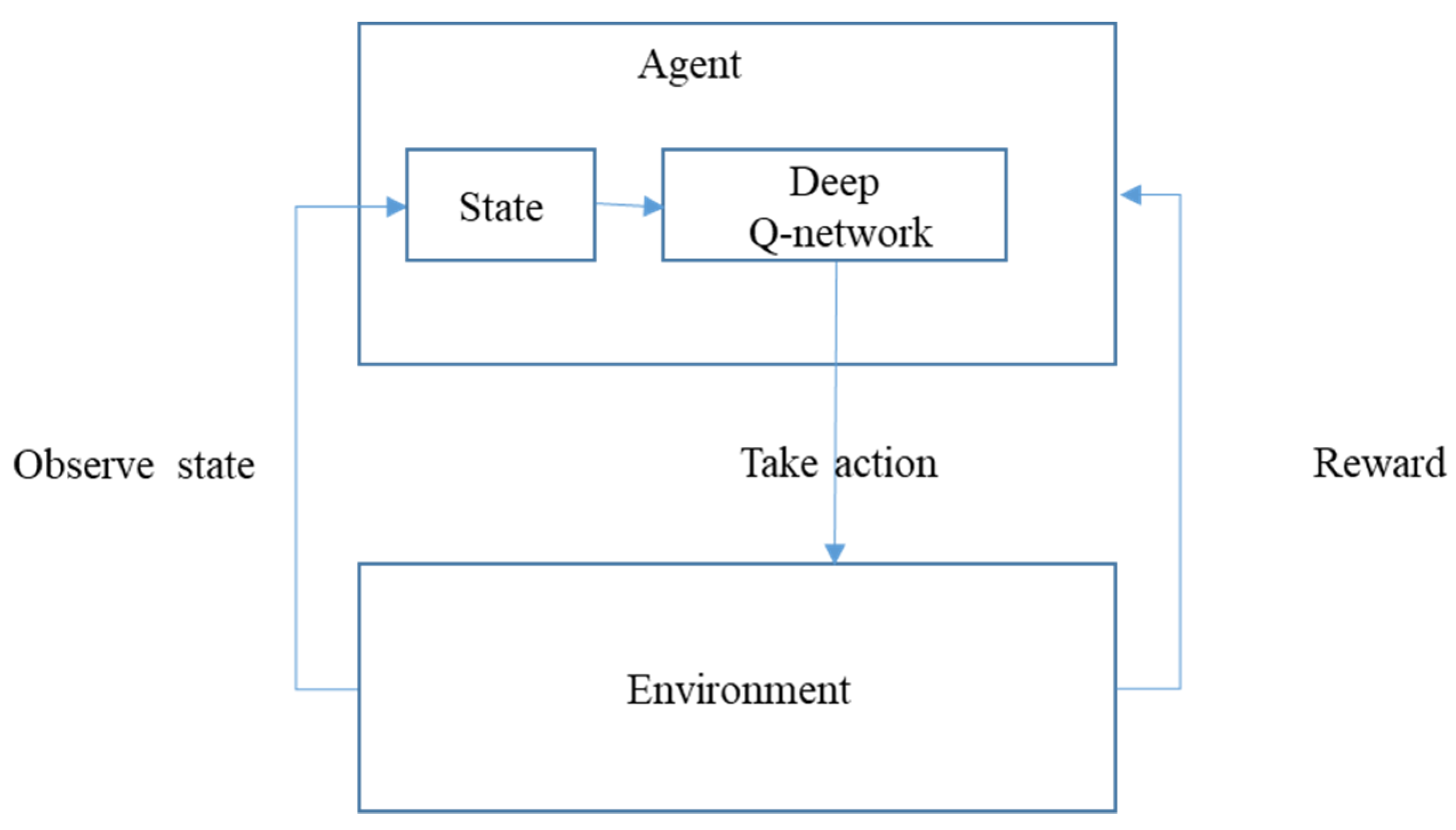
Figure 1 shows our proposed framework. A reinforcement learning system includes four main elements: a policy, a reward signal, a value function, and, optionally, a model of the environment. More specifically, the agent and environment interact at each of a sequence of discrete time steps, t = 0, 1, 2, 3, … At each time step t, the agent receives some representation of the environment’s state, s_t ∈ S where S is the set of possible states, and on that basis selects an action, a_t ∈ A(s_t), where A(s_t) is the set of actions available in state s_t. One time step later, in part as a result of its action, the agent receives a numerical reward, r_t+1 ∈ ℜ, and finds itself in a new state, s_t+1. At each time step, the agent implements a mapping from states to probabilities of selecting each possible action. This mapping is called the agent’s policy and is denoted π_t where π_t (s, a) is the probability that a_t = a if s_t = s. Reinforcement learning methods specify how the agent changes its policy as a result of its experience. The agent’s goal, broadly speaking, is to maximize the total amount of reward it receives over the long run.

At each moment, the agent observes the state from the environment and then decides what action to take using the deep Q-network. After taking an action, the agent receives a reward. Detailed definitions of the states, actions, and reward of each agent and the deep Q-network are provided in the following sections.

3.1. State Signal

Consider the stocks in time interval $\left[1,\dots ,T\right]$. Denote $O{P}_t$,$H{P}_t$,$L{P}_t$,$C{P}_t, V{O}_t$ as the open price, highest price, lowest price, close price, and volume of stock at time $t$, respectively. Note that the time interval between $t-1$ and $t$ represents one day, one week, or one month. In this paper, we consider the gross returns of these five features as the input of Q-learning. The symbols of gross returns are defined as $O_t=\frac{O{P}_t-O{P}_{t-1}}{O{P}_{t-1}}$, $H_t=\frac{H{P}_t-H{P}_{t-1}}{H{P}_{t-1}}$, $C_t=\frac{C{P}_t-C{P}_{t-1}}{C{P}_{t-1}}$, $L_t=\frac{L{P}_t-L{P}_{t-1}}{L{P}_{t-1}}$, $V_t=\frac{V{O}_t-V{O}_{t-1}}{V{O}_{t-1}}$, respectively.

Let

$$S=\left\{S_{1,5},S_{1,10},S_{1,20},S_{2,5},S_{2,10},S_{2,20},\dots ,S_{t,5},S_{t,10},S_{t,20},\dots ,S_{T,5},S_{T,10},S_{T,20}\right\}$$

be the collection of state signals, where $S_{t,5}$,$S_{t,10}$, and $S_{t,20}$ represent.

$S_{t,5}=\left[\begin{array}{c}\begin{array}{c}{O}_{t-4}, H_{t-4},L_{t-4},C_{t-4},V_{t-4}\\ O_{t-3}, H_{t-3},L_{t-3},C_{t-3},V_{t-3}\end{array}\\ O_{t-2}, H_{t-2},L_{t-2},C_{t-2},V_{t-2}\\ O_{t-1}, H_{t-1},L_{t-1},C_{t-1},V_{t-1}\\ O_t, H_t, L_t, C_t, V_t\end{array}\right]$, $S_{t,10}=\left[\begin{array}{c}\begin{array}{c}{O}_{t-9}, H_{t-9},L_{t-9},C_{t-9},V_{t-9}\\ O_{t-8}, H_{t-8},L_{t-8},C_{t-8},V_{t-8}\end{array}\\ \dots \\ \dots \\ O_{t-1}, H_{t-1},L_{t-1},C_{t-1},V_{t-1}\\ O_t, H_t, L_t, C_t, V_t\end{array}\right]$, and $S_{t,20}=\left[\begin{array}{c}\begin{array}{c}{O}_{t-19}, H_{t-19},L_{t-19},C_{t-19},V_{t-19}\\ O_{t-18}, H_{t-18},L_{t-18},C_{t-18},V_{t-18}\end{array}\\ \dots \\ O_{t-1}, H_{t-1}, L_{t-1}, C_{t-1}, V_{t-1}\\ O_t, H_t, L_t, C_t, V_t\end{array}\right]$, respectively.

The main components of the state signal S_t ∈ S, where S is a set of states {s₁, s₂, s₃, …}, are features extracted from market data, including open price, highest price, close price, lowest price, and volume. Each state S_t includes k ∈ {5, 10, 20} days of stock data. Each feature is normalized to the range [−1, 1]:

$$\begin{gathered} S_t=[\left[O_{t-k+1}, H_{t-k+1},C_{t-k+1},L_{t-k+1},V_{t-k+1}\right], \\ .... \end{gathered}$$

(1)

$$\left[O_{t-2}, H_{t-2},C_{t-2},L_{t-2},V_{t-2}\right], \left[O_{t-1}, H_{t-1},C_{t-1},L_{t-1},V_{t-1}\right], \left[O_t, H_t,C_t,L_t,V_t\right]]$$

(2)

where

$$O_t=\frac{O{P}_t-O{P}_{t-1}}{O{P}_{t-1}}, H_t=\frac{H{P}_t-H{P}_{t-1}}{H{P}_{t-1}}, C_t=\frac{C{P}_t-C{P}_{t-1}}{C{P}_{t-1}},$$

(3)

$$L_t=\frac{L{P}_t-L{P}_{t-1}}{L{P}_{t-1}}, V_t=\frac{V{O}_t-V{O}_{t-1}}{V{O}_{t-1}},$$

(4)

where OP_t is the open price at time t, HP_t is the highest price at time t, CP_t is the close price at time t, L_t is the lowest price at time t, and V_t is the volume at time t.

3.2. Trading Strategy

There are five actions, denoted as $\mathrm{Act}=\left\{{\mathrm{a}}_{\mathrm{LL}},{\mathrm{a}}_{\mathrm{LS}},{\mathrm{a}}_{\mathrm{Sit}},{\mathrm{a}}_{\mathrm{SS}},{\mathrm{a}}_{\mathrm{SL}}\right\}$ for agents in the proposed model. These actions represent long large size (${\mathrm{a}}_{\mathrm{LL}}$), long small size (${\mathrm{a}}_{\mathrm{LS}}$), sit (${\mathrm{a}}_{\mathrm{Sit}}$), short small size (${\mathrm{a}}_{\mathrm{SS}}$), and short large size (${\mathrm{a}}_{\mathrm{SL}}$), respectively. The input of our training model at time $\mathrm{t}$ is the state ${\mathrm{S}}_{\mathrm{t},\mathrm{k}}\in \mathrm{S}$. According to the state ${\mathrm{S}}_{\mathrm{t},\mathrm{k}}$ the model determines the one action in $\mathrm{Act}$ at time $\mathrm{t}$.

The proposed agent can take only five different actions: long large size, long small size, sit, short small size, and short large size. The action signal can be simplified to A(s) = $[{\mathrm{a}}_{\mathrm{LL}},{\mathrm{a}}_{\mathrm{LS}},{\mathrm{a}}_{\mathrm{Sit}},{\mathrm{a}}_{\mathrm{SS}},{\mathrm{a}}_{\mathrm{SL}}$] ∀s ∈ S, where $[{\mathrm{a}}_{\mathrm{LL}},{\mathrm{a}}_{\mathrm{LS}},{\mathrm{a}}_{\mathrm{Sit}},{\mathrm{a}}_{\mathrm{SS}},{\mathrm{a}}_{\mathrm{SL}}$] are interpreted by the environment as desired in

Table 1. Interpretation of each action.

Signal	Action	Size	Reward
$a_{LL}$	Long	Large (2 units)	$2\ast (O{P}_{t+1}-C{P}_t$)
$a_{LS}$	Long	Small (1 unit)	$1\ast (O{P}_{t+1}-C{P}_t$)
$a_{Sit}$	Sit	0	0
$a_{SS}$	Short	Small (1 units)	$1\ast (C{P}_t-O{P}_{t+1}$)
$a_{SS}$	Short	Large (2 units)	$2\ast (C{P}_t-O{P}_{t+1}$)

. If the action signal is a0 or a1, we open a long position. If the action signal is a2, we do nothing (sit). If the action signal is a3 or a4, we open a short position.

Our trading strategy is long (short) stock at the moment before the market closes and clean the position at the moment the market opens on the next day. For example, if we long the stock with closed price $C{P}_t$ on day $t$, we clean (short) the stock the next day at the price $O{P}_t$. The profit and loss on day $t$ is calculated as $C{P}_{t+1}-O{P}_t$. In this study, we represent the five actions about the positions with different sizes, where $a_{LL}$ represents two long units of stock, $a_{LS}$ represents one long unit of stock, $a_{Sit}$ represents do nothing, $a_{SS}$ represents one short unit of stock, and $a_{SL}$ represents two short units of stock.

Our trading strategy is day trading within two days. We open the position with trading price $C_t$, closed price at time t, and then close the position at time t + 1 with trading price $O_{t+1}$, open price at time t + 1. We observe k ∈ {5, 10_, 20} days of open price, highest price, close price, lowest price, and volume and then decide to open a long position or open a short position at time t. Further, we close the position at time t + 1. In addition to the trading signal, our deep Q-network also determines the position size, that is, either small or large. In other words, the agent decides what action to take using the deep Q-network after knowing the state and then executes the transaction at time t. The environment returns a reward at time t + 1.

In the classical Q learning approach, we must give the state and action as an input resulting in a Q value for that state and action. Replicating this approach in neural networks is problematic as one must give the model the state and action for each possible action of the agent, leading to many forward passes in the same model. Instead, the model is designed in such a way that it predicts Q values for each action for a given state. As a result, only one forward pass is required. The implementation of DQN for our model is similar to the Q learning method. To start, instead of initializing the Q matrix, the model is initialized. In the ϵ greedy policy, instead of choosing the action based on policy π, Q values are calculated according to the model. At the end of every episode, the model is trained using random mini batches of experience.

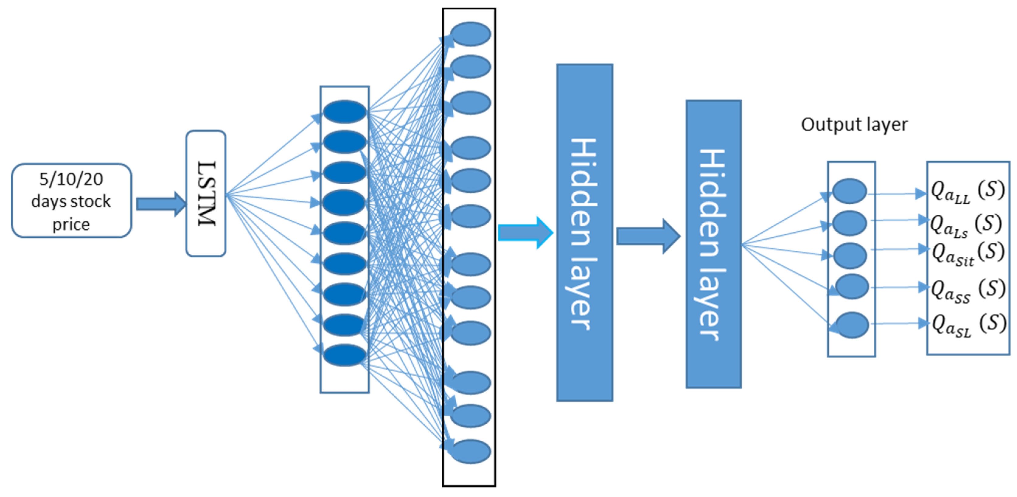
The core of the framework is a deep neural network, schematically depicted in Figure 2. This network is tasked with computing the action value for the market environment. The input layer has a number of neurons defined by the elements in our state signal, which includes k ∈ {5,10,20} [6] days of normalized open price, highest price, close price, lowest price, and volume. This input layer is followed by five hidden layers.

The first hidden layer is a long short-term memory (LSTM) layer. LSTM is chosen because it is one of the most advanced deep learning architectures for financial tasks (Fischer & C. Krauss, 2018). The remaining hidden layers are fully connected deep neural network (DNN) layers.

The output layer has five neurons to represent action values ($Q_{a_{LL}}\left(S\right),Q_{a_{Ls}}\left(S\right),Q_{a_{Sit}}\left(S\right),Q_{a_{SS}}\left(S\right),Q_{a_{SL}}\left(S\right)$), where $Q_{a_{LL}}\left(S\right)$ represents the prediction Q-value based on state and action $a_{LL}$, $Q_{a_{Ls}}\left(S\right)$ that for state and action $a_{Ls}$, $Q_{a_{Sit}}\left(S\right)$ that for state and action $a_{Sit}$, $Q_{a_{SS}}\left(S\right)$ that for state and action $a_{SS}$, and $Q_{a_{SL}}\left(S\right)$ that for state and action $a_{SL}$.

We choose the maximize action value as our action. The deep Q-network is initialized with a random set. As the network interacts with the market environment in a training process, it collects and stores state, action, and reward in memory. After a fixed period, we update the deep Q-network using the mean squared error (MSE) between the reward and action value received from the neural network.

4. Experiment

We collected two different types of financial data to verify the proposed system. Data descriptions are shown in

Table 2. Data descriptions.

Code	Name	Type	Highest Price	Lowest Price	Period
0050	Yuanta/P-shares Taiwan Top 50 ETF	ETF	90	50	January 2016–December 2018
1101	Taiwan Cement Corp	Stock	47	25	January 2016–December 2018
2330	TSMC	Stock	265	130	January 2016–December 2018
2881	Fubon Financial Holding Co, Ltd.	Stock	43	18	January 2016–December 2018
00655L	Cathay FTSE China A50 Daily Leveraged 2× ETF	ETF	48	20	March 2016–December 2018
00672L	Yuanta S&P GSCI Crude Oil 2× Leveraged ER Futures ETF	ETF	35	21	October 2016–December 2018

. These six financial products can have different patterns during the same period. The accumulated profit of these products are shown in Figure 3, Figure 4, Figure 5, Figure 6, Figure 7 and Figure 8. Code 0050 and TSMC have the same pattern because 0050 holds 18.78% of TSMC stock. Although 1101 does not show an increasing or decreasing trend, it is more volatile than 0050 and TSMC.

Codes 00655L and 00672L are leveraged ETFs, which is a security that seeks to multiply or invert the daily return of financial derivatives or debts. Code 00655L tracks the twice-daily performance of the FTSE China A50 index, and 00672L tracks the performance of the S&P GSCI Crude Oil 2× Leveraged Index ER.

We chose 0050 because the fund’s constituents are selected from the top 50 listed stocks on the Taiwan Stock Exchange by market weight, including 1101, 2330 and 2881. We also chose 00655L and 00672L because leveraged ETFs have high volatility.

4.1. Results and Discussion

Our results are presented in two stages. First, we compared the performance of the LSTM network with the deep neural network and the RNN network, and then we chose the best-performing network to construct the proposed framework. Second, we conducted various experiments to verify the proposed framework. In this experiment, we used a rolling window to evaluate the proposed approach. Each window included a three-month training period and a one-month testing period (3 months/1 month).

The key task of the proposed framework is to accurately predict stock and to determine the action to take. In this section, we used different neural networks to predict stock price movement. The input layer of the neural networks matches our state, such that the input data includes the open price, highest price, close price, lowest price, and volume. The output layer is a classification layer. As shown in

Table 3. Performance of stock price movement.

	Accuracy	Precision	Recall	F1-Measure
0050
LSTM	0.8594	0.8696	0.8333	0.9091
RNN	0.8750	0.8824	0.8333	0.9375
DNN	0.8643	0.8708	0.835	0.91
2330
LSTM	0.8630	0.8728	0.8595	0.8564
RNN	0.7697	0.7843	0.7763	0.7694
DNN	0.8519	0.8547	0.8658	0.8538
1101
LSTM	0.8772	0.9090	0.8173	0.8567
RNN	0.8438	0.8718	0.8947	0.8500
DNN	0.8112	0.8014	0.8001	0.7964
0065L
LSTM	0.9318	0.9174	0.8889	0.9143
RNN	0.9218	0.9174	0.9214	0.9179
DNN	0.8125	0.8750	0.7778	0.8235
00672L
LSTM	0.9390	0.9260	0.9572	0.938
RNN	0.9062	0.9200	0.9583	0.9388
DNN	0.9022	0.8835	0.9292	0.9020

, we achieved at least 77% accuracy in all models. LSTM outperformed other models in four of five different stocks. Hence, we used LSTM to construct the deep Q-network.

4.2. Analysis of Deep Q-Learning Performance

We conducted various experiments to verify the proposed systems using five different stocks and three different states (5, 10, and 20 days of OHCLV). We assumed initial investment funds of 100,000. We used our framework to trade 0050, 2330, and 1101 from April 2016 to December 2018, 00655L from July 2016 to December 2018, and 00672L from January 2017 to December 2018.

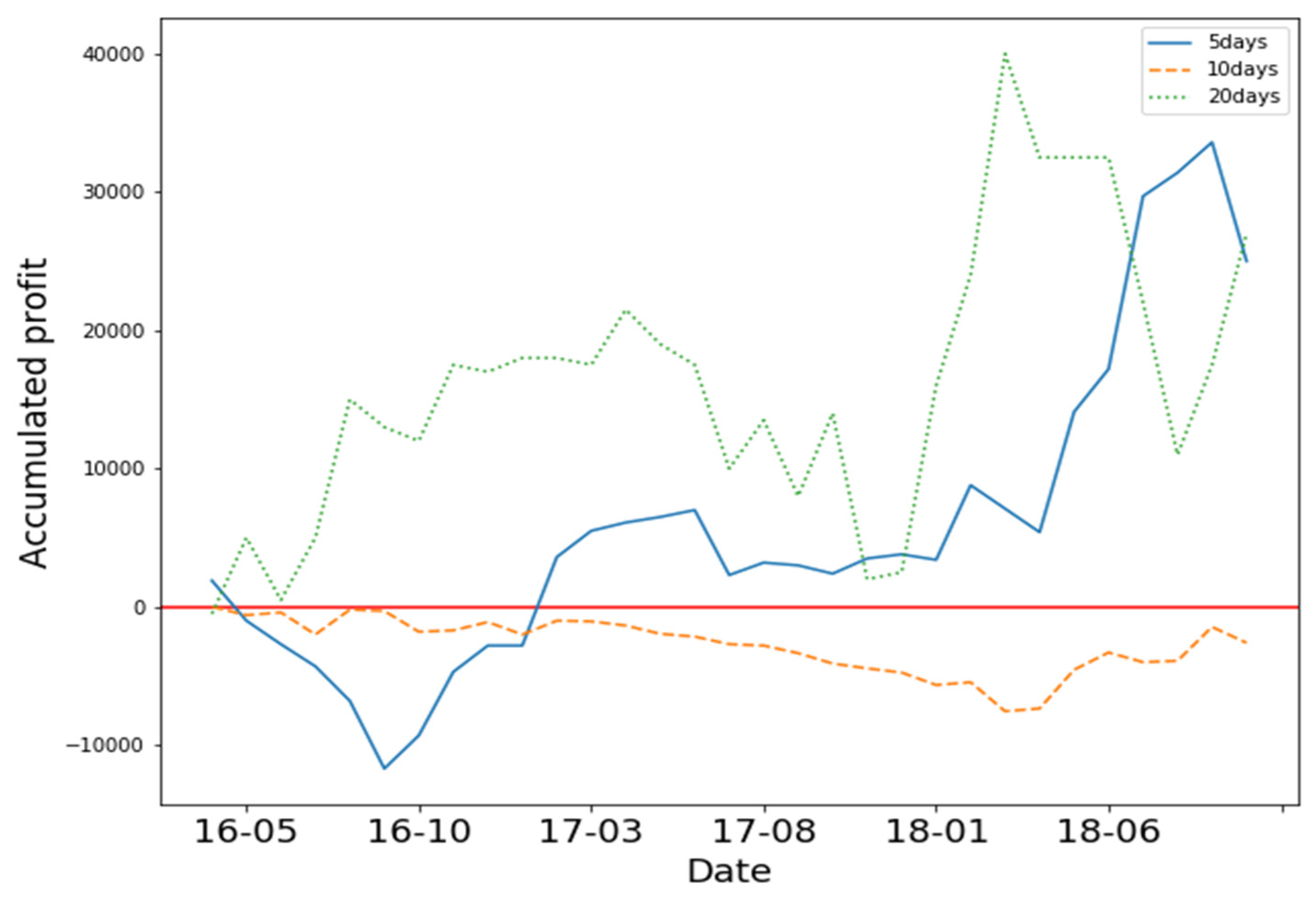
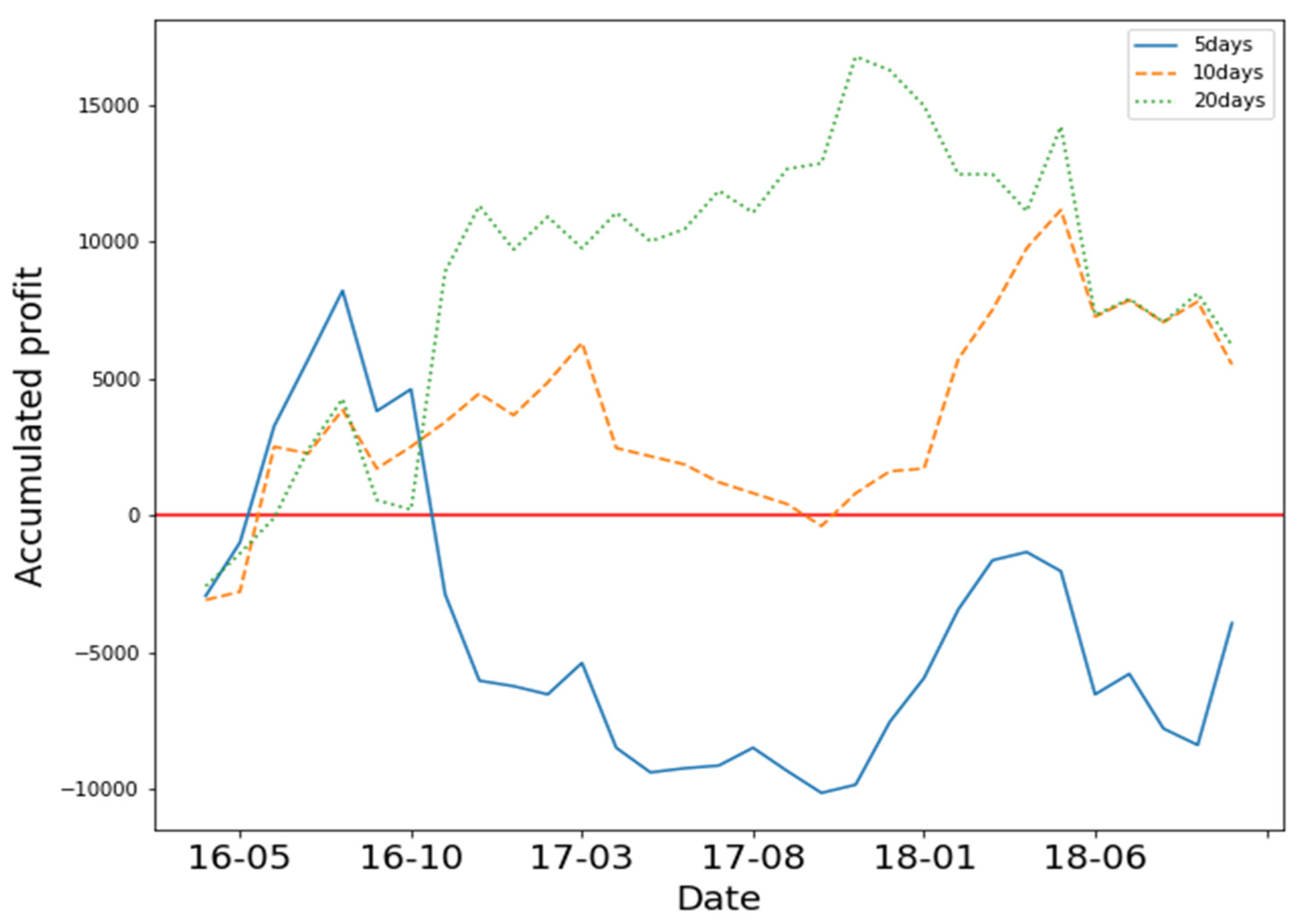
In Figure 3, the Y axis represents accumulated profit, and the X axis represents time. The three different lines represent the accumulated profit of the three different states. The results show that 5-day and 20-day states yielded positive profit. The 10-day states yielded negative profit. We found that training the model with 5 days of OHCLV on 0050 yielded the best performance.

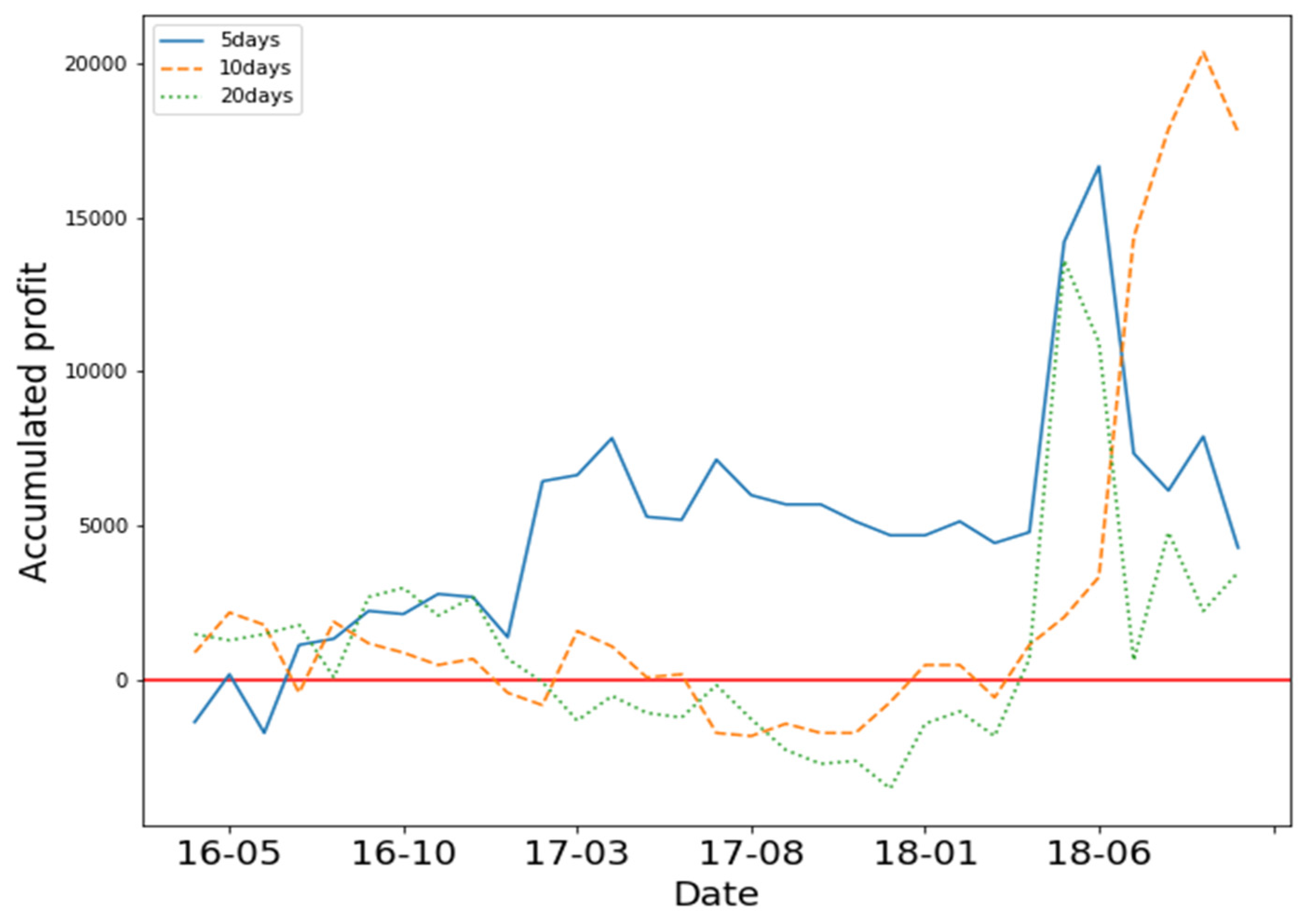
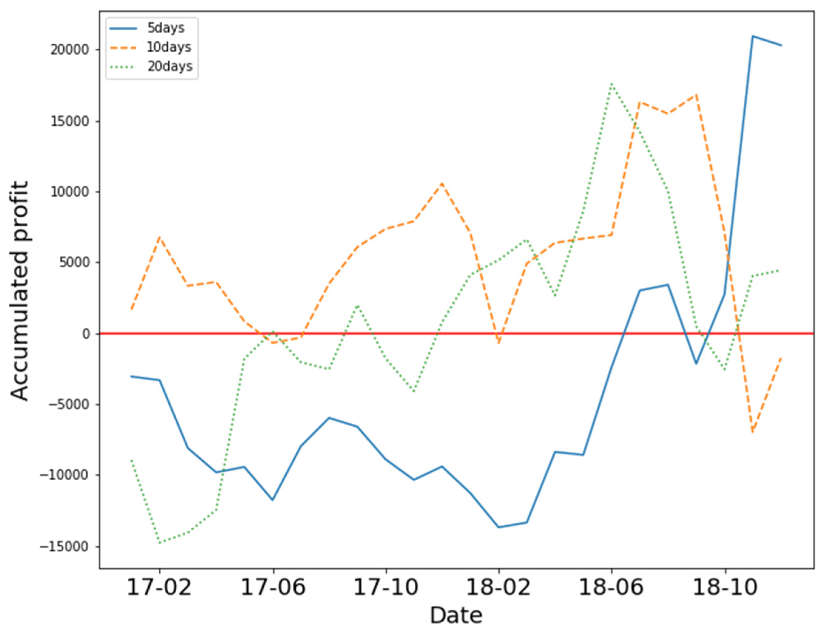
In Figure 4, the results show that 5-day, 10-day and 20-daysstates yielded positive profit. Training the model with 10 days of OHCLV on 1101 yielded the best performance. In addition, the model suffered a large loss in June 2018.

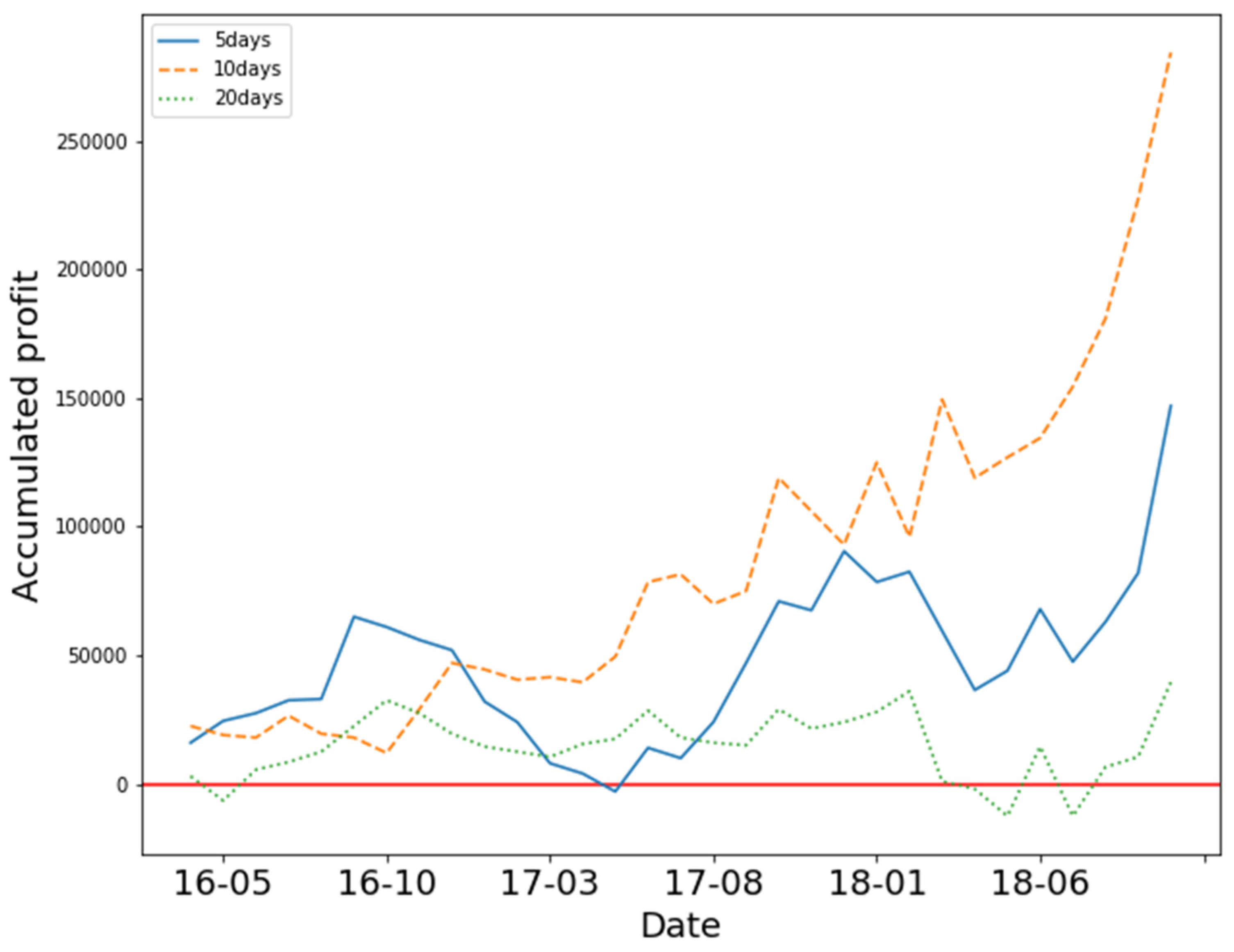
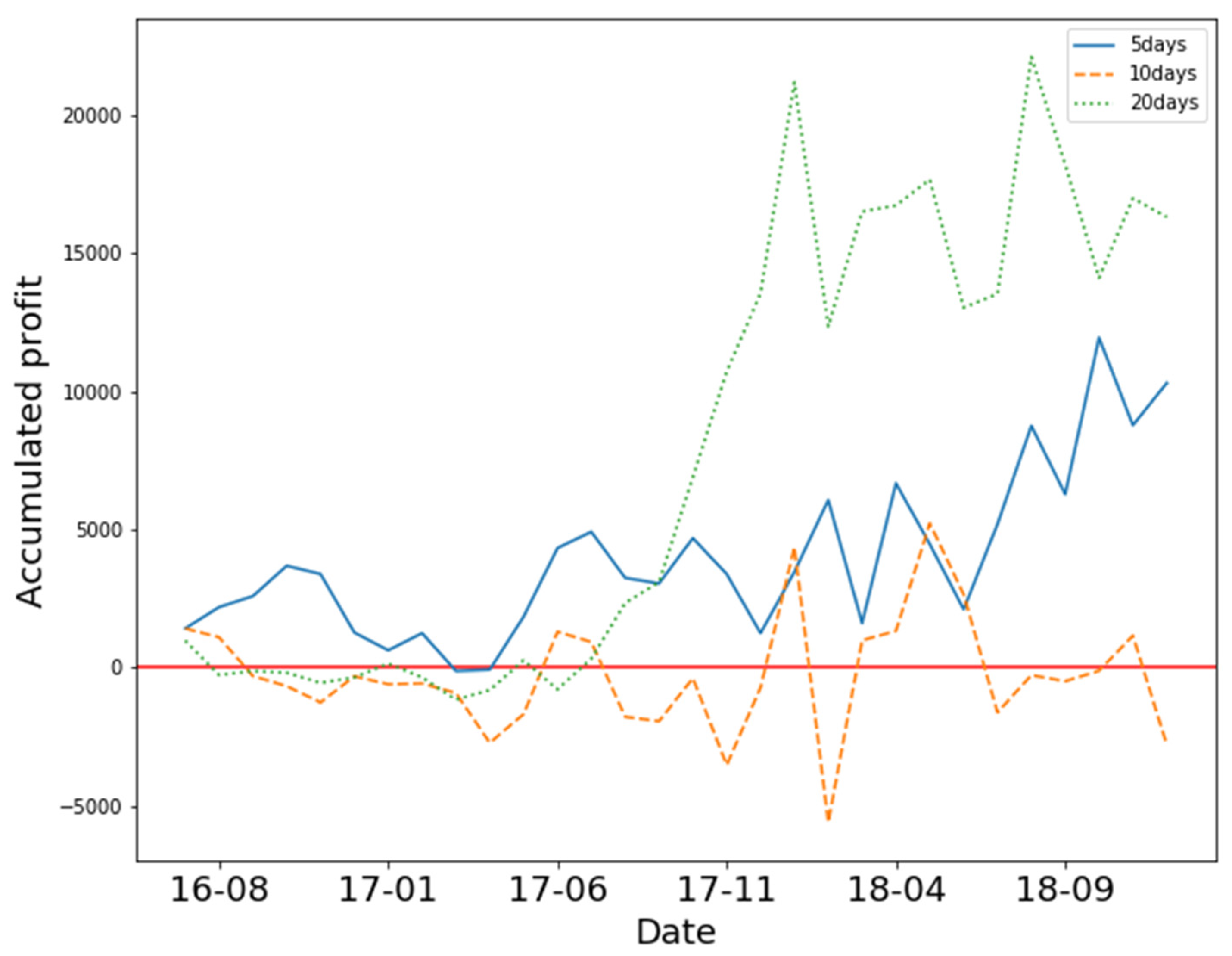
In Figure 5, the results show that all three states yielded positive profits over time. Training the model with 10 days of OHCLV on 2330 yielded the best performance.

In Figure 6, the results show that 10-day and 20-day states yielded positive profit, and the 5-day state yielded negative profit. Training the model with 10 and 20 days of OHCLV on 2881 yielded the best performance. The model for the 5-day state suffered a large loss in November 2016.

In Figure 7 and Figure 8, we trained the model to trade leveraged ETFs. Again, the Y axis represents accumulated profit, the X axis represents time, and the three different lines represent the accumulated profit of the three different states. Figure 7 shows that 5-day and 20-day states yielded positive profit. Figure 8 shows that the model suffered a large loss in November 2018.

As shown in

Table 4. Win rate.

Code	5 Days	10 Days	20 Days
0050	0.6035	0.4563	0.5357
1101	0.5102	0.5585	0.5760
2330	0.5580	0.5232	0.86
2881	0.5573	0.5398	0.5601
00655L	0.56034	0.4563	0.5357
00672L	0.48621	0.5212	0.5419

, we further used the win rate to analyze the performance of the framework. Our trading system’s win rates ranged between 48% and 60%; these low results were due to the goal of our framework, which was to build a framework that learns to trade a high stock spread between two days. The result show that our goal was achieved. Although we did not have a high win rate, we made a good profit.

4.3. The Evaluation of Financial Performance

The development of a strategy requires a good evaluation metric to judge whether the strategy is profitable. The most basic metrics include winning probability, odds ratio, maximum draw-down (MDD), and reward over MDD. We have listed the performance of our experiments in

Table 5. Evaluation metric of stock 2330.

	Maximum Draw-Down			Return over Maximum Draw-Down			Profit Factor
	5	10	20	5	10	20	5	10	20
	0.00%	0.00%	0.00%	mdd = 0	mdd = 0	mdd = 0	no loss	no loss	no loss
2016/4/1	0.00%	0.00%	0.00%	mdd = 0	mdd = 0	mdd = 0	no loss	no loss	no loss
2016/5/1	0.00%	−0.34%	−0.95%	mdd = 0	5.55	−0.69	no loss	6.43	0.32
2016/6/1	0.00%	−0.44%	−0.95%	mdd = 0	4.09	0.58	no loss	5.00	1.58
2016/7/1	0.00%	−0.44%	−0.95%	mdd = 0	6.02	0.90	no loss	6.89	1.89
2016/8/1	0.00%	−0.68%	−0.95%	mdd = 0	2.86	1.32	no loss	2.70	2.32
2016/9/1	0.00%	−0.83%	−0.95%	mdd = 0	2.17	2.38	no loss	2.38	3.37
2016/10/1	−0.38%	−1.41%	−0.95%	16.24	0.85	3.43	16.25	1.63	4.42
2016/11/1	−0.85%	−1.41%	−0.95%	6.63	2.05	2.90	7.22	2.53	2.90
2016/12/1	−1.22%	−1.41%	−1.26%	4.26	3.33	1.55	5.00	3.47	1.87
2017/1/1	−3.10%	−1.41%	−1.74%	1.03	3.15	0.83	1.97	3.07	1.53
2017/2/1	−3.85%	−1.41%	−1.94%	0.62	2.87	0.65	1.59	2.59	1.42
2017/3/1	−5.35%	−1.41%	−2.13%	0.15	2.94	0.49	1.14	2.63	1.33
2017/4/1	−5.73%	−1.41%	−2.13%	0.07	2.80	0.73	1.07	2.44	1.49
2017/5/1	−6.38%	−1.41%	−2.13%	−0.05	3.50	0.82	0.96	2.80	1.56
2017/6/1	−6.38%	−1.41%	−2.13%	0.22	5.56	1.34	1.21	3.85	1.90
2017/7/1	−6.38%	−1.41%	−2.13%	0.16	5.77	0.84	1.14	3.96	1.43
2017/8/1	−6.38%	−1.41%	−2.13%	0.38	4.96	0.75	1.33	2.79	1.36
2017/9/1	−6.38%	−1.41%	−2.13%	0.74	5.31	0.70	1.65	2.92	1.33
2017/10/1	−6.38%	−1.41%	−2.13%	1.11	8.42	1.36	1.99	4.05	1.64
2017/11/1	−6.38%	−1.41%	−2.13%	1.06	7.50	1.01	1.89	3.04	1.41
2017/12/1	−6.38%	−2.32%	−2.13%	1.42	4.00	1.13	2.20	2.43	1.46
2018/1/1	−6.38%	−2.32%	−2.13%	1.23	5.38	1.31	1.90	2.92	1.53
2018/2/1	−6.38%	−2.58%	−2.13%	1.29	3.72	1.69	1.94	2.02	1.69
2018/3/1	−6.38%	−2.58%	−3.38%	0.93	5.80	0.03	1.54	2.59	1.01
2018/4/1	−6.38%	−2.65%	−3.67%	0.57	4.48	−0.05	1.27	1.96	0.98
2018/5/1	−6.38%	−2.65%	−4.68%	0.69	4.79	−0.27	1.33	2.02	0.88
2018/6/1	−6.38%	−2.65%	−4.68%	1.07	5.07	0.31	1.51	2.08	1.14
2018/7/1	−6.38%	−2.65%	−4.68%	0.74	5.82	−0.27	1.31	2.24	0.90
2018/8/1	−6.38%	−2.65%	−4.68%	0.99	6.82	0.14	1.41	2.45	1.05
2018/9/1	−6.38%	−2.65%	−4.68%	1.28	8.57	0.22	1.53	2.83	1.08
2018/10/1	−6.38%	−2.65%	−4.68%	2.30	10.72	0.84	1.95	3.29	1.31

,

Table 6. Evaluation metric of stock 2881.

	Maximum Draw-Down			Return over Maximum Draw-Down			Profit Factor
	5	10	20	5	10	20	5	10	20
	0.00%	0.00%	0.00%	mdd = 0	mdd = 0	mdd = 0	no loss	no loss	no loss
2016/4/1	−0.29%	−0.31%	−0.26%	−1.00	−1.00	−1.00	0.00	0.00	0.00
2016/5/1	−0.29%	−0.31%	−0.26%	−0.34	−0.90	−0.54	0.66	0.10	0.46
2016/6/1	−0.29%	−0.31%	−0.26%	1.10	0.81	−0.04	2.10	1.81	0.96
2016/7/1	−0.29%	−0.31%	−0.26%	1.93	0.73	0.92	2.93	1.67	1.92
2016/8/1	−0.29%	−0.31%	−0.26%	2.78	1.24	1.63	3.78	2.15	2.63
2016/9/1	−0.44%	−0.31%	−0.37%	0.87	0.55	0.15	1.52	1.31	1.09
2016/10/1	−0.44%	−0.31%	−0.40%	1.05	0.81	0.05	1.63	1.45	1.03
2016/11/1	−1.10%	−0.31%	−0.40%	−0.26	1.10	2.21	0.80	1.62	2.34
2016/12/1	−1.41%	−0.31%	−0.40%	−0.43	1.44	2.80	0.66	1.81	2.70
2017/1/1	−1.43%	−0.31%	−0.40%	−0.44	1.18	2.41	0.66	1.58	2.18
2017/2/1	−1.46%	−0.31%	−0.40%	−0.45	1.56	2.70	0.65	1.77	2.32
2017/3/1	−1.46%	−0.31%	−0.40%	−0.37	2.03	2.42	0.71	2.00	2.04
2017/4/1	−1.66%	−0.38%	−0.40%	−0.51	0.64	2.74	0.61	1.24	2.18
2017/5/1	−1.75%	−0.41%	−0.40%	−0.54	0.52	2.48	0.58	1.21	1.96
2017/6/1	−1.75%	−0.44%	−0.40%	−0.53	0.42	2.59	0.59	1.17	2.00
2017/7/1	−1.75%	−0.51%	−0.40%	−0.52	0.24	2.94	0.59	1.11	2.13
2017/8/1	−1.75%	−0.55%	−0.40%	−0.49	0.15	2.74	0.62	1.07	1.98
2017/9/1	−1.75%	−0.59%	−0.40%	−0.54	0.07	3.14	0.60	1.03	2.12
2017/10/1	−1.82%	−0.67%	−0.40%	−0.56	−0.06	3.19	0.58	0.97	2.14
2017/11/1	−1.82%	−0.67%	−0.40%	−0.54	0.12	4.15	0.59	1.06	2.49
2017/12/1	−1.82%	−0.67%	−0.40%	−0.41	0.24	4.03	0.69	1.12	2.38
2018/1/1	−1.82%	−0.67%	−0.40%	−0.33	0.26	3.71	0.75	1.13	2.15
2018/2/1	−1.82%	−0.67%	−0.42%	−0.19	0.86	2.94	0.86	1.44	1.80
2018/3/1	−1.82%	−0.67%	−0.42%	−0.09	1.13	2.94	0.93	1.58	1.80
2018/4/1	−1.82%	−0.67%	−0.56%	−0.07	1.46	2.00	0.94	1.75	1.66
2018/5/1	−1.82%	−0.67%	−0.56%	−0.11	1.67	2.56	0.92	1.86	1.84
2018/6/1	−1.82%	−0.67%	−0.93%	−0.36	1.09	0.79	0.78	1.43	1.31
2018/7/1	−1.82%	−0.67%	−0.93%	−0.32	1.18	0.85	0.80	1.46	1.33
2018/8/1	−1.82%	−0.67%	−0.95%	−0.43	1.06	0.74	0.75	1.40	1.29
2018/9/1	−1.82%	−0.67%	−0.95%	−0.46	1.17	0.85	0.74	1.44	1.33
2018/10/1	−1.82%	−0.67%	−1.04%	−0.22	0.83	0.60	0.88	1.28	1.23

,

Table 7. Evaluation metric of stock 0050.

	Maximum Draw-Down			Return over Maximum Draw-Down			Profit Factor
	5	10	20	5	10	20	5	10	20
	0	0	0	mdd = 0	mdd = 0	mdd = 0	no loss	no loss	no loss
2016/4/1	0.00%	0.00%	−0.05%	mdd = 0	mdd = 0	−1.00	no loss	no loss	no loss
2016/5/1	−0.29%	−0.06%	−0.05%	−0.35	−1.00	10.00	0.66	0.00	11.00
2016/6/1	−0.46%	−0.06%	−0.45%	−0.59	−0.67	0.11	0.41	0.33	1.10
2016/7/1	−0.62%	−0.20%	−0.45%	−0.69	−1.00	1.12	0.31	0.09	2.00
2016/8/1	−0.87%	−0.20%	−0.45%	−0.78	−0.10	3.35	0.22	0.91	4.00
2016/9/1	−1.36%	−0.20%	−0.45%	−0.86	−0.15	2.90	0.14	0.87	2.86
2016/10/1	−1.36%	−0.20%	−0.45%	−0.69	−0.90	2.68	0.32	0.53	2.50
2016/11/1	−1.36%	−0.20%	−0.45%	−0.35	−0.85	3.91	0.65	0.55	3.19
2016/12/1	−1.36%	−0.20%	−0.45%	−0.21	−0.55	3.80	0.79	0.71	3.00
2017/1/1	−1.36%	−0.20%	−0.45%	−0.21	−1.00	4.02	0.79	0.57	3.12
2017/2/1	−1.36%	−0.20%	−0.45%	0.27	−0.50	4.02	1.26	0.79	3.12
2017/3/1	−1.36%	−0.20%	−0.45%	0.41	−0.52	3.91	1.40	0.78	2.94
2017/4/1	−1.36%	−0.20%	−0.45%	0.45	−0.67	4.80	1.45	0.73	3.39
2017/5/1	−1.36%	−0.20%	−0.45%	0.48	−0.97	4.24	1.48	0.65	2.65
2017/6/1	−1.36%	−0.21%	−0.45%	0.52	−1.00	3.91	1.51	0.63	2.35
2017/7/1	−1.36%	−0.27%	−1.13%	0.17	−1.00	0.89	1.13	0.58	1.49
2017/8/1	−1.36%	−0.28%	−1.13%	0.24	−1.00	1.20	1.17	0.57	1.66
2017/9/1	−1.36%	−0.33%	−1.32%	0.22	−1.00	0.61	1.16	0.52	1.31
2017/10/1	−1.36%	−0.41%	−1.32%	0.18	−1.00	1.06	1.13	0.47	1.54
2017/11/1	−1.36%	−0.44%	−1.91%	0.26	−1.00	0.10	1.18	0.45	1.05
2017/12/1	−1.36%	−0.47%	−1.91%	0.28	−1.00	0.13	1.20	0.44	1.07
2018/1/1	−1.36%	−0.56%	−1.91%	0.25	−1.00	0.84	1.17	0.40	1.42
2018/2/1	−1.36%	−0.56%	−1.91%	0.65	−0.96	1.26	1.45	0.42	1.63
2018/3/1	−1.36%	−0.75%	−1.91%	0.52	−1.00	2.10	1.33	0.34	2.05
2018/4/1	−1.36%	−0.75%	−1.91%	0.40	−0.97	1.70	1.24	0.36	1.71
2018/5/1	−1.36%	−0.75%	−1.91%	1.04	−0.60	1.70	1.62	0.60	1.71
2018/6/1	−1.36%	−0.75%	−1.91%	1.27	−0.44	1.70	1.75	0.71	1.71
2018/7/1	−1.36%	−0.75%	−1.91%	2.19	−0.53	1.15	2.30	0.67	1.39
2018/8/1	−1.36%	−0.75%	−2.79%	2.31	−0.52	0.39	2.37	0.68	1.16
2018/9/1	−1.36%	−0.75%	−2.79%	2.48	−0.19	0.63	2.47	0.88	1.26
2018/10/1	−1.36%	−0.75%	−2.79%	1.84	−0.34	0.97	1.79	0.80	1.40

and

Table 8. Evaluation metric of stock 1101.

	5	10	20	5	10	20	5	10	20
	0.00%	0.00%	0.00%	mdd = 0	mdd = 0	mdd = 0	no loss	no loss	no loss
2016/4/1	−0.14%	0.00%	0.00%	−1.00	mdd = 0	mdd = 0	0.00	no loss	no loss
2016/5/1	−0.14%	0.00%	−0.02%	0.15	mdd = 0	6.51	1.15	no loss	7.50
2016/6/1	−0.19%	−0.04%	−0.02%	−0.89	4.51	7.51	0.48	5.50	8.50
2016/7/1	−0.19%	−0.26%	−0.02%	0.61	−0.15	9.01	1.35	0.85	10.00
2016/8/1	−0.19%	−0.26%	−0.17%	0.71	0.73	0.06	1.42	1.73	1.05
2016/9/1	−0.19%	−0.26%	−0.17%	1.18	0.46	1.59	1.69	1.36	2.42
2016/10/1	−0.19%	−0.26%	−0.17%	1.13	0.35	1.77	1.64	1.25	2.58
2016/11/1	−0.19%	−0.26%	−0.17%	1.47	0.19	1.24	1.84	1.13	1.75
2016/12/1	−0.19%	−0.26%	−0.17%	1.42	0.27	1.59	1.78	1.18	1.96
2017/1/1	−0.19%	−0.26%	−0.23%	0.74	−0.15	0.31	1.29	0.92	1.15
2017/2/1	−0.19%	−0.30%	−0.30%	3.40	−0.27	−0.02	2.36	0.85	0.99
2017/3/1	−0.19%	−0.30%	−0.43%	3.50	0.53	−0.30	2.40	1.29	0.81
2017/4/1	−0.19%	−0.30%	−0.43%	4.13	0.37	−0.12	2.65	1.18	0.93
2017/5/1	−0.25%	−0.30%	−0.43%	2.09	0.03	−0.24	1.73	1.01	0.86
2017/6/1	−0.26%	−0.30%	−0.43%	1.98	0.07	−0.28	1.70	1.03	0.84
2017/7/1	−0.26%	−0.39%	−0.43%	2.72	−0.44	−0.03	1.97	0.81	0.98
2017/8/1	−0.26%	−0.40%	−0.43%	2.28	−0.45	−0.29	1.70	0.80	0.85
2017/9/1	−0.26%	−0.40%	−0.52%	2.17	−0.35	−0.43	1.64	0.84	0.77
2017/10/1	−0.26%	−0.40%	−0.57%	2.17	−0.43	−0.48	1.64	0.82	0.73
2017/11/1	−0.27%	−0.40%	−0.57%	1.92	−0.43	−0.46	1.55	0.82	0.74
2017/12/1	−0.31%	−0.40%	−0.65%	1.50	−0.18	−0.54	1.48	0.92	0.68
2018/1/1	−0.31%	−0.40%	−0.65%	1.50	0.13	−0.22	1.48	1.05	0.87
2018/2/1	−0.31%	−0.40%	−0.65%	1.65	0.13	−0.15	1.52	1.05	0.91
2018/3/1	−0.34%	−0.40%	−0.65%	1.32	−0.14	−0.28	1.42	0.95	0.85
2018/4/1	−0.34%	−0.40%	−0.65%	1.42	0.29	0.11	1.45	1.11	1.06
2018/5/1	−0.34%	−0.40%	−0.65%	4.21	0.51	2.10	2.35	1.20	2.16
2018/6/1	−0.34%	−0.40%	−0.65%	4.94	0.84	1.69	2.58	1.32	1.76
2018/7/1	−0.91%	−0.40%	−1.28%	0.80	3.60	0.05	1.37	2.39	1.03
2018/8/1	−1.03%	−0.40%	−1.28%	0.60	4.47	0.38	1.29	2.72	1.19
2018/9/1	−1.03%	−0.40%	−1.28%	0.76	5.10	0.18	1.38	2.97	1.08
2018/10/1	−1.21%	−0.40%	−1.28%	0.35	4.45	0.27	1.17	2.37	1.13

. In terms of profit factor (PF), if it is greater than 1, the strategy is in a profitable state. Generally, PF is recommended to be greater than 1.5, so that the cumulative profit and loss curve rises steadily. In the experiment, we observed that our trading model performed well for most parameters.

5. Conclusions and Future Work

Traditionally, it is difficult to create a trading strategy. We must analyze many aspects of the target—price data, technical indicators, and so on—after which we must decide when to trade and how many shares to trade. This is a difficult and time-consuming job for traders. Hence, we built an automated trading framework based on deep neural networks and reinforcement learning. The experiment used five different Taiwan stock constituents from January 2009 to December 2018.

We make three key contributions to the literature: focusing on the different deep neural networks, we found that LSTM outperformed other neural networks in financial time series prediction tasks based on our collected stock data. LSTM outperformed for four of five different stocks. The second contribution is our automated trading system, based on five kinds of basic daily price data (e.g., open price, highest price, closed price, lowest price, and volume). Our trading strategy was daily trading within two days. We obtained trading signals and sizes from our framework to decide whether to sell, hold or buy, and close the position the next day. We demonstrated that the proposed framework yielded good returns in some stocks. However, we only verified our framework on the Taiwan stock market, and we used the same neural network to construct a framework for five different stocks.

Recently, some researchers have proposed framework integrated stock prices and financial news for stock prediction. In future research, sentiment analysis of news articles should be integrated as another resource of information on the environment. A reinforcement learning model should also be applied in the cryptocurrency market, including Bitcoin, Ethereum, and so on.

A limitation is that the proposed model was only evaluated for one stock at the Taiwan stock market. Since we were limited with respect to funding, we only collected a small dataset for evaluating the proposed model. Future work should include verifying the proposed model by collecting a larger dataset.