The implementation of the neural networks for modeling the separation cascade dynamics is justified due to the following three aspects:
2. The possibility to implement an online adaption algorithm for some of the neural network’s parameters, in order to adapt the proposed model at the physical variations of the separation cascade structure parameters;
3. The possibility to use neural networks for the future intelligent control of the separation cascade and to apply the same training algorithm as in the case of the proposed model.
4.1. Proof of Neural Model Higher Accuracy
In order to highlight the mentioned advantages, two other types of models (the polynomial models and the Spline type models) are comparatively studied with the proposed neural model.
(1) The polynomial approximating functions.
The polynomial approximating function’s general form is given by:
where
n is its degree and
pi (
i {0, 1, 2, 3, …,
n}) are its coefficients. Moreover, the polynomial approximating function variable is denoted by
z. The approximation of a certain function using the polynomial function consists of determining (identifying) the values of the
pi (
i {0, 1, 2, 3, …,
n}) coefficients in order to obtain the best fit between the two functions. The limitations of the polynomial approximation can be easily highlighted in the cases of the
SFST(
Ff) and the
SPST(
Fi) functions. By varying the polynomial degree, it its observed that the fitting quality of the results is varying too. Consequently, a study regarding the polynomial degree influence over the approximation accuracy is carried on. In the case of the
SFST(
Ff) function, 1251 samples were considered in order to be processed with the purpose of obtaining the polynomial approximating functions. By using these samples and applying the Least Square Method [
66], three polynomial approximating functions are determined, having the degrees:
n1 = 10,
n2 = 20 and
n3 = 50. The comparative graph between the real form of the
SFST(
Ff) function and the responses of the three obtained polynomial approximating functions is presented in
Figure 5.
From
Figure 5, a low accuracy of the polynomial approximating functions in modeling the
SFST(
Ff) function, results.
This conclusion is obvious since between the three polynomial responses and the
SFST(
Ff) function, a consistent difference in values on certain domains of F
f signal values can be observed (the most consistent variations occur in the neighborhood of the
Ffc value). Another important aspect is referring to the fact that if we increase the degree of the polynomial approximating function, in the domain of F
f high values (in the neighborhood of
Ffmax; this domain is highlighted on the right part of
Figure 5 with a circle), the corresponding response presents oscillations. The higher the polynomial approximating function degree, the higher its response oscillations. Consequently, a lower fit between the polynomial function response and the
SFST(
Ff) function will be obtained for high values of
Ff and implicitly (as error) for the entire range of
Ff values. The low quality of the polynomial identification can be also highlighted through the MSE values obtained between the responses of the three polynomials presented in
Figure 5 and the response of
SFST(
Ff) function, values centralized in
Table 5.
All the MSE values from
Table 5 are computed on 1251 pairs of samples of
SFST(
Ff) function response and of each polynomial response. In the last column of
Table 5, the MSE value associated to a 100th degree polynomial approximating function (for the
SFST(
Ff) function) is presented. From
Table 5, the result is that increasing the degree of the polynomial approximating function until the value of 50, the approximation accuracy increases, but after this value, the approximation accuracy starts to decrease. The explanation of this phenomenon is given by the following: the oscillations occurrence in the domain of F
f signal high values, for the polynomials with higher degrees; the oscillations’ amplitude increases at the polynomial degree increase. In this context, it can be remarked that the MSE value is higher in the case of using the 100th degree polynomial than in the case of the 50th degree polynomial. Consequently, the final solution for the
SFST(
Ff) function approximation using polynomial functions is obtained using a 50th degree polynomial.
However, by comparing the neural approximation accuracy with the 50th degree polynomial approximation accuracy, the neural model can be observed to be much more accurate.
The better performances generated by the proposed neural model are proven by the MSE values: the value of MSE computed in the case of the neural model, presented in
Table 4 (
MSE = 5.73∙10
−4) is much lower (of more than 100 times) than the lowest value presented in
Table 5 (
MSE = 2.2∙10
−2; generated by the 50th degree polynomial approximating function).
In the case of the SPST(Fi) function, the polynomial approximating functions are determined, too. After applying the same procedure as in the case of SFST(Ff) function and considering the same degrees for the polynomials (n1 = 10, n2 = 20 and n3 = 50), the same conclusions as in the case of SFST(Ff) function, results.
The MSE values between the responses of the three polynomials and the real response of
SPST(
Fi) function are computed on 1251 pairs of samples of
SPST(
Ff) function response and of each polynomial response. These values are centralized in
Table 6.
Consequently, the same conclusion that the proposed neural model is much more accurate, results. This conclusion is confirmed, also, by the consistent difference between the MSE values (in the case of the neural model, the value MSE = 7.91∙10
−4 is obtained (
Table 5), which is lower (almost of 100 times) than the lowest value from
Table 6 (MSE = 0.0605 obtained for the 50th degree polynomial).
In order to compare the effects of the two types of the approximations (neural and polynomial) accuracies, the comparative graph from
Figure 6 is presented. In
Figure 6, the most probable response of the separation cascade is comparatively presented with the separation cascade models responses obtained by using the neural and the polynomial approximation types (for the same simulation, both the
SPST(
Fi) and the
SFST(
Ff) functions are approximated using the same approximation type).
The simulations from
Figure 6 are performed for the input flows
Fi =
Fic = 1785.71 L/h (in the PSC) and
Ff =
Ffc = 140 L/h (in the FSC), for which the errors between the theoretical forms of the
SPST(
Fi), respectively, the
SFST(
Ff) functions and the responses of the two types of their approximations (neural and polynomial) are maximum. For the three cases, the values of the
SPST(
Fic) and the
SFST(
Ffc) functions are centralized in
Table 7. For both functions, the values deviations of the neural approximations in relations to the theoretical values (Δ
SPST(
Fic) = 0.0265 and Δ
SFST(
Ffc) = 0.0166) are much smaller than the values deviations of the polynomial approximations in relations to the theoretical values (Δ
SPST(
Fic) = 0.4332 and Δ
SFST(
Ffc) = 0.125).
This aspect implies a much better accuracy generated by the neural model in comparison to the polynomial model. Analyzing
Figure 6, a much better superposition of the response generated by the separation process model (over the most probable response) can be remarked in the case when the
SPST(
Fi) and the
SFST(
Ff) functions are approximated using neural networks than in the case when they are approximated using polynomial functions. The better accuracy obtained by using the neural approximations is proven through the MSE values computed (on 3001 pairs of samples considering the sampling time Δ
TS = 1 h) between the responses from
Figure 6. Consequently, using the values of the red and of the blue curves from
Figure 6, the error
MSE = 0.0793% is computed. This error is much smaller than the
MSE = 0.9215% error computed between the values of the green and of the blue curves from
Figure 6.
In conclusion, by using the neural approximation of the SPST(Fi) and the SFST(Ff) functions, we obtain an accurate model of the separation cascade operation, but in the case of the polynomial approximation, we obtain an unacceptable accuracy (an MSE value equal to 0.9215%, and a deviation of the cascade response in steady-state regime of 1% are considered “huge” deviations for the isotope separation applications).
An interesting comparison between different types of approximations can be made referring to their number of coefficients. In the case of the 50th degree polynomial approximation, 51 coefficients are used, according to (21) (pi (i {0, 1, 2, 3, …, 50})). In the case of the neural approximation, a total of 108 weights and bias values are used, but they are approximating 3 functions in the same time (for example, considering NNPSC, it approximates the SPST(Fi), T1(Fi) and R1(Fi) functions).
Hence, the result is that for each function, an average of 36 (the third part from 108) parameters are used.
For each obtained neural solution (having 21 nonlinear neurons in the hidden layer and 3 linear neurons in the output layer), the total of 108 can be split in: 21 input weights + 63 (3·21) weights between the hidden and the output layer + 21 bias values of the neurons from the hidden layer + 3 bias values for the neurons of the output layer. Taking in account all the conclusions above, using the neural approximation, we obtain a better accuracy than in the case of using the polynomial approximation and, at the same time, with less model parameters (36 < 51).
Another type of approximation that was considered is the interpolation Spline function. In contrast to the polynomial approximation functions, in the case of the interpolation Splines, the variation domain of the input variable (signal) is decomposed in a certain number of subdomains, each subdomain being bounded by two consecutive interpolation points. If we preserve the general notation of the variable from (21), then an example of a subdomain is [
zi,
zi+1], where
zi and
zi+1 are two consecutive interpolation points and
i {1, 2, 3, ……,
n − 1}, where
n represents the total number of the considered interpolation points (the
n value is restricted by the number of the available interpolation points or, if there are available a consistent number of interpolation points, the
n value can be imposed in order to limit the total number of the interpolation Spline parameters). For the considered technical application, the case of the Cubic interpolation Spline function is considered. Consequently, the variation form of the approximated function, on each resulted subdomain [
zi,
zi+1], is estimated using the Cubic interpolation Spline from (22):
where
i {1, 2, 3, ……,
n − 1}. For each subdomain (subinterval) the
ai,
bi,
ci and
di can be determined using the natural cubic spline method [
53]. The notation
fi =
f(
zi) is used for the approximated function value for the input variable values
zi (
i {1, 2, 3, ……,
n − 1}), values which are known.
Then, the approximation of the SPST(Fi) and the SFST(Ff) functions, using the Cubic interpolation Spline is presented. In order to obtain a similar number of parameters of the interpolation Spline function (cumulated on all subintervals) with the parameters of the proposed neural approximation, a number of 26 interpolation points are considered. Consequently, 25 subintervals of the Fi and Ff input signals result. As a remark, the considered interpolation points are considered equidistant. It results that the total number of parameters of each from the two interpolation Spline functions, which are used for the approximation of the SPST(Fi) and the SFST(Ff) functions, is 100 (4 parameters ai, bi, ci and di for each of the 25 subintervals).
In the case of the
Ff input signal, 26 interpolation points are considered, starting with the lowest possible value of 60 L/h and maintaining the step Δ
Ff = 5 L/h (hence, including the highest possible value of 185 L/h). After applying the natural cubic spline method and finding for all 25 intervals the
ai,
bi,
ci, and
di coefficients, the comparative graph from
Figure 7 can be presented.
From
Figure 7, we notice that the response generated by the Spline type approximating solution presents visible deviations in relation to the other two responses, aspect which implies its lower accuracy. The same conclusion is obtained as a result of the
SPST(
Fi) function variation. In
Figure 7, the interval of the responses in which the most consistent deviation between the response of the Spline type approximation and the real form of
SFST(
Ff) function, is highlighted using the circle. The lower quality of the Spline type approximation can be also proven through the values of the Mean Square Errors between the values of the
SFST(
Ff) respectively, of the
SPST(
Fi) functions and the values of the responses of the associated Spline type, respectively, neural approximations. In
Table 8, the centralizer containing the computed MSE values is presented. In order to compute the MSE for 1251 pairs of values, the same samples of the
SPST(
Fi) and the
SFST(
Ff) functions are used as in the case of the polynomial approximation. Consequently, the MSE values associated to the neural approximation (computed for 1251 pairs of values) are presented in
Table 5, as well. In the case of computing the MSE for 25 pairs of values, the 25 subintervals associated to the procedure of determining the Spline type approximation, are considered.
In the case of each function
SPST(
Fi), respectively,
SFST(
Ff) and in the case of all associated approximating functions (neural and Spline types), for the MSE computation, their values at the center of each subinterval are considered (the centers of the 25 intervals are considered in relation to
Fi and
Ff input signals; in the case of the general notation, the center of each subinterval is the average value
zav = (
zi +
zi+1)/2). This aspect is due to the fact that, for the Spline approximation, the accuracy cannot be highlighted by computing the MSE in the interpolation points, because it would result in the value
MSE = 0. This is because in (22),
di =
fi (
i {1, 2, 3, ……,
n − 1}). Obviously, the
MSE = 0 value is not a realistic one after analyzing
Figure 7.
From
Table 8, it results that in both the
SPST(
Fi) and the
SFST(
Ff) functions and for both two methods of computing MSE, the neural approximation generates a much better accuracy. Moreover, from
Figure 7, it results that the highest error between the
SFST(
Ff) function and the associated Spline type approximation occurs for
Ff = 141.9 L/h, having the value
E2 = 0.096 (absolute value). Considering these values of the input signals (
Fi = 1807.4 L/h and
Ff = 141.9 L/h), the comparative graph between the most probable response of the separation cascade and the responses of the separation cascade models using the Neural Networks, respectively, the Spline types of approximation (simultaneously, for both
SPST(
Fi) and
SFST(
Ff) functions, the same approximation type is used), is presented in
Figure 8. In
Figure 8, it is obvious that, using the neural approximation for the
SPST(
Fi) and for the
SFST(
Ff) functions, the mathematical model of the separation cascade is much more precise than in the case of using the Spline type approximations (the dashed red curve is almost perfectly superposed over the continuous blue one; at the same time the green curve presents a consistent deviation in relation to the other two curves). This happens because, for
Fi = 1807.4 L/h and
Ff = 141.9 L/h, the errors between the
SPST(
Fi), respectively, the
SFST(
Ff) functions and the responses of their neural approximations are proportional with 10
−4. The better performance of the proposed neural models can be proven through the MSE values, too. Hence, 3001 pairs of samples of the curves from
Figure 8 are considered, by applying the same sampling time Δ
TS = 1 h as in the case of the simulations from
Figure 6. After computation, between the red and the blue curve from
Figure 8, the value
MSE = 0.0035% is obtained, which is much lower than the value
MSE = 0.6294% computed between the green and the blue curves from
Figure 8.
Consequently, the MSE obtained in the case of using the neural approximations is more than 100 times smaller than the MSE obtained in the case of Spline type approximations. Moreover, the error value of 0.0035% is considered to be insignificant for the isotope separation applications, but the error value of 0.6294% is a “huge” one for these types of applications and it is considered unacceptable. Additionally, in a steady-state regime, the deviation of the red curve in relation to the blue curve is only of 4 × 10⁻³% (an insignificant value), but the deviation of the green curve in relation to the blue curve is of 0.6631% (an unacceptable deviation).
In contrast to the polynomial type of approximation, if, in the case of the Spline function, the number of the interpolation points is consistently increased, the accuracy of the approximation can be significantly increased. Hence, in order to obtain approximately the same accuracy as in the case of using the neural solutions, the number of the interpolation points must be increased to 187. The main problem in this case is the fact that a total of 744 parameters of the Spline function result (4 parameters for each of 186 resulted subintervals), a value much higher than 36 (the average number of parameters of the neural solution used for modeling one of the 3 modeled functions).
Another important problem refers to the T1(Fi) and T2(Ff) functions approximation. These functions do not present a monotony change, an aspect which implies the fact that the approximation of their behavior is simpler than in the cases of the SPST(Fi) and the SFST(Ff) functions. Consequently, the polynomial approximation is tested and the T2(Ff) function is considered as a case study. In this context, a 25th degree polynomial with the structure presented in (21) is used, and the same procedure for determining the polynomial coefficients is applied.
The higher accuracy of the neural model is proven through the MSE values between the resulted responses. Hence, considering 1251 samples of the curves, the MSE obtained between the responses of the neural model and the identified function is 6.46∙10−5 h, and the MSE obtained between the responses of the polynomial model and the identified function curve is 8.48 × 10⁻⁵ h. It results that the neural model generates a sensible higher accuracy than the polynomial model. The same conclusion results in the case of the approximation of T1(Fi) function (using a 25th degree polynomial and the NNPSC). Consequently, in the cases of the T1(Fi) and T2(Ff) functions, considering the fact that the neural solutions generate sensible better solutions than the polynomial ones, but the polynomial approximations have a smaller number of parameters than the neural ones (each polynomial presents 26 coefficients, a smaller number than 36 average parameters of each neural solution), the usage of the two approximating models imply the same degree of advantage. In this context, the analysis of the Spline type approximation is no longer necessary.
In the case of the R1(Fi) and the R2(Ff) functions approximation, the problem is more complicated than in the case of the T1(Fi) and T2(Ff) functions approximation, because they present a monotony variation. In this context, the usage of the polynomial approximation is not efficient due to the same explanations as in the case of the SPST(Fi) and SFST(Ff) functions. Using the same procedure as in the case of the SPST(Fi) and SFST(Ff) functions, it can be proven that the neural approximation of the R1(Fi) and the R2(Ff) functions generates a consistent higher accuracy than the Spline type approximation. Considering the presented study, the following conclusions, which justify the neural network usage as modeling solution, result:
NNPSC and NNFSC represent unitary models, which (each) learn the behavior of three functions (simultaneously), by applying the Levenberg–Marquardt learning algorithm;
The accuracy generated by NNPSC and NNFSC is much higher in the case of learning the behavior of SPST(Fi), SFST(Ff), R1(Fi), and R2(Ff) functions, respectively, it is sensibly higher in the case of learning the behavior of T1(Fi) and T2(Ff) functions; this remark is valid comparing the two neural models with the polynomial, respectively, the Spline models;
The higher accuracy generated by NNPSC and NNFSC is obtained using much fewer parameters than in the cases of the polynomial and the Spline functions; hence, NNPSC and NNFSC each use 108 weights and bias values; it results in an average number of 36 parameters used for each function learning (both NNPSC and NNFSC learn 3 functions simultaneously);
The best solution of using the polynomial approximations implies the use of 128 parameters for modeling the group of functions (SPST(Fi); T1(Fi); R1(Fi)) and of other 128 for modeling the group of functions (SFST(Ff); T2(Ff); R2(Ff)); for example, in the case of the group of functions (SPST(Fi); T1(Fi); R1(Fi)), the polynomial that models the SPST(Fi) function contains 51 coefficients, the polynomial that models the T2(Ff) contains 26 coefficients, and the polynomial that models the R1(Fi) function contains 51 coefficients; the main problems of the polynomial models is the fact that they cannot model with an acceptable accuracy the SPST(Fi), SFST(Ff), R1(Fi) and R2(Ff) functions;
The sufficient solution for using the Spline functions, which generate approximately the same accuracy as NNPSC and NNFSC, imply the usage of 1644 parameters for modeling the group of functions (SPST(Fi); T1(Fi); R1(Fi)) and of other 1644 for modeling the group of functions (SFST(Ff); T2(Ff); R2(Ff)); for example, in the case of the group of functions (SPST(Fi); T1(Fi); R1(Fi)), the Spline function that models the SPST(Fi) function contains 744 coefficients, the Spline function that models the T2(Ff) contains 208 coefficients, and the Spline function that models the R1(Fi) function contains 692 coefficients; consequently, the main problem of the Spline functions is the extremely high number of coefficients that have to be used in order to generate the same accuracy as the neural models; hence, the numerical implementation of Spline functions is very difficult due to the large number of parameters and consequently the resulted large dimensions of the corresponding look-up tables;
The three types of approached methods of the approximation (neural, polynomial, and Spline type) were tested in the most unfavorable conditions; both on the entire range of input signals values and in the most unfavorable conditions, the neural networks generated the highest accuracy;
The most consistent advantage of using the neural approximations, from the accuracy perspective, is obtained for the learning of the SPST(Fi) and the SFST(Ff) functions; these two functions have the most important influence over the separation cascade model’s accuracy;
Considering all the above, we may conclude that the use of NNPSC and NNFSC is recommended in the separation cascade model, giving us the possibility of using the model in future control applications.
4.4. Strategies for the Adaptive Learning of the Separation Cascade Behavior
An important future research direction which will be approached soon is represented by the online identification of the separation cascade instantaneous mathematical model.
- (a)
Prove the feasibility of online adapting the proposed model.
During the operation, some of the structure parameters of the separation cascade can present variations in relation to time, resulting in the necessity of adapting the initial form of the proposed model. Next, the case of the variation of the parameters of the
HETP1(
Fi) function from (3) is presented (for example, HETP
1C, K
H10, or/and K
H20), a variation that has as an effect, the increase in this function and implicitly the decrease in the
SPST(
Fi) function. The online adapting of the proposed model to these possible variations can be made by using the Adaptive Mechanism from
Figure 9.
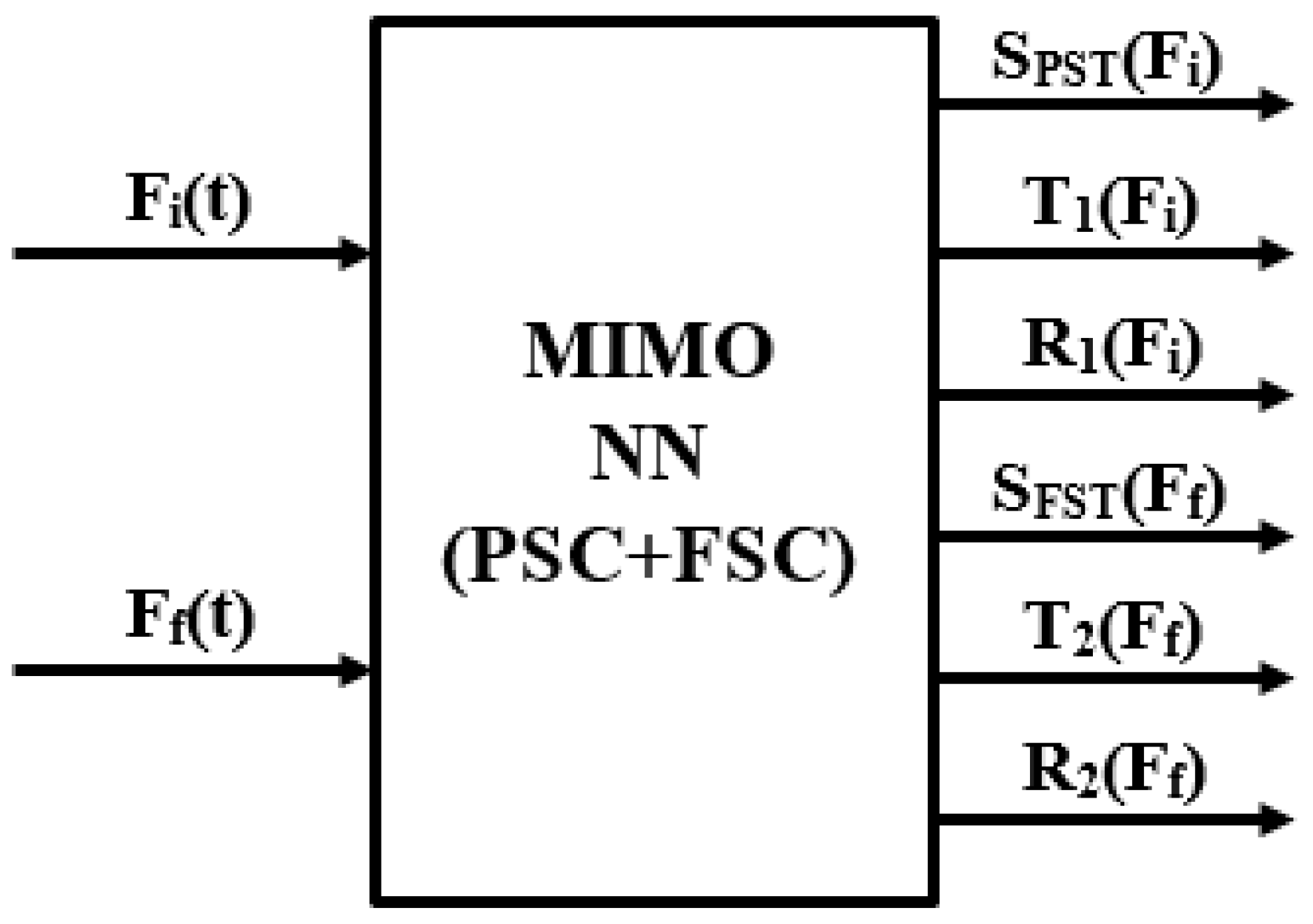
In
Figure 9, the proposed model based on the usage of the neural networks is run in parallel with the real separation process, the same input signals (
Fi) and (
Ff) being applied to the input of both entities. In this figure, the notation
xFR(
t,
r) is referring to the real concentration of the
18O isotope at the output from FSC, and the notation
xFS(
t,
r) is referring to the simulated concentration of the
18O isotope at the output from FSC, obtained by simulating the proposed mathematical model. The difference between the two signals gives the error signal
e(
t,
r). The error signal is applied at the input of the Adaptive Mechanism, which processes its value and generates the adaptation signal. Analyzing
Figure 2, the
SPST(
Fi) function approximation is generated by NNPSC at the output of the NO
PSC1 neuron, results. Consequently, a direct solution for adapting the proposed model to the variation of the mentioned structure parameters is to adapt the bias value of the NO
PSC1 neuron (
bOLPSC1). In this context, after processing the error value, the Adaptive Mechanism generates the adaptation signal (Δ
bOLPSC1), which is added to the initial (
bOLPSC1) bias value.
In the approached particular case, the Adaptive Mechanism is implemented by using a PI (Proportional Integral) controller.
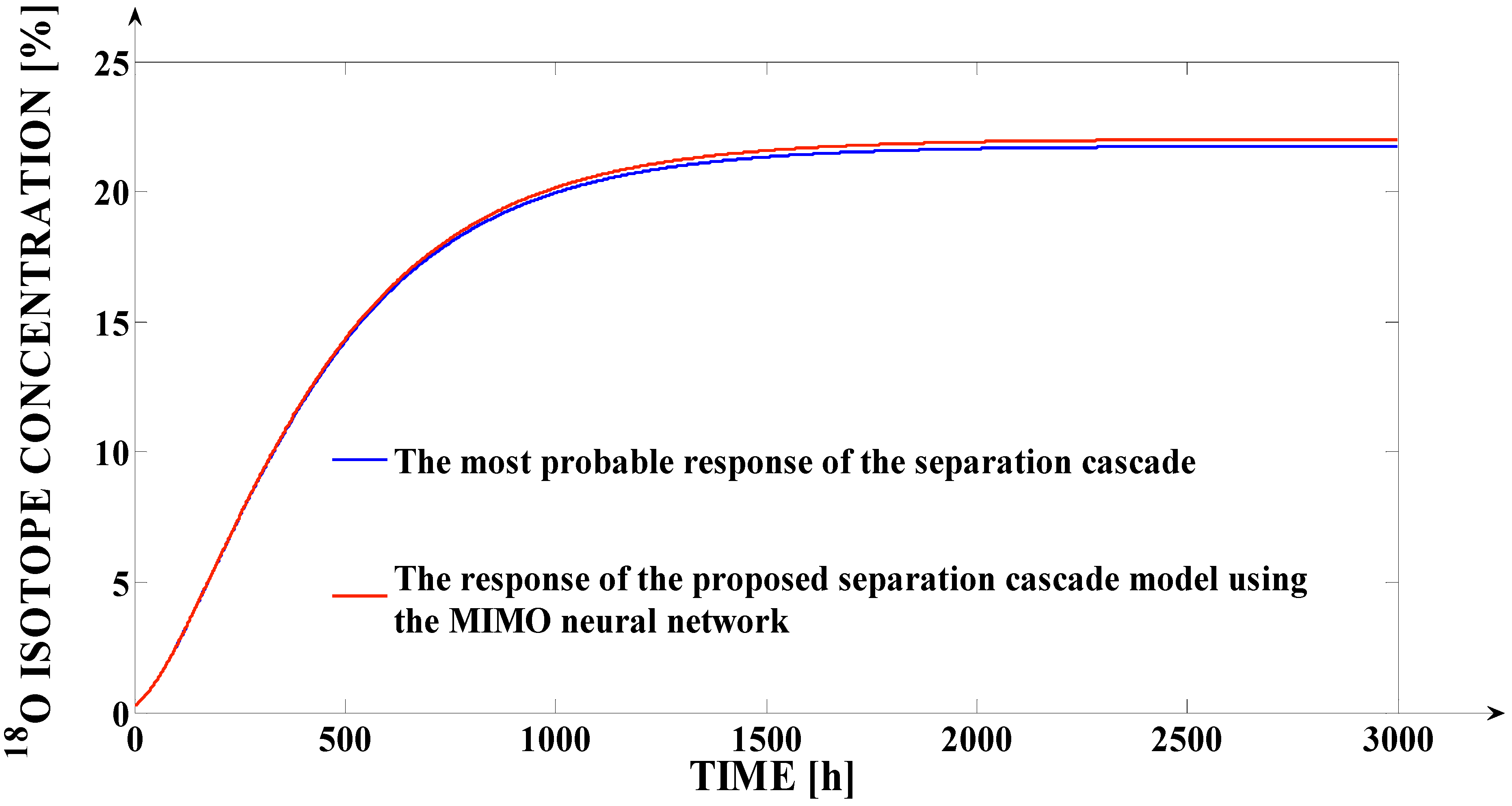
In
Figure 10, the effects of the variation of the mentioned structure parameters (which are due to some parametric disturbances) and of the proposed adaptive strategy are presented in a comparative manner.
The effect of the parametric disturbances occurrence is visible through the decrease in the 18O isotope concentration at the FSC output due to the decrease in the SPST(Fi) function. Additionally, due to the effect of the adaptation (visible after the moment t = 2500 h when the parametric disturbances occur in the process), the model output signal (the approximated 18O isotope concentration at the FSC output) tracks with precision the most probable response of the separation cascade (in the case when it is affected by the parametric disturbances).
An important stage in proving the validity of the proposed adaptive strategy is it testing at the variation of the input flows. This aspect is highlighted in
Figure 11.
An important remark is the fact that the simulations presented in
Figure 10 and the simulations presented in the first 5000 h of
Figure 11 are made using the same input flows as in the case of
Figure 8. In
Figure 11, after the first 5000 h, a variation of the (
Ff) input flow with 40 L/h is considered. From this figure, the proposed adaptive strategy is an efficient one, results, since after the moment
t = 5000 h, the proposed mathematical model response remains superposed over the most probable response of the separation cascade (in the case of the parametric disturbances persistence).
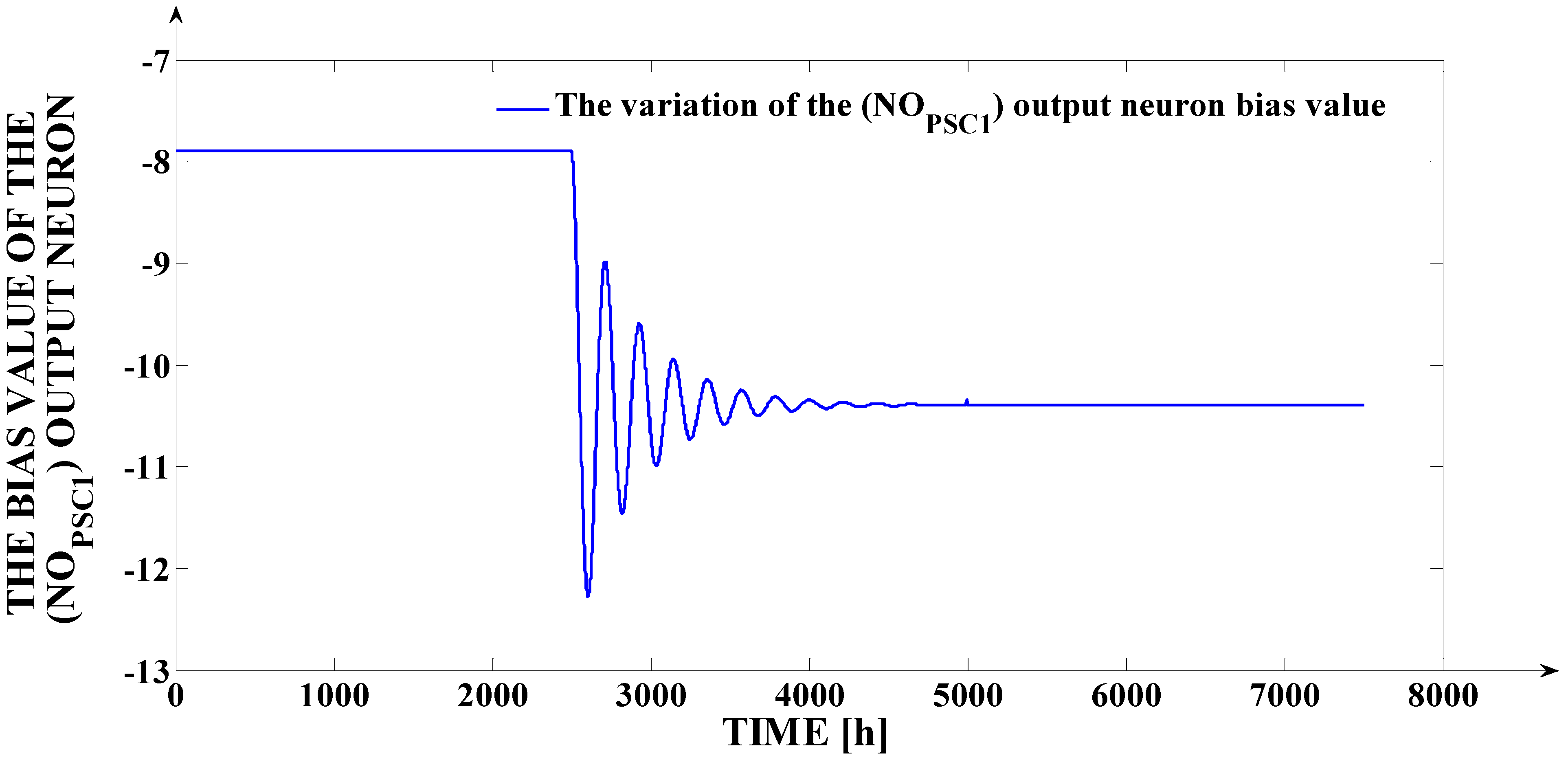
The variation, in relation to time, of the (
bOLPSC1) bias value is presented in
Figure 12. The adaptation effort is visible after the moment
t = 2500 h. Further, after the moment
t = 5000 h, the (
bOLPSC1) bias value remains constant because the
18O isotope concentration at the output of FSC is due to the (
Ff) input signal variation and not due to a parametric disturbance.
- (b)
The idea of the adaptive strategy generalization.
In near future, the problem of the proposed adaptive strategy generalization will be approached. The generalized adaptive strategy will contain in the structure the following elements:
A Decision Element, which will have the purpose of identifying the structure parameters that present variations in relation to time; in the presented example, only the variation of the SPST(Fi) function was considered as a consequence of the variation of one or more HETP1(Fi) function parameters, but during the real operation of the plant, other structure parameters can present variations, too (for example, the separation process time constants T1(Fi) and T2(Ff) or “length constants” R1(Fi) and R2(Ff)); these variations of the different separation process structure parameters can also occur, simultaneously; consequently, the identification of the process structure parameters that are affected by the parametric disturbances become necessary in order to determine which weights or bias values of the two used neural networks have to be modified as result of the adaptation effect;
The Adaptive Mechanism, which will have the same main purpose as in
Figure 9, but which will run more complex optimization algorithms (the Adaptive Mechanism will have to generate more than one adaptation signals); the Adaptive Mechanism can be implemented, also, by using AI specific methods;
A Signal Distributor which will have the purpose to distribute the adaptation signals generated by the Adaptive Mechanism to the two neural networks weights and bias values; the identification of the weights and bias values of the two neural networks, which must be modified to adapt the proposed mathematical model properly, is also made by the Adaptive Mechanism.
- (c)
The real-time identification of the separation model.
Another future possibility for obtaining the adapted mathematical model of the separation cascade is represented by the real-time learning of the process behavior. In this case, the following stages must be passed through:
The input and the output signals corresponding to the separation cascade, after their measuring and sampling, are be saved as datasets;
The resulting datasets are preprocessed;
In the case of identifying deviations of the proposed model response from the real response of the separation cascade, the two neural networks are trained again using the mentioned datasets;
The old neural solutions will be replaced with the new ones, obtained at the previous stage.
As a conclusion, the mathematical model adaptation at the occurrence of the parametric disturbances is very important due to the necessity of using it with high precision in different applications (as reference model in automatic control structure, as model for approximating the separation cascade energy consumption, as decision support for the operators, etc.)


 ,
, 


