The Distributed and Centralized Fusion Filtering Problems of Tessarine Signals from Multi-Sensor Randomly Delayed and Missing Observations under ${\mathbb{T}}_k$-Properness Conditions

Abstract

This paper addresses the fusion estimation problem in tessarine systems with multi-sensor observations affected by mixed uncertainties when under ${\mathbb{T}}_k$-properness conditions. Observations from each sensor can be updated, delayed, or contain only noise, and a correlation is assumed between the state and the observation noises. Recursive algorithms for the optimal local linear filter at each sensor as well as both centralized and distributed linear fusion estimators are derived using an innovation approach. The ${\mathbb{T}}_k$-properness assumption implies a reduction in the dimension of the augmented system, which yields computational savings in the previously mentioned algorithms compared to their counterparts, which are derived from real or widely linear processing. A numerical simulation example illustrates the obtained theoretical results and allows us to visualize, among other aspects, the insignificant difference in the accuracy of both fusion filters, which means that the distributed filter, although suboptimal, is preferable in practice as it implies a lower computational cost.

1. Introduction

In the scientific community, there has recently been increasing interest in approaching different estimation problems in systems with observations proceeding from multiple sensors. Evidently, this availability yields better estimations, since the information supplied from several sensors may compensate for the possible adverse effects of some faulty sensors, communication errors, or defects when using a single sensor. According to the way that information is fused, the estimation techniques can be categorized into two large groups: centralized and distributed methods. In the former group, all the observations from all the sensors are directly sent to the fusion center to be processed in a single fusion estimator. In the latter, the observations at each sensor are independently processed, providing a local estimator, and, afterwards, in the fusion center, a single distributed fusion estimator is built from these local estimators. Both fusion “architectures” have strengths and weaknesses, meaning that they can be used alternatively in practice, depending on the problem at hand. As is already known, the centralized method provides a theoretical, optimal solution to the estimation problem; in contrast, this may imply a heavy computational burden, and a high bandwidth may be required. Moreover, the architecture cannot be changed [1,2,3,4]. In contrast, the situation with the distributed fusion method the opposite. This method has great advantages over the centralized one due to the fact that it requires a lower computational load and communication costs, and is more robust in terms of failure and flexibility. However, the disadvantage of this method is that the optimality condition of the estimators is lost [2,5,6]. Nevertheless, this weakness is acceptable when considering the advantages that this methodology presents, accounting for the slight difference that there may be in practice between the estimators obtained by both methods.

Furthermore, in data transmission problems, random delays, packet dropouts, or missing measurements frequently occur. These problems are caused by limited communication capabilities or some failures in transmission components. In the real domain, there is a wide-ranging literature on signal linear processing under uncertain outputs based on both centralized (see, e.g., [7,8,9], among others) and distributed fusion methods (see, e.g., [10,11,12,13,14]). In all of them, different scenarios concerning the initial state-space model and the characteristics of the observations from the sensors are considered. More specifically, by considering these three mixed uncertainties, the centralized fusion linear optimal estimation problem has been solved in [8]. In multi-sensor systems with missing measurements, the centralized and distributed fusion estimators have been obtained in [9] and [11,12], respectively, by assuming different conditions for the noise variances and updating the state at each sensor. An analysis of the effects of these packet losses has been developed in [15] for the centralized Kalman filtering and [12,16] for the distributed fusion filtering problem. Moreover, the distributed fusion estimation problem has also been studied in networked systems, for a class of uncertain sensor networks with multiple delays [7,10], and assuming correlated noises [13,14]. In the above references, the situations referring to the uncertainties in the observations are usually modeled by Bernoulli random parameters with known probabilities. Indeed, this is the most common probability distribution to describe the different types of uncertainty.

In the last two decades, the interest in hypercomplex domains has considerably grown due to their adequacy in describing a high number of physical phenomena. Their usefulness lies in the fact that they operate in higher-dimensional spaces, and are thus able to explain the relationships between the dimensions. As an example, we can mention the use of hypercomplex domains in virtual reality [17,18], acoustic applications [19,20], communication [21,22], image processing [23,24], seismic phenomena [25,26], robotics [27,28], materials [29,30], avionics [31,32], etc.

At the same time, the need to address, among other aspects, the signal processing problem by using 4D hypercomplex algebras arises. To date, quaternion algebra has been the most commonly used type of algebra in signal processing, since it is a normed division algebra. Specifically, in the optimal signal estimation problem, under the so-called widely linear (WL) processing, the signal quaternion and its three involutions have to be considered. Nevertheless, the processes involved in the model can present some properties that lead to a reduction in the dimension of the model by considering the quaternion signal itself, called strictly linear (SL) processing, or a two-dimensional vector given by the quaternion signal and its involution over the pure unit quaternion, named semi-widely linear (SWL) processing. This reduction in the dimension of the model entails a major decrease in the computational burden. In this framework, the WL estimation problem has been studied in [17,19,31] for different real problems, and algorithms based on the Kalman filter have been proposed in the quaternion field. Moreover, in multi-sensor systems, the WL distributed fusion estimation problem has been addressed in [33,34,35,36,37]. In addition, for systems with missing observations, WL and SWL filtering, prediction and smoothing algorithms have been designed in [38] and [39], respectively, with correlation hypotheses on the state and observation noises considered in the latter. Additionally, the WL estimation problem in multi-sensor systems with random delays, packet dropouts, and uncertain observations has been studied in [40]. It should be highlighted that quaternion processing is not always the most appropriate methodology. In fact, the use of tessarine signals can bring, under certain conditions, a better performance of the estimators, as has been tested in [41,42,43].

However, the signal estimation problem in the tessarine domain has hardly been studied at all. This is due to the fact that the set of tessarine random variables does not have a Hilbert space structure; therefore, it is difficult to calculate the LS linear estimator. Recently, in [41], a metric has been defined in the tessarine domain that satisfies the properties necessary to guarantee the existence and uniqueness of the projection. Moreover, by making an analogy with the quaternion domain, the authors define ${\mathbb{T}}_1$-properness, and prove that the tessarine widely linear (TWL) estimation error coincides with that of ${\mathbb{T}}_1$, which yields a considerable reduction in the computational cost of obtaining the optimal solution. Later, the ${\mathbb{T}}_2$-properness definition is established in [42], obtaining the same result for the TWL and ${\mathbb{T}}_2$ estimation errors. These types of ${\mathbb{T}}_k$-properness have been used in [43] to approach the LS linear centralized fusion estimation problem of signals from multi-sensor observations with random delays.

Considering these benefits for the ${\mathbb{T}}_k$-properness, in this paper, we address both distributed and centralized fusion LS estimation problems in tessarine systems with mixed uncertainties of randomly delayed and missing observations proceeding from multiple sensors. At each sensor and instant of time, each tessarine component can be updated, delayed, or contain only noise, independently of the remaining sensors. We have also assumed a correlation between the signal and observation noises, which is a very desirable property for multi-sensor systems, since the observations act as output feedback [14]. By using an innovation approach, recursive algorithms are derived to compute the LS distributed and centralized fusion filters. These have been characterized for both ${\mathbb{T}}_k$-proper scenarios, where the reduction in the system dimension is clearly reflected. A decrease in the computational burden can also be observed by using the distributed filtering algorithm instead of the centralized one and, although the distributed algorithm provides suboptimal estimators, a simulation example shows that the differences between them may be insignificant in practice.

The rest of the paper is organized as follows. In Section 2, the notation that will be used throughout the paper is established, as well as a revision of the main concepts and results in the tessarine domain. Next, in Section 3, the tessarine state and observation equations (both the real and available ones) are established, as well as the hypotheses on the processes involved. The different mixed uncertainties are modelled by using Bernoulli random variables with known parameters, whose values of one or zero determine if an observation is updated, delayed, or contains only noise. Then, the augmented model (by considering the three conjugations) is presented in Section 4, and the conditions for the processes which guarantee ${\mathbb{T}}_k$-properness are studied. The reduction in the model under these ${\mathbb{T}}_k$-properness conditions is shown and, in this scenario, a recursive algorithm is proposed to obtain the local optimal LS linear filtering estimators. Subsequently, in Section 5, by considering the compact model, that is, the observations from all the sensors, a recursive algorithm is devised to obtain the optimal LS linear centralized fusion filter under ${\mathbb{T}}_k$-properness conditions. Adittionally, a method for the recursive computation of the ${\mathbb{T}}_k$ distributed fusion filter as the LS matrix-weighted linear combination of the optimal local LS linear estimators is proposed in Section 6. Afterwards, a numerical simulation example in Section 7 illustrates several items: (i) the superiority of both fusion filters over the local ones, (ii) the performance of the fusion filters increases as the updating and delay probabilities become greater and by comparing the same probability that the observation is updated or delayed; (iii) the accuracy of the centralized fusion filter is better than the distributed one, but the difference is almost insignificant. Finally, a section of conclusions (Section 8) and two appendixes with the proofs of all the results in the paper have been included.

2. Preliminaries

In this section, we introduce the basic notation that will be used in this paper. Matrices will be written in bold, upper-case letters, column vectors in bold, lower-case letters, and scalar quantities in lightfaced letters. We will use the superscripts “*”, “$\mathtt{T}$” and “$\mathtt{H}$” to represent the tessarine conjugate, transpose and conjugate transpose, respectively. For ${\mathbf{0}}_{n\times m}$, we will denote the $n\times m$ zero matrix, ${\mathbf{I}}_n$ the identity matrix of dimension n, and ${\mathbf{1}}_n$ and ${\mathbf{0}}_n$, the column vector of dimension n with all its elements 1 or 0, respectively. Letters $\mathbb{Z}$, $\mathbb{R}$ and $\mathbb{T}$ will represent the set of integer, real and tessarine field, respectively. Moreover, $\mathbf{A}\in {\mathbb{R}}^{n\times m}$ (respectively, $\mathbf{A}\in {\mathbb{T}}^{n\times m}$) means that $\mathbf{A}$ is a real (respectively, tessarine) $n\times m$ matrix. Similarly, $\mathbf{r}\in {\mathbb{R}}^m$ (respectively, $\mathbf{r}\in {\mathbb{T}}^m$) means that $\mathbf{r}$ is a m-dimensional real (respectively, tessarine) vector.

In addition, $E[·]$ and $\mathrm{Cov}(·)$ will denote the expectation and covariance operators and $\mathrm{diag}(·)$ is a diagonal matrix with the elements specified on the main diagonal. Finally, “∘” and “⊗” denote the Hadamard and Kronecker products, respectively, and ${\delta }_{ts}$, the Kronecker delta function. We will use the following property of the Hadamard product:

Property 1.

If $\mathbf{A}\in {\mathbb{R}}^{n\times n}$ and $\mathbf{b}\in {\mathbb{R}}^n$, then $diag\left(\mathbf{b}\right)\mathbf{A}diag\left(\mathbf{b}\right)=\left(\mathbf{b}{\mathbf{b}}^{\mathtt{T}}\right)\circ \mathbf{A}$.

Throughout this paper, and unless otherwise stated, all the random variables are assumed to have zero-mean. Next, we present a review of the tessarine domain.

Definition 1.

A tessarine random signal $\mathbf{x}\left(t\right)\in {\mathbb{T}}^n$ is a stochastic process of the form [41]

$$\mathbf{x}\left(t\right)={\mathbf{x}}_r\left(t\right)+\eta {\mathbf{x}}_{\eta }\left(t\right)+{\eta }^{\prime }{\mathbf{x}}_{{\eta }^{\prime }}\left(t\right)+{\eta }^{″}{\mathbf{x}}_{{\eta }^{″}}\left(t\right),$$

(1)

where ${\mathbf{x}}_{\nu }\left(t\right)\in {\mathbb{R}}^n$, for $\nu =r,\eta ,{\eta }^{\prime },{\eta }^{″}$, are real random signals and the imaginary units $\{\eta ,{\eta }^{\prime },{\eta }^{″}\}$ satisfy the identities:

$$\eta {\eta }^{\prime }={\eta }^{″},{\eta }^{\prime }{\eta }^{″}=\eta ,{\eta }^{″}\eta =-{\eta }^{\prime },{\eta }^2={\eta }^{″}{}^2=-1,{\eta }^{\prime }{}^2=1.$$

These properties of the imaginary units guarantee the commutative property of the product, implying a great advantage over the quaternion algebra, in which that property is not met. In contrast, the involutions defined in the quaternion domain cannot be defined in the tessarine one because they are auto-involutive. The conjugate of the tessarine signal given in (1) is defined as

$$\mathbf{x}*\left(t\right)={\mathbf{x}}_r\left(t\right)-\eta {\mathbf{x}}_{\eta }\left(t\right)+{\eta }^{\prime }{\mathbf{x}}_{{\eta }^{\prime }}\left(t\right)-{\eta }^{″}{\mathbf{x}}_{{\eta }^{″}}\left(t\right),$$

and the auxiliary tessarines as

$$\begin{array}{c}{\mathbf{x}}^{\eta }\left(t\right)={\mathbf{x}}_r\left(t\right)+\eta {\mathbf{x}}_{\eta }\left(t\right)-{\eta }^{\prime }{\mathbf{x}}_{{\eta }^{\prime }}\left(t\right)-{\eta }^{″}{\mathbf{x}}_{{\eta }^{″}}\left(t\right),\hfill \\ {\mathbf{x}}^{{\eta }^{″}}\left(t\right)={\mathbf{x}}_r\left(t\right)-\eta {\mathbf{x}}_{\eta }\left(t\right)-{\eta }^{\prime }{\mathbf{x}}_{{\eta }^{\prime }}\left(t\right)+{\eta }^{″}{\mathbf{x}}_{{\eta }^{″}}\left(t\right).\hfill \end{array}$$

It is also defined the real vector formed with the components of $\mathbf{x}\left(t\right)$ in (1), ${\mathbf{x}}^r\left(t\right)={\left[{\mathbf{x}}_r^{\mathtt{T}}\left(t\right),{\mathbf{x}}_{\eta }^{\mathtt{T}}\left(t\right),{\mathbf{x}}_{{\eta }^{\prime }}^{\mathtt{T}}\left(t\right),{\mathbf{x}}_{{\eta }^{″}}^{\mathtt{T}}\left(t\right)\right]}^{\mathtt{T}}$, and the augmented tessarine signal vector constituted by the tessarine signal $\mathbf{x}\left(t\right)$ and its conjugations, i.e., $\overline{\mathbf{x}}\left(t\right)={\left[{\mathbf{x}}^{{}^{\mathtt{T}}}\left(t\right),{\mathbf{x}}^{*\mathtt{T}}\left(t\right),{\mathbf{x}}^{{\eta }^{\mathtt{T}}}\left(t\right),{\mathbf{x}}^{{{\eta }^{″}}^{\mathtt{T}}}\left(t\right)\right]}^{\mathtt{T}}$. The relationship between both vectors is given by the following expression

$$\overline{\mathbf{x}}\left(t\right)=2{\mathcal{T}}_n{\mathbf{x}}^r\left(t\right),$$

where ${\mathcal{T}}_n=\frac{1}{2}\mathcal{A}\otimes {\mathbf{I}}_n$, with

$$\mathcal{A}=\left[\begin{array}{cccc}\hfill 1& \hfill \eta & \hfill {\eta }^{\prime }& \hfill {\eta }^{″}\\ \hfill 1& \hfill -\eta & \hfill {\eta }^{\prime }& \hfill -{\eta }^{″}\\ \hfill 1& \hfill \eta & \hfill -{\eta }^{\prime }& \hfill -{\eta }^{″}\\ \hfill 1& \hfill -\eta & \hfill -{\eta }^{\prime }& \hfill {\eta }^{″}\end{array}\right].$$

This property is satisfied: ${\mathcal{T}}_n^{\mathtt{H}}{\mathcal{T}}_n={\mathbf{I}}_{4n}$.

As in the quaternion field ([38]), we define the following product between tessarines, which will be crucial to model the intermittency and delay in the observations.

Definition 2.

The product ★ between two tessarine signals $\mathbf{x}\left(t\right),\mathbf{y}\left(s\right)\in {\mathbb{T}}^n$ is defined as

$$\mathbf{x}\left(t\right)★\mathbf{y}\left(s\right)={\mathbf{x}}_r\left(t\right)\circ {\mathbf{y}}_r\left(s\right)+\eta {\mathbf{x}}_{\eta }\left(t\right)\circ {\mathbf{y}}_{\eta }\left(s\right)+{\eta }^{\prime }{\mathbf{x}}_{{\eta }^{\prime }}\left(t\right)\circ {\mathbf{y}}_{{\eta }^{\prime }}\left(s\right)+{\eta }^{″}{\mathbf{x}}_{{\eta }^{″}}\left(t\right)\circ {\mathbf{y}}_{{\eta }^{″}}\left(s\right).$$

The following property of the product ★ is easy to check.

Property 2.

The augmented vector of $\mathbf{x}\left(t\right)★\mathbf{y}\left(s\right)$ is $\overline{\mathbf{x}\left(t\right)★\mathbf{y}\left(s\right)}={\mathcal{D}}^{\mathbf{x}}\left(t\right)\overline{\mathbf{y}}\left(s\right)$, where ${\mathcal{D}}^{\mathbf{x}}\left(t\right)={\mathcal{T}}_n$ $diag\left({\mathbf{x}}^r\left(t\right)\right){\mathcal{T}}_n^{\mathtt{H}}$.

Definition 3.

The pseudo autocorrelation function of the random signal $\mathbf{x}\left(t\right)\in {\mathbb{T}}^n$ is defined as ${\mathsf{\Gamma }}_{\mathbf{x}}(t,s)=E\left[\mathbf{x}\left(t\right){\mathbf{x}}^{\mathtt{H}}\left(s\right)\right]$, $\forall t,s\in \mathbb{Z}$, and the pseudo cross-correlation function of the random signals $\mathbf{x}\left(t\right)\in {\mathbb{T}}^n$ and $\mathbf{y}\left(t\right)\in {\mathbb{T}}^m$ is defined as ${\mathsf{\Gamma }}_{\mathbf{x}\mathbf{y}}(t,s)=E\left[\mathbf{x}\left(t\right){\mathbf{y}}^{\mathtt{H}}\left(s\right)\right]$, $\forall t,s\in \mathbb{Z}$.

The concept of ${\mathbb{T}}_1$ and ${\mathbb{T}}_2$-properness we next define, was recently introduced in [41] and [42], respectively, and consists of the vanishing of some of the pseudo correlation functions of the signal with its conjugations, in an analogous manner to what was in the quaternion domain.

Definition 4.

A random signal $\mathbf{x}\left(t\right)\in {\mathbb{T}}^n$ is said to be ${\mathbb{T}}_1$-proper (respectively, ${\mathbb{T}}_2$-proper) if, and only if, the functions ${\mathsf{\Gamma }}_{{\mathbf{xx}}^{\nu }}(t,s)$, with $\nu =\ast ,\eta ,{\eta }^{″}$ (respectively, $\nu =\eta ,{\eta }^{″}$), vanish for all $t,s\in \mathbb{Z}$. Similarly, two random signals $\mathbf{x}\left(t\right)\in {\mathbb{T}}^n$ and $\mathbf{y}\left(t\right)\in {\mathbb{T}}^m$ are cross ${\mathbb{T}}_1$-proper (respectively, cross ${\mathbb{T}}_2$-proper) if, and only if, the functions ${\mathsf{\Gamma }}_{{\mathbf{xy}}^{\nu }}(t,s)$, with $\nu =\ast ,\eta ,{\eta }^{″}$ (respectively, $\nu =\eta ,{\eta }^{″}$), vanish for all $t,s\in \mathbb{Z}$. Finally, $\mathbf{x}\left(t\right)$ and $\mathbf{y}\left(t\right)$ are jointly ${\mathbb{T}}_1$-proper (respectively, jointly ${\mathbb{T}}_2$-proper) if, and only if, they are ${\mathbb{T}}_1$-proper (respectively, ${\mathbb{T}}_2$-proper) and cross ${\mathbb{T}}_1$-proper (respectively, cross ${\mathbb{T}}_2$-proper).

Note that, in TWL processing, the fact that ${\mathbb{T}}_k$-properness is satisfied, causes a considerable reduction in the dimensions of the processes involved, with the consequent decrease in the computational cost. More specifically, in the most general case, TWL processing uses the augmented vectors formed by the process and its three conjugations. However, if tessarine linear processing is applied by considering only the process or the process and its conjugate, then they are denominated ${\mathbb{T}}_1$ and ${\mathbb{T}}_2$ linear processing, respectively. In [41], the authors prove that, in general, the TWL estimation error is lower than that of ${\mathbb{T}}_1$, but under ${\mathbb{T}}_1$-properness conditions, both the TWL and ${\mathbb{T}}_1$ estimators coincide. Analogous considerations about ${\mathbb{T}}_2$ processing are shown in [42]. Moreover, both papers propose statistical tests to experimentally check if a signal is ${\mathbb{T}}_k$-proper, for $k=1,2$, and prove that, under certain conditions, the tessarine processing can obtain better estimators than the quaternion one. The statements above justify that the ${\mathbb{T}}_k$-properness conditions are very desirable in practice. In this sense, it will be of great interest to determine under what conditions ${\mathbb{T}}_k$-properness is guaranteed.

3. Model Formulation

Consider a tessarine state $\mathbf{x}\left(t\right)\in {\mathbb{T}}^n$ satisfying the following state equation:

$$\mathbf{x}(t+1)={\mathbf{F}}_1\left(t\right)\mathbf{x}\left(t\right)+{\mathbf{F}}_2\left(t\right)\mathbf{x}*\left(t\right)+{\mathbf{F}}_3\left(t\right){\mathbf{x}}^{\eta }\left(t\right)+{\mathbf{F}}_4\left(t\right){\mathbf{x}}^{{\eta }^{″}}\left(t\right)+\mathbf{u}\left(t\right),t\ge 0,$$

(2)

where ${\mathbf{F}}_i\left(t\right)\in {\mathbb{T}}^{n\times n}$, for $i=1,\dots ,4$, are deterministic matrices and $\mathbf{u}\left(t\right)\in {\mathbb{T}}^n$ is a tessarine noise.

We also assume that R sensors exist, providing each of them with a real observation, ${\mathbf{z}}^{\left(i\right)}\left(t\right)\in {\mathbb{T}}^n$, satisfying the following equation:

$${\mathbf{z}}^{\left(i\right)}\left(t\right)=\mathbf{x}\left(t\right)+{\mathbf{v}}^{\left(i\right)}\left(t\right),t\ge 1,i=1,\dots ,R,$$

(3)

with ${\mathbf{v}}^{\left(i\right)}\left(t\right)\in {\mathbf{T}}^n$ a tessarine noise.

As it occurs in multiple practical situations, due to failures in communication channels, network congestion or some other causes, the available observations can suffer delays and even contain only noise in an intermittent manner. This fact can be modelled by the following equation for the available observation in each sensor, ${\mathbf{y}}^{\left(i\right)}\left(t\right)\in {\mathbb{T}}^n$, for $i=1,\dots ,R$:

$$\begin{array}{cc}\hfill {\mathbf{y}}^{\left(i\right)}\left(t\right)& ={\gamma }_1^{\left(i\right)}\left(t\right)☆{\mathbf{z}}^{\left(i\right)}\left(t\right)+{\gamma }_2^{\left(i\right)}\left(t\right)☆{\mathbf{z}}^{\left(i\right)}(t-1)\hfill \\ \hfill & +({\mathbf{1}}_n-{\gamma }_1^{\left(i\right)}\left(t\right)-{\gamma }_2^{\left(i\right)}\left(t\right))☆{\mathbf{v}}^{\left(i\right)}\left(t\right),t\ge 2;\hfill \\ \hfill {\mathbf{y}}^{\left(i\right)}\left(1\right)& ={\mathbf{z}}^{\left(i\right)}\left(1\right).\hfill \end{array}$$

(4)

For each sensor $i=1,\dots ,R$ and for $j=1,2$, ${\gamma }_j^{\left(i\right)}\left(t\right)={[{\gamma }_{j_1}^{\left(i\right)}\left(t\right),\dots ,{\gamma }_{j_n}^{\left(i\right)}\left(t\right)]}^T\in {\mathbb{T}}^n$ is a tessarine random vector whose components are composed by independent Bernoulli random variables ${\gamma }_{j_m,\nu }^{\left(i\right)}\left(t\right)$, with $m=1,\dots ,n,\nu =r,\eta ,{\eta }^{\prime },{\eta }^{″}$ with known probabilities $p_{j_m,\nu }^{\left(i\right)}\left(t\right)$, respectively. Values of one or zero for these Bernoulli variables indicate if the corresponding component of the available observation is updated, one-step delayed or only contains noise. These variables must satisfy that, for each $i=1,\dots ,R,m=1,\dots ,n,\nu =r,\eta ,{\eta }^{\prime },{\eta }^{″}$, ${\gamma }_{1_m,\nu }^{\left(i\right)}\left(t\right)+{\gamma }_{2_m,\nu }^{\left(i\right)}\left(t\right)=1$ or ${\gamma }_{1_m,\nu }^{\left(i\right)}\left(t\right)+{\gamma }_{2_m,\nu }^{\left(i\right)}\left(t\right)=0$ at each instant of time; that is, if one of them takes value 1, the other one is 0, or both are 0; moreover, $p_{1_m,\nu }^{\left(i\right)}\left(t\right)+p_{2_m,\nu }^{\left(i\right)}\left(t\right)\le 1$. In this sense, if ${\gamma }_{1_m,\nu }^{\left(i\right)}\left(t\right)=1$, then $y_{m,\nu }^{\left(i\right)}\left(t\right)=z_{m,\nu }^{\left(i\right)}\left(t\right)$; that is, it contains the updated observation component; if ${\gamma }_{2_m,\nu }^{\left(i\right)}\left(t\right)=1$, then $y_{m,\nu }^{\left(i\right)}\left(t\right)=z_{m,\nu }^{\left(i\right)}(t-1)$, the available observation component is that delayed one instant of time and, finally, if ${\gamma }_{1_m,\nu }^{\left(i\right)}\left(t\right)={\gamma }_{2_m,\nu }^{\left(i\right)}\left(t\right)=0$, then $y_{m,\nu }^{\left(i\right)}\left(t\right)=v_{m,\nu }^{\left(i\right)}\left(t\right)$; that is, it contains only noise. Observe that the initial available observation is updated.

We assume the following hypotheses for the model defined in (2)–(4):

Hypothesis 1 (H1).

$\left\{\mathbf{u}\right(t);t\ge 0\}$ and $\{{\mathbf{v}}^{\left(i\right)}\left(t\right);t\ge 1\}$, $i=1,\dots ,R$ are white noises with pseudo variances $\mathbf{Q}\left(t\right)$ and ${\mathbf{R}}^{\left(i\right)}\left(t\right)$, respectively. Moreover, they are correlated at the same instant of time, with $E\left[\mathbf{u}\left(t\right){\mathbf{v}}^{{\left(i\right)}^{\mathtt{H}}}\left(t\right)\right]={\mathbf{S}}^{\left(i\right)}\left(t\right)$.

Hypothesis 2 (H2).

${\mathbf{v}}^{\left(i\right)}\left(t\right)$ is independent of ${\mathbf{v}}^{\left(j\right)}\left(t\right)$ for $i,j=1,\dots ,R$, with $i\ne j$.

Hypothesis 3 (H3).

For each sensor $i=1,\dots R$, and $j=1,2$, the Bernoulli variables in ${\gamma }_j^{\left(i\right)}\left(t\right)$ are independent of those in ${\gamma }_j^{\left(i\right)}\left(s\right)$, for $s\ne t$. The same hypothesis for ${\gamma }_j^{\left(i\right)}\left(t\right)$ and ${\gamma }_j^{\left(l\right)}\left(t\right)$ with $i\ne l$.

Hypothesis 4 (H4).

The initial state, $\mathbf{x}\left(0\right)$, (whose pseudo variance is denoted by ${\mathbf{P}}_0$) and the noises $\left\{\mathbf{u}\right(t);t\ge 0\}$, $\{{\mathbf{v}}^{\left(i\right)}\left(t\right);t\ge 1\}$ and $\{{\gamma }_j^{\left(i\right)}\left(t\right);t\ge 2\}$, for $j=1,2$, $i=1,\dots ,R$, are mutually independent.

An example of the above scenario can be found in the problem of dynamic targeting tracking (see, e.g., [13]) and, in particular, in the problem of tracking the rotations of an aircraft [35,36].

4. Local ${\mathbb{T}}_{\mathbf{k}}$-Proper LS Linear Filtering Problem

In this section, the local LS linear filtering problem is studied for the tessarine model described above; that is, for each sensor $i=1,\dots ,R$, the optimal lineal estimation problem of the signal $\mathbf{x}\left(t\right)$ is addressed from the observations provided by that sensor i. For this purpose, firstly, the model is formulated at each sensor, by considering both delays and the internittency in the avilable observation equation. Moreover, due to the great computational advantages, the conditions on the processes involved to ensure ${\mathbb{T}}_k$-properness are proposed. Once the model has been formulated, a recursive algorithm is presented to obtain the optimal local LS linear filters. In Section 6, this algorithm will be necessary to address the distributed fusion LS linear filtering problem.

4.1. Local ${\mathbb{T}}_k$-Proper Model Formulation

For each sensor $i=1,\dots ,R$, the augmented version of the model defined in Equations (2)–(4) is as follows

$$\begin{array}{cc}\hfill \overline{\mathbf{x}}(t+1)& =\overline{\mathsf{\Phi }}\left(t\right)\overline{\mathbf{x}}\left(t\right)+\overline{\mathbf{u}}\left(t\right),t\ge 0,\hfill \\ \hfill {\overline{\mathbf{z}}}^{\left(i\right)}\left(t\right)& =\overline{\mathbf{x}}\left(t\right)+{\overline{\mathbf{v}}}^{\left(i\right)}\left(t\right),t\ge 1,\hfill \\ \hfill {\overline{\mathbf{y}}}^{\left(i\right)}\left(t\right)& ={\mathcal{D}}^{{\gamma }_1^{\left(i\right)}}\left(t\right){\overline{\mathbf{z}}}^{\left(i\right)}\left(t\right)+{\mathcal{D}}^{{\gamma }_2^{\left(i\right)}}\left(t\right){\overline{\mathbf{z}}}^{\left(i\right)}(t-1)\hfill \\ \hfill & +{\mathcal{D}}^{\mathbf{1}-{\gamma }_1^{\left(i\right)}-{\gamma }_2^{\left(i\right)}}\left(t\right){\overline{\mathbf{v}}}^{\left(i\right)}\left(t\right),t\ge 2;{\overline{\mathbf{y}}}^{\left(i\right)}\left(1\right)={\overline{\mathbf{z}}}^{\left(i\right)}\left(1\right),\hfill \end{array}$$

(5)

where

$$\overline{\mathsf{\Phi }}\left(t\right)=\left[\begin{array}{cccc}{\mathbf{F}}_1\left(t\right)& {\mathbf{F}}_2\left(t\right)& {\mathbf{F}}_3\left(t\right)& {\mathbf{F}}_4\left(t\right)\\ {\mathbf{F}}_2^{\ast }\left(t\right)& {\mathbf{F}}_1^{\ast }\left(t\right)& {\mathbf{F}}_4^{\ast }\left(t\right)& {\mathbf{F}}_3^{\ast }\left(t\right)\\ {\mathbf{F}}_3^{\eta }\left(t\right)& {\mathbf{F}}_4^{\eta }\left(t\right)& {\mathbf{F}}_1^{\eta }\left(t\right)& {\mathbf{F}}_2^{\eta }\left(t\right)\\ {\mathbf{F}}_4^{{\eta }^{″}}\left(t\right)& {\mathbf{F}}_3^{{\eta }^{″}}\left(t\right)& {\mathbf{F}}_2^{{\eta }^{″}}\left(t\right)& {\mathbf{F}}_1^{{\eta }^{″}}\left(t\right)\end{array}\right],$$

with ${\mathcal{D}}^{{\gamma }_j^{\left(i\right)}}\left(t\right)$, for $j=1,2$, and ${\mathcal{D}}^{\mathbf{1}-{\gamma }_1^{\left(i\right)}-{\gamma }_2^{\left(i\right)}}\left(t\right)$, defined in Property 2. Moreover, the pseudo variances of the augmented white noises $\overline{\mathbf{u}}\left(t\right)$ and ${\overline{\mathbf{v}}}^{\left(i\right)}\left(t\right)$ are denoted by $\overline{\mathbf{Q}}\left(t\right)$ and ${\overline{\mathbf{R}}}^{\left(i\right)}\left(t\right)$, respectively, $E\left[\overline{\mathbf{u}}\left(t\right){\overline{\mathbf{v}}}^{{\left(i\right)}^{\mathtt{H}}}\left(s\right)\right]={\overline{\mathbf{S}}}^{\left(i\right)}\left(t\right){\delta }_{t,s}$, and $E\left[\overline{\mathbf{x}}\left(0\right){\overline{\mathbf{x}}}^{\mathtt{H}}\left(0\right)\right]={\overline{\mathbf{P}}}_0$.

Next, conditions for the processes involved in (5), which guarantee a ${\mathbb{T}}_k$-properness scenario, are given in Property 3.

Property 3.

Consider the model described in Equation (5):

1.

If $\mathbf{x}\left(0\right)$ and $\mathbf{u}\left(t\right)$ are ${\mathbb{T}}_1$-proper, and $\overline{\mathsf{\Phi }}\left(t\right)$ is a block diagonal matrix of the form

$$\overline{\mathsf{\Phi }}\left(t\right)=diag\left({\mathbf{F}}_1\left(t\right),{\mathbf{F}}_1^{\ast }\left(t\right),{\mathbf{F}}_1^{\eta }\left(t\right),{\mathbf{F}}_1^{{\eta }^{″}}\left(t\right)\right),$$

then $\mathbf{x}\left(t\right)$ is ${\mathbb{T}}_1$-proper. If additionally $p_{jm,r}^{\left(i\right)}\left(t\right)=p_{jm,\eta }^{\left(i\right)}\left(t\right)=p_{jm,{\eta }^{\prime }}^{\left(i\right)}\left(t\right)=p_{jm,{\eta }^{″}}^{\left(i\right)}\left(t\right)\equiv p_{jm}^{\left(i\right)}\left(t\right)$, $\forall t,j,m,i$, ${\mathbf{v}}^{\left(i\right)}\left(t\right)$ is ${\mathbb{T}}_1$-proper, and $\mathbf{u}\left(t\right)$ and ${\mathbf{v}}^{\left(i\right)}\left(t\right)$ are cross ${\mathbb{T}}_1$-proper, then $\mathbf{x}\left(t\right)$ and ${\mathbf{y}}^{\left(i\right)}\left(t\right)$ are jointly ${\mathbb{T}}_1$-proper. In this scenario,

$${\mathbf{\Pi }}^{{\gamma }_j^{\left(i\right)}}\left(t\right)=E\left[{\mathcal{D}}^{{\gamma }_j^{\left(i\right)}}\left(t\right)\right]={\mathbf{I}}_4\otimes {\mathbf{\Pi }}_1^{j^{\left(i\right)}}\left(t\right),i=1,\dots ,R,j=1,2,$$

with

$${\mathbf{\Pi }}_1^{j^{\left(i\right)}}\left(t\right)=diag\left(p_{j1,r}^{\left(i\right)}\left(t\right),\dots ,p_{jn,r}^{\left(i\right)}\left(t\right)\right),i=1,\dots ,R,j=1,2.$$

Moreover, ${\mathbf{\Pi }}^{\mathbf{1}-{\gamma }_1^{\left(i\right)}-{\gamma }_2^{\left(i\right)}}\left(t\right)=E\left[{\mathcal{D}}^{\mathbf{1}-{\gamma }_1^{\left(i\right)}-{\gamma }_2^{\left(i\right)}}\left(t\right)\right]={\mathbf{I}}_{4n}-{\mathbf{\Pi }}^{{\gamma }_1^{\left(i\right)}}\left(t\right)-{\mathbf{\Pi }}^{{\gamma }_2^{\left(i\right)}}\left(t\right)$.

2.

By substituting in the last item ${\mathbb{T}}_1$ by ${\mathbb{T}}_2$ and the matrix $\overline{\mathsf{\Phi }}\left(t\right)$ by this other

$$\overline{\mathsf{\Phi }}\left(t\right)=diag\left({\mathsf{\Phi }}_2\left(t\right),{\mathsf{\Phi }}_2^{\eta }\left(t\right)\right),\mathrm{with}{\mathsf{\Phi }}_2\left(t\right)=\left[\begin{array}{cc}{\mathbf{F}}_1\left(t\right)& {\mathbf{F}}_2\left(t\right)\\ {\mathbf{F}}_2^{\ast }\left(t\right)& {\mathbf{F}}_1^{\ast }\left(t\right)\end{array}\right],$$

(6)

and assuming that the Bernoulli parameters now satisfy that $p_{jm,r}^{\left(i\right)}\left(t\right)=p_{jm,\eta }^{\left(i\right)}\left(t\right)$ and $p_{jm,{\eta }^{\prime }}^{\left(i\right)}\left(t\right)=p_{jm,{\eta }^{″}}^{\left(i\right)}\left(t\right)$, $\forall t,j,m,i$, an identical property can be established for the joint ${\mathbb{T}}_2$-properness of $\mathbf{x}\left(t\right)$ and ${\mathbf{y}}^{\left(i\right)}\left(t\right)$. In this case, the expectation of the multiplicative noises are given by

$$\begin{array}{cc}\hfill {\mathbf{\Pi }}^{{\gamma }_j^{\left(i\right)}}\left(t\right)& =diag\left({\mathbf{\Pi }}_2^{j^{\left(i\right)}}\left(t\right),{\mathbf{\Pi }}_2^{j^{\left(i\right)}}\left(t\right)\right),i=1,\dots ,R,j=1,2,\hfill \\ \hfill {\mathbf{\Pi }}^{\mathbf{1}-{\gamma }_1^{\left(i\right)}-{\gamma }_2^{\left(i\right)}}\left(t\right)& ={\mathbf{I}}_{4n}-{\mathbf{\Pi }}^{{\gamma }_1^{\left(i\right)}}\left(t\right)-{\mathbf{\Pi }}^{{\gamma }_2^{\left(i\right)}}\left(t\right),i=1,\dots ,R,\hfill \end{array}$$

with

$$\begin{array}{c}{\mathbf{\Pi }}_2^{j^{\left(i\right)}}\left(t\right)={\displaystyle \frac{1}{2}}\left[\begin{array}{cc}{\mathbf{\Pi }}_a^{j^{\left(i\right)}}\left(t\right)& {\mathbf{\Pi }}_b^{j^{\left(i\right)}}\left(t\right)\\ {\mathbf{\Pi }}_b^{j^{\left(i\right)}}\left(t\right)& {\mathbf{\Pi }}_a^{j^{\left(i\right)}}\left(t\right)\end{array}\right],i=1,\dots ,R,j=1,2,\end{array}$$

and

$$\begin{array}{c}{\mathbf{\Pi }}_a^{j^{\left(i\right)}}\left(t\right)=diag\left(p_{j1,r}^{\left(i\right)}\left(t\right)+p_{j1,{\eta }^{\prime }}^{\left(i\right)}\left(t\right),\dots ,p_{jn,r}^{\left(i\right)}\left(t\right)+p_{jn,{\eta }^{\prime }}^{\left(i\right)}\left(t\right)\right),i=1,\dots ,R,j=1,2,\\ {\mathbf{\Pi }}_b^{j^{\left(i\right)}}\left(t\right)=diag\left(p_{j1,r}^{\left(i\right)}\left(t\right)-p_{j1,{\eta }^{\prime }}^{\left(i\right)}\left(t\right),\dots ,p_{jn,r}^{\left(i\right)}\left(t\right)-p_{jn,{\eta }^{\prime }}^{\left(i\right)}\left(t\right)\right),i=1,\dots ,R,j=1,2.\end{array}$$

Note that these ${\mathbb{T}}_k$-property conditions allow us to reduce the dimension of the available observations; that is, ${\mathbf{y}}_1^{\left(i\right)}\left(t\right)\triangleq {\mathbf{y}}^{\left(i\right)}\left(t\right)$ and ${\mathbf{y}}_2^{\left(i\right)}\left(t\right)\triangleq {\left[{\mathbf{y}}^{{\left(i\right)}^T}\left(t\right),{\mathbf{y}}^{{\left(i\right)}^{\mathtt{H}}}\left(t\right)\right]}^T$, for ${\mathbb{T}}_1$ and ${\mathbb{T}}_2$-proper scenarios, respectively, and hence, the observation equation given in (5) is now expressed in the following terms:

$$\begin{array}{cc}\hfill {\mathbf{y}}_k^{\left(i\right)}\left(t\right)& ={\mathcal{D}}_k^{{\gamma }_1^{\left(i\right)}}\left(t\right){\overline{\mathbf{z}}}^{\left(i\right)}\left(t\right)+{\mathcal{D}}_k^{{\gamma }_2^{\left(i\right)}}\left(t\right){\overline{\mathbf{z}}}^{\left(i\right)}(t-1)\hfill \\ \hfill & +{\mathcal{D}}_k^{\mathbf{1}-{\gamma }_1^{\left(i\right)}-{\gamma }_2^{\left(i\right)}}\left(t\right){\overline{\mathbf{v}}}^{\left(i\right)}\left(t\right),t\ge 2;{\mathbf{y}}_k^{\left(i\right)}\left(1\right)=\left[{\mathbf{I}}_{kn},{\mathbf{0}}_{kn\times (4-k)n}\right]{\overline{\mathbf{z}}}^{\left(i\right)}\left(1\right),\hfill \end{array}$$

(7)

where

$$\begin{array}{cc}\hfill {\mathcal{D}}_k^{{\gamma }_j^{\left(i\right)}}\left(t\right)& ={\mathcal{T}}_{k}diag\left({\gamma }_j^{{\left(i\right)}^r}\left(t\right)\right){\mathcal{T}}_n^{\mathtt{H}},i=1,\dots ,R,j=1,2,\hfill \\ \hfill {\mathcal{D}}_k^{\mathbf{1}-{\gamma }_1^{\left(i\right)}-{\gamma }_2^{\left(i\right)}}\left(t\right)& ={\mathcal{T}}_{k}diag\left({\mathbf{1}}_{4n}-{\gamma }_1^{{\left(i\right)}^r}\left(t\right)-{\gamma }_2^{{\left(i\right)}^r}\left(t\right)\right){\mathcal{T}}_n^{\mathtt{H}},i=1,\dots ,R,\hfill \end{array}$$

with

$${\mathcal{T}}_k=\frac{1}{2}{\mathcal{B}}_k\otimes {\mathbf{I}}_n,$$

(8)

and

$${\mathcal{B}}_k=\left\{\begin{array}{c}\left[1\eta {\eta }^{\prime }{\eta }^{″}\right],\mathrm{for}k=1\hfill \\ \left[\begin{array}{cccc}1& \eta & {\eta }^{\prime }& {\eta }^{″}\\ 1& -\eta & {\eta }^{\prime }& -{\eta }^{″}\end{array}\right],\mathrm{for}k=2.\hfill \end{array}\right.$$

Moreover, under ${\mathbb{T}}_k$-properness, for $i=1,\dots ,R$ and $j=1,2$,

$$\begin{array}{cc}\hfill {\mathbf{\Pi }}_k^{{\gamma }_j^{\left(i\right)}}\left(t\right)=E\left[{\mathcal{D}}_k^{{\gamma }_j^{\left(i\right)}}\left(t\right)\right]& =\left[{\mathbf{\Pi }}_k^{j^{\left(i\right)}}\left(t\right),{\mathbf{0}}_{kn\times (4-k)n}\right],\hfill \\ \hfill {\mathbf{\Pi }}_k^{\mathbf{1}-{\gamma }_1^{\left(i\right)}-{\gamma }_2^{\left(i\right)}}\left(t\right)=E\left[{\mathcal{D}}_k^{\mathbf{1}-{\gamma }_1^{\left(i\right)}-{\gamma }_2^{\left(i\right)}}\left(t\right)\right]& =\left[{\mathbf{I}}_{kn}-{\mathbf{\Pi }}_k^{1^{\left(i\right)}}\left(t\right)-{\mathbf{\Pi }}_k^{2^{\left(i\right)}}\left(t\right),{\mathbf{0}}_{kn\times (4-k)n}\right],\hfill \end{array}$$

(9)

where the matrices ${\mathbf{\Pi }}_k^{j^{\left(i\right)}}\left(t\right)$, for $k=1,2$, are defined in Property 3.

Remark 1.

Let us observe that the ${\mathbb{T}}_k$-properness also causes a dimension reduction in the remaining processes and matrices involved in Equation (5). More specifically, in the ${\mathbb{T}}_1$-proper scenario, $\overline{\mathbf{x}}\left(t\right)$, $\overline{\mathbf{u}}\left(t\right)$ ${\overline{\mathbf{z}}}^{\left(i\right)}\left(t\right)$, ${\overline{\mathbf{v}}}^{\left(i\right)}\left(t\right)$ and $\overline{\mathsf{\Phi }}\left(t\right)$, are substituted by ${\mathbf{x}}_1\left(t\right)\triangleq \mathbf{x}\left(t\right)$, ${\mathbf{u}}_1\left(t\right)\triangleq \mathbf{u}\left(t\right)$, ${\mathbf{z}}_1^{\left(i\right)}\left(t\right)\triangleq {\mathbf{z}}^{\left(i\right)}\left(t\right)$, ${\mathbf{v}}_1^{\left(i\right)}\left(t\right)\triangleq {\mathbf{v}}^{\left(i\right)}\left(t\right)$ and ${\mathsf{\Phi }}_1\left(t\right)\triangleq {\mathbf{F}}_1\left(t\right)$; and, in the ${\mathbb{T}}_2$-proper scenario, by ${\mathbf{x}}_2\left(t\right)\triangleq {\left[\mathbf{x}\left(t\right),{\mathbf{x}}^{\mathtt{H}}\left(t\right)\right]}^{\mathtt{T}}$, ${\mathbf{u}}_2\left(t\right)\triangleq {\left[\mathbf{u}\left(t\right),{\mathbf{u}}^{\mathtt{H}}\left(t\right)\right]}^{\mathtt{T}}$, ${\mathbf{z}}_2^{\left(i\right)}\left(t\right)\triangleq {\left[{\mathbf{z}}^{\left(i\right)}\left(t\right),{\mathbf{z}}^{{\left(i\right)}^{\mathtt{H}}}\left(t\right)\right]}^{\mathtt{T}}$, ${\mathbf{v}}_2^{\left(i\right)}\left(t\right)\triangleq {\left[{\mathbf{v}}^{\left(i\right)}\left(t\right),{\mathbf{v}}^{{\left(i\right)}^{\mathtt{H}}}\left(t\right)\right]}^{\mathtt{T}}$ and ${\mathsf{\Phi }}_2\left(t\right)$ (given in (6)). The corresponding pseudo variance matrices of the noises ${\mathbf{u}}_k\left(t\right)$ and ${\mathbf{v}}_k^{\left(i\right)}\left(t\right)$ as well as its pseudo cross-covariance matrix, will be denoted by ${\mathbf{Q}}_k\left(t\right)$, ${\mathbf{R}}_k^{\left(i\right)}\left(t\right)$, and ${\mathbf{S}}_k^{\left(i\right)}\left(t\right)$, respectively; moreover, ${\mathbf{P}}_{0_k}=E\left[{\mathbf{x}}_k\left(0\right){\mathbf{x}}_k^{\mathtt{H}}\left(0\right)\right]$.

4.2. Local LS Filtering Estimators

Given the model described in (5), with the available observation equation in (7) for the ${\mathbb{T}}_k$-proper scenarios, a recursive algorithm to calculate the local LS filtering estimators is presented in this section. This estimator, denoted by ${\widehat{\mathbf{x}}}^{{\left(i\right)}^{{\mathbb{T}}_k}}\left(t\right|t)$, represents at each sensor i, the optimal LS linear estimator of the signal $\mathbf{x}\left(t\right)$ from the observations $\left\{{\mathbf{y}}_k^{\left(i\right)}\left(1\right),\dots ,{\mathbf{y}}_k^{\left(i\right)}\left(t\right)\right\}$. Note that this estimator can be obtained by projecting $\mathbf{x}\left(t\right)$ over the linear space spanned by the observations $\left\{{\mathbf{y}}_k^{\left(i\right)}\left(1\right),\dots ,{\mathbf{y}}_k^{\left(i\right)}\left(t\right)\right\}$. At the tessarine domain, the existence and uniqueness of this projection is guaranteed ([41]). To derive this algorithm, the innovations are used, instead of the observations, defined as ${ϵ}_k^{\left(i\right)}\left(t\right)={\mathbf{y}}_k^{\left(i\right)}\left(t\right)-{\widehat{\mathbf{y}}}_k^{\left(i\right)}\left(t\right|t-1)$, with ${\widehat{\mathbf{y}}}_k^{\left(i\right)}\left(t\right|t-1)$ the optimal LS linear estimator of the observation ${\mathbf{y}}_k^{\left(i\right)}\left(t\right)$ from the observations until the previous instant, that is, $\left\{{\mathbf{y}}_k^{\left(i\right)}\left(1\right),\dots ,{\mathbf{y}}_k^{\left(i\right)}(t-1)\right\}$.

Theorem 1.

For each sensor $i=1,\dots ,R$, the optimal filter, ${\widehat{\mathbf{x}}}^{{\left(i\right)}^{{\mathbb{T}}_k}}\left(t\right|t)$, is obtained by extracting the first n components of ${\widehat{\mathbf{x}}}_k^{\left(i\right)}\left(t\right|t)$, which satisfies this expression

$${\widehat{\mathbf{x}}}_k^{\left(i\right)}\left(t\right|t)={\widehat{\mathbf{x}}}_k^{\left(i\right)}\left(t\right|t-1)+{\mathbf{L}}_k^{\left(i\right)}\left(t\right){ϵ}_k^{\left(i\right)}\left(t\right),t\ge 1,$$

(10)

where ${\widehat{\mathbf{x}}}_k^{\left(i\right)}(t+1|t)$, can be recursively calculated as

$${\widehat{\mathbf{x}}}_k^{\left(i\right)}(t+1|t)={\mathsf{\Phi }}_k\left(t\right){\widehat{\mathbf{x}}}_k^{\left(i\right)}\left(t\right|t)+{\mathbf{H}}_k^{\left(i\right)}\left(t\right){ϵ}_k^{\left(i\right)}\left(t\right),t\ge 1,$$

(11)

with initial conditions ${\widehat{\mathbf{x}}}_k^{\left(i\right)}\left(1\right|0)={\widehat{\mathbf{x}}}_k^{\left(i\right)}\left(0\right|0)={\mathbf{0}}_{kn}$, ${\mathbf{L}}_k^{\left(i\right)}\left(t\right)={\mathsf{\Theta }}_k^{\left(i\right)}\left(t\right){\mathsf{\Omega }}_k^{{\left(i\right)}^{-1}}\left(t\right)$ and ${\mathbf{H}}_k^{\left(i\right)}\left(t\right)={\mathbf{S}}_k^{\left(i\right)}\left(t\right)\left({\mathbf{I}}_{kn}-{\mathbf{\Pi }}_k^{2^{\left(i\right)}}\left(t\right)\right){\mathsf{\Omega }}_k^{{\left(i\right)}^{-1}}\left(t\right)$.

The innovations, ${ϵ}_k^{\left(i\right)}\left(t\right)$, satisfy this relation

$$\begin{array}{cc}\hfill {ϵ}_k^{\left(i\right)}\left(t\right)& ={\mathbf{y}}_k^{\left(i\right)}\left(t\right)-{\mathbf{\Pi }}_k^{1^{\left(i\right)}}\left(t\right){\widehat{\mathbf{x}}}_k^{\left(i\right)}\left(t\right|t-1)\hfill \\ \hfill & -{\mathbf{\Pi }}_k^{2^{\left(i\right)}}\left(t\right)\left({\widehat{\mathbf{x}}}_k^{\left(i\right)}(t-1|t-1)+{\mathbf{G}}_k^{\left(i\right)}(t-1){ϵ}_k^{\left(i\right)}(t-1)\right),t\ge 2,\hfill \end{array}$$

(12)

with initial condition ${ϵ}_k^{\left(i\right)}\left(1\right)={\mathbf{y}}_k^{\left(i\right)}\left(1\right)$ and ${\mathbf{G}}_k^{\left(i\right)}\left(t\right)={\mathbf{R}}_k^{\left(i\right)}\left(t\right)\left({\mathbf{I}}_{kn}-{\mathbf{\Pi }}_k^{2^{\left(i\right)}}\left(t\right)\right){\mathsf{\Omega }}_k^{{\left(i\right)}^{-1}}\left(t\right)$.

Moreover, the matrices ${\mathsf{\Theta }}_k^{\left(i\right)}\left(t\right)$ are obtained by this expression

$$\begin{array}{cc}\hfill {\mathsf{\Theta }}_k^{\left(i\right)}\left(t\right)& ={\mathbf{P}}_k^{\left(i\right)}\left(t\right|t-1){\mathbf{\Pi }}_k^{1^{\left(i\right)}}\left(t\right)+{\mathsf{\Phi }}_k(t-1){\mathbf{P}}_k^{\left(i\right)}(t-1|t-1){\mathbf{\Pi }}_k^{2^{\left(i\right)}}\left(t\right)\hfill \\ \hfill & -{\mathbf{H}}_k^{\left(i\right)}(t-1){\left({\mathsf{\Theta }}_k^{\left(i\right)}(t-1)+{\mathbf{G}}_k^{\left(i\right)}(t-1){\mathsf{\Omega }}_k^{\left(i\right)}(t-1)\right)}^{\mathtt{H}}{\mathbf{\Pi }}_k^{2^{\left(i\right)}}\left(t\right)\hfill \\ \hfill & +\left({\mathbf{S}}_k^{\left(i\right)}(t-1)-{\mathsf{\Phi }}_k(t-1){\mathsf{\Theta }}_k^{\left(i\right)}(t-1){\mathbf{G}}_k^{{\left(i\right)}^{\mathtt{H}}}(t-1)\right){\mathbf{\Pi }}_k^{2^{\left(i\right)}}\left(t\right),t\ge 2;\hfill \\ \hfill {\mathsf{\Theta }}_k^{\left(i\right)}\left(1\right)& ={\mathbf{D}}_k\left(1\right),\hfill \end{array}$$

(13)

with

$${\mathbf{D}}_k\left(1\right)=\left[{\mathbf{I}}_{kn},{\mathbf{0}}_{kn\times (4-k)n}\right]\overline{\mathbf{D}}\left(1\right){\left[{\mathbf{I}}_{kn},{\mathbf{0}}_{kn\times (4-k)n}\right]}^{\mathtt{T}},$$

(14)

and $\overline{\mathbf{D}}\left(1\right)$ given in (16).

The pseudo-covariance matrix of the innovations, ${\mathsf{\Omega }}_k^{\left(i\right)}\left(t\right)=E\left[{ϵ}_k^{\left(i\right)}\left(t\right){ϵ}_k^{{\left(i\right)}^{\mathtt{H}}}\left(t\right)\right]$, is calculated as follows

$$\begin{array}{cc}\hfill {\mathsf{\Omega }}_k^{\left(i\right)}\left(t\right)& ={\mathsf{\Psi }}_{1_k}^{\left(i\right)}\left(t\right)+{\mathsf{\Psi }}_{2_k}^{\left(i\right)}\left(t\right)+{\mathsf{\Psi }}_{2_k}^{{\left(i\right)}^{\mathtt{H}}}\left(t\right)+{\mathsf{\Psi }}_{3_k}^{\left(i\right)}\left(t\right)+{\mathsf{\Psi }}_{4_k}^{\left(i\right)}\left(t\right)\hfill \\ \hfill & +{\mathbf{\Pi }}_k^{1^{\left(i\right)}}\left(t\right){\mathbf{P}}_k^{\left(i\right)}\left(t\right|t-1){\mathbf{\Pi }}_k^{1^{\left(i\right)}}\left(t\right)+{\mathbf{\Pi }}_k^{1^{\left(i\right)}}\left(t\right){\mathbf{J}}_k^{\left(i\right)}(t-1){\mathbf{\Pi }}_k^{2^{\left(i\right)}}\left(t\right)\hfill \\ \hfill & +{\mathbf{\Pi }}_k^{2^{\left(i\right)}}\left(t\right){\mathbf{J}}_k^{{\left(i\right)}^{\mathtt{H}}}(t-1){\mathbf{\Pi }}_k^{1^{\left(i\right)}}\left(t\right)+{\mathbf{\Pi }}_k^{2^{\left(i\right)}}\left(t\right)\left({\mathbf{P}}_k^{\left(i\right)}(t-1|t-1)\right.\hfill \\ \hfill & -{\mathsf{\Theta }}_k^{\left(i\right)}(t-1){\mathbf{G}}_k^{{\left(i\right)}^{\mathtt{H}}}(t-1)-{\mathbf{G}}_k^{\left(i\right)}(t-1){\mathsf{\Theta }}_k^{{\left(i\right)}^{\mathtt{H}}}(t-1)\hfill \\ \hfill & -\left.{\mathbf{G}}_k^{\left(i\right)}(t-1){\mathsf{\Omega }}_k^{\left(i\right)}(t-1){\mathbf{G}}_k^{{\left(i\right)}^{\mathtt{H}}}(t-1)\right){\mathbf{\Pi }}_k^{2^{\left(i\right)}}\left(t\right),t\ge 2;\hfill \\ \hfill {\mathsf{\Omega }}_k^{\left(i\right)}\left(1\right)& ={\mathbf{D}}_k\left(1\right)+{\mathbf{R}}_k^{\left(i\right)}\left(1\right),\hfill \end{array}$$

(15)

with the matrices ${\mathsf{\Psi }}_{l_k}^{\left(i\right)}\left(t\right)$, for $l=1,2,3,4$, given by

$$\begin{array}{cc}\hfill {\mathsf{\Psi }}_{1_k}^{\left(i\right)}\left(t\right)& ={\mathcal{T}}_k\left(Cov\left({\gamma }_1^{{\left(i\right)}^r}\left(t\right)\right)\circ \left({\mathcal{T}}_n^{\mathtt{H}}\overline{\mathbf{D}}\left(t\right){\mathcal{T}}_n\right)\right){\mathcal{T}}_k^{\mathtt{H}},\hfill \\ \hfill {\mathsf{\Psi }}_{2_k}^{\left(i\right)}\left(t\right)& ={\mathcal{T}}_k\left(Cov\left({\gamma }_1^{{\left(i\right)}^r}\left(t\right),{\gamma }_2^{{\left(i\right)}^r}\left(t\right)\right)\circ \left\{{\mathcal{T}}_n^{\mathtt{H}}\left(\overline{\mathsf{\Phi }}(t-1)\overline{\mathbf{D}}(t-1)+{\overline{\mathbf{S}}}^{\left(i\right)}(t-1)\right){\mathcal{T}}_n\right\}\right){\mathcal{T}}_k^{\mathtt{H}},\hfill \\ \hfill {\mathsf{\Psi }}_{3_k}^{\left(i\right)}\left(t\right)& ={\mathcal{T}}_k\left(Cov\left({\gamma }_2^{{\left(i\right)}^r}\left(t\right)\right)\circ \left({\mathcal{T}}_n^{\mathtt{H}}\overline{\mathbf{D}}(t-1){\mathcal{T}}_n\right)\right){\mathcal{T}}_k^{\mathtt{H}},\hfill \\ \hfill {\mathsf{\Psi }}_{4_k}^{\left(i\right)}\left(t\right)& ={\mathcal{T}}_k\left(E\left[\left(\mathbf{1}-{\gamma }_2^{{\left(i\right)}^r}\left(t\right)\right){\left(\mathbf{1}-{\gamma }_2^{{\left(i\right)}^r}\left(t\right)\right)}^{\mathtt{T}}\right]\circ \left({\mathcal{T}}_n^{\mathtt{H}}{\overline{\mathbf{R}}}^{\left(i\right)}\left(t\right){\mathcal{T}}_n\right)\right){\mathcal{T}}_k^{\mathtt{H}}\hfill \\ \hfill & +{\mathcal{T}}_k\left(E\left[{\gamma }_2^{{\left(i\right)}^r}\left(t\right){\gamma }_2^{{\left(i\right)}^{r^{\mathtt{T}}}}\left(t\right)\right]\circ \left({\mathcal{T}}_n^{\mathtt{H}}{\overline{\mathbf{R}}}^{\left(i\right)}(t-1){\mathcal{T}}_n\right)\right){\mathcal{T}}_k^{\mathtt{H}},\hfill \end{array}$$

and ${\mathbf{J}}_k^{\left(i\right)}\left(t\right)$, by this other relation

$$\begin{array}{cc}\hfill {\mathbf{J}}_k^{\left(i\right)}\left(t\right)& ={\mathsf{\Phi }}_k\left(t\right){\mathbf{P}}_k^{\left(i\right)}\left(t\right|t)-{\mathbf{H}}_k^{\left(i\right)}\left(t\right){\mathsf{\Theta }}_k^{{\left(i\right)}^{\mathtt{H}}}\left(t\right)-{\mathsf{\Phi }}_k\left(t\right){\mathsf{\Theta }}_k^{\left(i\right)}\left(t\right){\mathbf{G}}_k^{\mathtt{H}}\left(t\right)\hfill \\ \hfill & +{\mathbf{S}}_k^{\left(i\right)}\left(t\right)-{\mathbf{H}}_k^{\left(i\right)}\left(t\right){\mathsf{\Omega }}_k^{\left(i\right)}\left(t\right){\mathbf{G}}_k^{{\left(i\right)}^{\mathtt{H}}}\left(t\right).\hfill \end{array}$$

Moreover, $\overline{\mathbf{D}}\left(t\right)$ satisfies the following recursive formula

$$\overline{\mathbf{D}}\left(t\right)=\overline{\mathsf{\Phi }}(t-1)\overline{\mathbf{D}}(t-1){\overline{\mathsf{\Phi }}}^{\mathtt{H}}(t-1)+\overline{\mathbf{Q}}(t-1),t\ge 1;\overline{\mathbf{D}}\left(0\right)={\overline{\mathbf{P}}}_0.$$

(16)

Finally, the pseudo covariance matrices of the filtering errors, ${\mathbf{P}}^{{\left(i\right)}^{{\mathbb{T}}_k}}\left(t\right|t)$, are obtained from ${\mathbf{P}}_k^{\left(i\right)}\left(t\right|t)$, which satisfies the following recursive formula

$${\mathbf{P}}_k^{\left(i\right)}\left(t\right|t)={\mathbf{P}}_k^{\left(i\right)}\left(t\right|t-1)-{\mathsf{\Theta }}_k^{\left(i\right)}\left(t\right){\mathsf{\Omega }}_k^{{\left(i\right)}^{-1}}\left(t\right){\mathsf{\Theta }}_k^{{\left(i\right)}^{\mathtt{H}}}\left(t\right),t\ge 1,$$

(17)

with ${\mathbf{P}}_k^{\left(i\right)}(t+1|t)$, calculated by this other equation

$$\begin{array}{cc}\hfill {\mathbf{P}}_k^{\left(i\right)}(t+1|t)& ={\mathsf{\Phi }}_k\left(t\right){\mathbf{P}}_k^{\left(i\right)}\left(t\right|t){\mathsf{\Phi }}_k^{\mathtt{H}}\left(t\right)-{\mathsf{\Phi }}_k\left(t\right){\mathsf{\Theta }}_k^{\left(i\right)}\left(t\right){\mathbf{H}}_k^{{\left(i\right)}^{\mathtt{H}}}\left(t\right)\hfill \\ \hfill & -{\mathbf{H}}_k^{\left(i\right)}\left(t\right){\mathsf{\Theta }}_k^{{\left(i\right)}^{\mathtt{H}}}\left(t\right){\mathsf{\Phi }}_k^{\mathtt{H}}\left(t\right)-{\mathbf{H}}_k^{\left(i\right)}\left(t\right){\mathsf{\Omega }}_k^{\left(i\right)}\left(t\right){\mathbf{H}}_k^{{\left(i\right)}^{\mathtt{H}}}\left(t\right)+{\mathbf{Q}}_k\left(t\right),t\ge 1,\hfill \end{array}$$

(18)

and initial conditions ${\mathbf{P}}_k^{\left(i\right)}\left(0\right|0)={\mathbf{P}}_{0_k}$, and ${\mathbf{P}}_k^{\left(i\right)}\left(1\right|0)={\mathbf{D}}_k\left(1\right)$.

The proof is deferred to the Appendix A.

Remark 2.

Notice that, similarly to QWL processing, TWL processing is isomorphic to the real processing;thus, any WL algorithm could be equivalently expressed through a real formalism. In other words, the three approaches (QWL, TWL and $R^4$) are completely equivalent. However, this equivalence vanishes under properness conditions.

Effectively, under ${\mathbb{T}}_k$, for $k=1,2$, properness conditions, the dimension of the observation vector is reduced 4/k times, which leads to estimation algorithms with a lower computational load with respect to the ones derived from a TWL approach (see [44] for further details). Specifically, this computational load is of order $\mathcal{O}\left(64n^3\right)$ for the TWL local LS filtering algorithm, whereas this is of order $\mathcal{O}\left(k^3{n}^3\right)$ for the ${\mathbb{T}}_k$, for $k=1,2$, algorithms.

Similar comments can be applied to the following ${\mathbb{T}}_k$ centralized and distributed fusion filtering algorithms.

5. ${\mathbb{T}}_{\mathbf{k}}$-Proper Centralized Fusion Linear Filtering Problem

In this section, we approach the centralized fusion LS linear filtering problem, that is, by using the observations from all the sensors jointly. For this purpose, we consider the augmented vector for both real and available observation, denoted by $\overrightarrow{\mathbf{z}}\left(t\right)={\left[{\overline{\mathbf{z}}}^{{\left(1\right)}^{\mathtt{T}}}\left(t\right),\dots ,{\overline{\mathbf{z}}}^{{\left(R\right)}^{\mathtt{T}}}\left(t\right)\right]}^{\mathtt{T}}$, and $\overrightarrow{\mathbf{y}}\left(t\right)={\left[{\overline{\mathbf{y}}}^{{\left(1\right)}^{\mathtt{T}}}\left(t\right),\dots ,{\overline{\mathbf{y}}}^{{\left(R\right)}^{\mathtt{T}}}\left(t\right)\right]}^{\mathtt{T}}$, respectively. In this way, the observation equations now are given as follows

$$\begin{array}{cc}\hfill \overrightarrow{\mathbf{z}}\left(t\right)& ={\mathsf{\Xi }}_n\overline{\mathbf{x}}\left(t\right)+\overrightarrow{\mathbf{v}}\left(t\right),t\ge 1,\hfill \\ \hfill \overrightarrow{\mathbf{y}}\left(t\right)& ={\mathcal{D}}^{{\overrightarrow{\gamma }}_1}\left(t\right)\overrightarrow{\mathbf{z}}\left(t\right)+{\mathcal{D}}^{{\overrightarrow{\gamma }}_2}\left(t\right)\overrightarrow{\mathbf{z}}(t-1)+{\mathcal{D}}^{\mathbf{1}-{\overrightarrow{\gamma }}_1-{\overrightarrow{\gamma }}_2}\left(t\right)\overrightarrow{\mathbf{v}}\left(t\right),t\ge 2;\overrightarrow{\mathbf{y}}\left(1\right)=\overrightarrow{\mathbf{z}}\left(1\right),\hfill \end{array}$$

(19)

where ${\mathsf{\Xi }}_n={\mathbf{1}}_R\otimes {\mathbf{I}}_{4n}$, ${\mathcal{D}}^{{\overrightarrow{\gamma }}_j}\left(t\right)={\mathbf{Y}}_{n}diag\left({\overrightarrow{\gamma }}_j^r\left(t\right)\right){\mathbf{Y}}_n^{\mathtt{H}}$, for $j=1,2$, and ${\mathcal{D}}^{\mathbf{1}-{\overrightarrow{\gamma }}_1-{\overrightarrow{\gamma }}_2}\left(t\right)={\mathbf{Y}}_n$ $diag\left({\mathbf{1}}_{4Rn}-{\overrightarrow{\gamma }}_1^r\left(t\right)-{\overrightarrow{\gamma }}_2^r\left(t\right)\right){\mathbf{Y}}_n^{\mathtt{H}}$, with ${\overrightarrow{\gamma }}_j^r\left(t\right)={\left[{\gamma }_j^{{\left(1\right)}^{r^{\mathtt{T}}}}\left(t\right),\dots ,{\gamma }_j^{{\left(R\right)}^{r^{\mathtt{T}}}}\left(t\right)\right]}^{\mathtt{T}}$, ${\mathbf{Y}}_n={\mathbf{I}}_R\otimes {\mathcal{T}}_n$. Moreover, $\overrightarrow{\mathbf{R}}\left(t\right)=E\left[\overrightarrow{\mathbf{v}}\left(t\right){\overrightarrow{\mathbf{v}}}^{\mathtt{H}}\left(t\right)\right]=diag\left({\overline{\mathbf{R}}}^{\left(1\right)}\left(t\right),\dots ,{\overline{\mathbf{R}}}^{\left(R\right)}\left(t\right)\right)$, and $E\left[\overline{\mathbf{u}}\left(t\right){\overrightarrow{\mathbf{v}}}^{\mathtt{H}}\left(s\right)\right]=\overrightarrow{\mathbf{S}}\left(t\right){\delta }_{ts}$, with the matrix $\overrightarrow{\mathbf{S}}\left(t\right)$ given by $\overrightarrow{\mathbf{S}}\left(t\right)=\left[{\overline{\mathbf{S}}}^{\left(1\right)}\left(t\right),\dots ,{\overline{\mathbf{S}}}^{\left(R\right)}\left(t\right)\right]$.

However, as previously commented on in Section 4.1, under ${\mathbb{T}}_k$-properness conditions, it is possible to reduce the dimension of the available observation equation, which can be expressed as follows:

$$\begin{array}{cc}\hfill {\mathbf{y}}_k\left(t\right)& ={\mathcal{D}}_k^{{\overrightarrow{\gamma }}_1}\left(t\right)\overrightarrow{\mathbf{z}}\left(t\right)+{\mathcal{D}}_k^{{\overrightarrow{\gamma }}_2}\left(t\right)\overrightarrow{\mathbf{z}}(t-1)+{\mathcal{D}}_k^{\mathbf{1}-{\overrightarrow{\gamma }}_1-{\overrightarrow{\gamma }}_2}\left(t\right)\overrightarrow{\mathbf{v}}\left(t\right),t\ge 2;{\mathbf{y}}_k\left(1\right)={\Delta }_k\overrightarrow{\mathbf{z}}\left(1\right),\hfill \end{array}$$

(20)

where ${\mathcal{D}}_k^{{\overrightarrow{\gamma }}_j}\left(t\right)={\mathbf{Y}}_{k}diag\left({\overrightarrow{\gamma }}_j^r\left(t\right)\right){\mathbf{Y}}_n^{\mathtt{H}}$, ${\mathcal{D}}_k^{\mathbf{1}-{\overrightarrow{\gamma }}_1-{\overrightarrow{\gamma }}_2}\left(t\right)={\mathbf{Y}}_{k}diag\left({\mathbf{1}}_{4Rn}-{\overrightarrow{\gamma }}_1^r\left(t\right)-{\overrightarrow{\gamma }}_2^r\left(t\right)\right){\mathbf{Y}}_n^{\mathtt{H}}$, with ${\mathbf{Y}}_k={\mathbf{I}}_R\otimes {\mathcal{T}}_k$, ${\mathcal{T}}_k$ given in (8), and ${\Delta }_k={\mathbf{I}}_R\otimes \left[{\mathbf{I}}_{kn},{\mathbf{0}}_{kn\times (4-k)n}\right]$. Moreover,

$$\begin{array}{cc}\hfill {\overline{\mathbf{\Pi }}}_k^{{\overrightarrow{\gamma }}_j}\left(t\right)=& E\left[{\mathcal{D}}_k^{\overrightarrow{{\gamma }_j}}\left(t\right)\right]=diag\left({\mathbf{\Pi }}_k^{{\gamma }_j^{\left(1\right)}}\left(t\right),\dots ,{\mathbf{\Pi }}_k^{{\gamma }_j^{\left(R\right)}}\left(t\right)\right),\hfill \\ \hfill {\overline{\mathbf{\Pi }}}_k^{\mathbf{1}-{\overrightarrow{\gamma }}_1-{\overrightarrow{\gamma }}_2}\left(t\right)=& E\left[{\mathcal{D}}_k^{\mathbf{1}-\overrightarrow{{\gamma }_1}-\overrightarrow{{\gamma }_2}}\left(t\right)\right]=diag\left({\mathbf{\Pi }}_k^{\mathbf{1}-{\gamma }_1^{\left(1\right)}-{\gamma }_2^{\left(1\right)}}\left(t\right),\dots ,{\mathbf{\Pi }}_k^{\mathbf{1}-{\gamma }_1^{\left(R\right)}-{\gamma }_2^{\left(R\right)}}\left(t\right)\right),\hfill \end{array}$$

with ${\mathbf{\Pi }}_k^{{\gamma }_j^{\left(i\right)}}\left(t\right)$ and ${\mathbf{\Pi }}_k^{\mathbf{1}-{\gamma }_1^{\left(i\right)}-{\gamma }_2^{\left(i\right)}}\left(t\right)$, for $i=1,\dots ,R$, given in (9).

Note that the centralized fusion LS linear filter under ${\mathbb{T}}_k$-properness conditions, ${\widehat{\mathbf{x}}}^{{\mathbb{T}}_k}\left(t\right|t)$, is the optimal LS linear estimator of the signal $\mathbf{x}\left(t\right)$ from the observations $\{{\mathbf{y}}_k\left(1\right),$ $\dots ,{\mathbf{y}}_k\left(t\right)\}$. This optimality condition is harmed by the computational complexity, especially as the number of the sensors increases.

The next corollary contains a recursive algorithm to determine the centralized fusion linear filter, for the state equation in (5), and the real and available observation equations described in (19) and (20), respectively, which can be derived by following an analogous proof to that used in Theorem 1.

Corollary 1.

For previously described model, the optimal centralized fusion filter, ${\widehat{\mathbf{x}}}^{{\mathbb{T}}_k}\left(t\right|t)$, is obtained by extracting the first n components of ${\widehat{\mathbf{x}}}_k\left(t\right|t)$, which are recursively calculated as follows

$${\widehat{\mathbf{x}}}_k\left(t\right|t)={\widehat{\mathbf{x}}}_k\left(t\right|t-1)+{\mathbf{L}}_k\left(t\right){ϵ}_k\left(t\right)t\ge 1,$$

where ${\widehat{\mathbf{x}}}_k(t+1|t)$ satisfies this formula

$${\widehat{\mathbf{x}}}_k(t+1|t)={\mathsf{\Phi }}_k\left(t\right){\widehat{\mathbf{x}}}_k\left(t\right|t)+{\mathbf{H}}_k\left(t\right){ϵ}_k\left(t\right)t\ge 1,$$

with initial conditions ${\widehat{\mathbf{x}}}_k\left(1\right|0)={\widehat{\mathbf{x}}}_k\left(0\right|0)={\mathbf{0}}_{kn}$. Moreover, ${\mathbf{L}}_k\left(t\right)={\mathsf{\Theta }}_k\left(t\right){\mathsf{\Omega }}_k^{-1}\left(t\right)$, ${\mathbf{H}}_k\left(t\right)={\mathbf{S}}_k\left(t\right)\left({\mathbf{I}}_{knR}-{\mathbf{\Pi }}_k^2\left(t\right)\right){\mathsf{\Omega }}_k^{-1}\left(t\right)$, where ${\mathbf{S}}_k\left(t\right)=[{\mathbf{S}}_k^{\left(1\right)}\left(t\right),\dots ,{\mathbf{S}}_k^{\left(R\right)}\left(t\right)]$, with ${\mathbf{S}}_k^{\left(i\right)}\left(t\right)$, for $i=1,\dots ,R$, defined in Remark 1, and ${\mathbf{\Pi }}_k^j\left(t\right)=diag\left({\mathbf{\Pi }}_k^{j^{\left(1\right)}}\left(t\right),\dots ,{\mathbf{\Pi }}_k^{j^{\left(R\right)}}\left(t\right)\right)$, for $j=1,2$, with ${\mathbf{\Pi }}_k^{j^{\left(i\right)}}\left(t\right)$ given in Property 3.

The innovations, ${ϵ}_k\left(t\right)$, are obtained as follows

$$\begin{array}{cc}\hfill {ϵ}_k\left(t\right)& ={\mathbf{y}}_k\left(t\right)-{\mathbf{\Pi }}_k^1\left(t\right){\mathsf{\Xi }}_k{\widehat{\mathbf{x}}}_k\left(t\right|t-1)\hfill \\ \hfill & -{\mathbf{\Pi }}_k^2\left(t\right)\left({\mathsf{\Xi }}_k{\widehat{\mathbf{x}}}_k(t-1|t-1)+{\mathbf{G}}_k(t-1){ϵ}_k(t-1)\right),t\ge 2,\hfill \end{array}$$

with ${ϵ}_k\left(1\right)={\mathbf{y}}_k\left(1\right)$, ${\mathsf{\Xi }}_k={\mathbf{1}}_R\otimes {\mathbf{I}}_{kn}$, and ${\mathbf{G}}_k\left(t\right)={\mathbf{R}}_k\left(t\right)\left({\mathbf{I}}_{knR}-{\mathbf{\Pi }}_k^2\left(t\right)\right){\mathsf{\Omega }}_k^{-1}\left(t\right)$, with ${\mathbf{R}}_k\left(t\right)=diag\left({\mathbf{R}}_k^{\left(1\right)}\left(t\right),\dots ,{\mathbf{R}}_k^{\left(R\right)}\left(t\right)\right)$, and ${\mathbf{R}}_k^{\left(i\right)}\left(t\right)$, for $i=1,\dots ,R$, defined in Remark 1.

The matrices ${\mathsf{\Theta }}_k\left(t\right)$ satisfy this relationship

$$\begin{array}{cc}\hfill {\mathsf{\Theta }}_k\left(t\right)& ={\mathbf{P}}_k\left(t\right|t-1){\mathsf{\Xi }}_k^{\mathtt{T}}{\mathbf{\Pi }}_k^1\left(t\right)+{\mathsf{\Phi }}_k(t-1){\mathbf{P}}_k(t-1|t-1){\mathsf{\Xi }}_k^{\mathtt{T}}{\mathbf{\Pi }}_k^2\left(t\right)\hfill \\ \hfill & -{\mathbf{H}}_k(t-1){\left({\mathsf{\Xi }}_k{\mathsf{\Theta }}_k(t-1)+{\mathbf{G}}_k(t-1){\mathsf{\Omega }}_k(t-1)\right)}^{\mathtt{H}}{\mathbf{\Pi }}_k^2\left(t\right)\hfill \\ \hfill & +\left({\mathbf{S}}_k(t-1)-{\mathsf{\Phi }}_k(t-1){\mathsf{\Theta }}_k(t-1){\mathbf{G}}_k^{\mathtt{H}}(t-1)\right){\mathbf{\Pi }}_k^2\left(t\right),t\ge 2;\hfill \\ \hfill \mathsf{\Theta }\left(1\right)& ={\mathbf{1}}_R^{\mathtt{T}}\otimes {\mathbf{D}}_k\left(1\right),\hfill \end{array}$$

with ${\mathbf{D}}_k\left(1\right)$ given in (14).

The pseudo covariance matrix of the innovations, $\mathsf{\Omega }\left(t\right)$, is obtained from this expression

$$\begin{array}{cc}\hfill {\mathsf{\Omega }}_k\left(t\right)& ={\mathsf{\Psi }}_{1_k}\left(t\right)+{\mathsf{\Psi }}_{2_k}\left(t\right)+{\mathsf{\Psi }}_{2_k}^{\mathtt{H}}\left(t\right)+{\mathsf{\Psi }}_{3_k}\left(t\right)+{\mathsf{\Psi }}_{4_k}\left(t\right)\hfill \\ \hfill & +{\mathbf{\Pi }}_k^1\left(t\right){\mathsf{\Xi }}_k{\mathbf{P}}_k\left(t\right|t-1){\mathsf{\Xi }}_k^{\mathtt{T}}{\mathbf{\Pi }}_k^1\left(t\right)+{\mathbf{\Pi }}_k^1\left(t\right){\mathbf{J}}_k(t-1){\mathbf{\Pi }}_k^2\left(t\right)\hfill \\ \hfill & +{\mathbf{\Pi }}_k^2\left(t\right){\mathbf{J}}_k^{\mathtt{H}}(t-1){\mathbf{\Pi }}_k^1\left(t\right)+{\mathbf{\Pi }}_k^2\left(t\right)\left({\mathsf{\Xi }}_k{\mathbf{P}}_k(t-1|t-1){\mathsf{\Xi }}_k^{\mathtt{T}}\right.\hfill \\ \hfill & -{\mathsf{\Xi }}_k{\mathsf{\Theta }}_k(t-1){\mathbf{G}}_k^{\mathtt{H}}(t-1)-{\mathbf{G}}_k(t-1){\mathsf{\Theta }}_k^{\mathtt{H}}(t-1){\mathsf{\Xi }}_k^{\mathtt{T}}\hfill \\ \hfill & -\left.{\mathbf{G}}_k(t-1){\mathsf{\Omega }}_k(t-1){\mathbf{G}}_k^{\mathtt{H}}(t-1)\right){\mathbf{\Pi }}_k^2\left(t\right),t\ge 2;\hfill \\ \hfill {\mathsf{\Omega }}_k\left(1\right)& ={\mathbf{I}}_R\otimes {\mathbf{D}}_k\left(1\right)+{\mathbf{R}}_k\left(1\right),\hfill \end{array}$$

where

$$\begin{array}{cc}\hfill {\mathsf{\Psi }}_{1_k}\left(t\right)& ={\mathbf{Y}}_k\left(Cov\left({\overrightarrow{\gamma }}_1^r\left(t\right)\right)\circ \left({\mathbf{Y}}_n^{\mathtt{H}}{\mathsf{\Xi }}_n\overline{\mathbf{D}}\left(t\right){\mathsf{\Xi }}_n^{\mathtt{T}}{\mathbf{Y}}_n\right)\right){\mathbf{Y}}_k^{\mathtt{H}},\hfill \\ \hfill {\mathsf{\Psi }}_{2_k}\left(t\right)& ={\mathbf{Y}}_k\left(Cov\left({\overrightarrow{\gamma }}_1^r\left(t\right),{\overrightarrow{\gamma }}_2^r\left(t\right)\right)\circ \left\{{\mathbf{Y}}_n^{\mathtt{H}}{\mathsf{\Xi }}_n\left(\overline{\mathsf{\Phi }}(t-1)\overline{\mathbf{D}}(t-1){\mathsf{\Xi }}_n^{\mathtt{T}}+\overrightarrow{\mathbf{S}}(t-1)\right){\mathbf{Y}}_n\right\}\right){\mathbf{Y}}_k^{\mathtt{H}},\hfill \\ \hfill {\mathsf{\Psi }}_{3_k}\left(t\right)& ={\mathbf{Y}}_k\left(Cov\left({\overrightarrow{\gamma }}_2^r\left(t\right)\right)\circ \left({\mathbf{Y}}_n^{\mathtt{H}}{\mathsf{\Xi }}_n\overline{\mathbf{D}}(t-1){\mathsf{\Xi }}_n^{\mathtt{T}}{\mathbf{Y}}_n\right)\right){\mathbf{Y}}_k^{\mathtt{H}},\hfill \\ \hfill {\mathsf{\Psi }}_{4_k}\left(t\right)& ={\mathbf{Y}}_k\left(E\left[\left({\mathbf{1}}_{4Rn}-{\overrightarrow{\gamma }}_2^r\left(t\right)\right){\left({\mathbf{1}}_{4Rn}-{\overrightarrow{\gamma }}_2^r\left(t\right)\right)}^{\mathtt{T}}\right]\circ \left({\mathbf{Y}}_n^{\mathtt{H}}\overrightarrow{\mathbf{R}}\left(t\right){\mathbf{Y}}_n\right)\right){\mathbf{Y}}_k^{\mathtt{H}}\hfill \\ \hfill & +{\mathbf{Y}}_k\left(E\left[{\overrightarrow{\gamma }}_2^r\left(t\right){\overrightarrow{\gamma }}_2^{r^{\mathtt{T}}}\left(t\right)\right]\circ \left({\mathbf{Y}}_n^{\mathtt{H}}\overrightarrow{\mathbf{R}}(t-1){\mathbf{Y}}_n\right)\right){\mathbf{Y}}_k^{\mathtt{H}},\hfill \end{array}$$

with $\overline{\mathbf{D}}\left(t\right)$ computed in (16), and ${\mathbf{J}}_k\left(t\right)$ given by

$$\begin{array}{cc}\hfill {\mathbf{J}}_k\left(t\right)& ={\mathsf{\Xi }}_k\left\{\left({\mathsf{\Phi }}_k\left(t\right){\mathbf{P}}_k\left(t\right|t)-{\mathbf{H}}_k\left(t\right){\mathsf{\Theta }}_k^{\mathtt{H}}\left(t\right)\right){\mathsf{\Xi }}_k^{\mathtt{H}}-{\mathsf{\Phi }}_k\left(t\right){\mathsf{\Theta }}_k\left(t\right){\mathbf{G}}_k^{\mathtt{H}}\left(t\right)\right.\hfill \\ \hfill & +\left.{\mathbf{S}}_k\left(t\right)-{\mathbf{H}}_k\left(t\right){\mathsf{\Omega }}_k\left(t\right){\mathbf{G}}_k^{\mathtt{H}}\left(t\right)\right\}.\hfill \end{array}$$

Finally, the filtering error covariance matrices, ${\mathbf{P}}^{{\mathbb{T}}_k}\left(t\right|t)$, are calculated from ${\mathbf{P}}_k\left(t\right|t)$, which satisfy the following equation

$${\mathbf{P}}_k\left(t\right|t)={\mathbf{P}}_k\left(t\right|t-1)-{\mathsf{\Theta }}_k\left(t\right){\mathsf{\Omega }}_k^{-1}\left(t\right){\mathsf{\Theta }}_k^{\mathtt{H}}\left(t\right),$$

where ${\mathbf{P}}_k(t+1|t)$ can be recursively obtained from this relation

$$\begin{array}{cc}\hfill {\mathbf{P}}_k(t+1|t)& ={\mathsf{\Phi }}_k\left(t\right){\mathbf{P}}_k\left(t\right|t){\mathsf{\Phi }}_k^{\mathtt{H}}\left(t\right)-{\mathsf{\Phi }}_k\left(t\right){\mathsf{\Theta }}_k\left(t\right){\mathbf{H}}_k^{\mathtt{H}}\left(t\right)\hfill \\ \hfill & -{\mathbf{H}}_k\left(t\right){\mathsf{\Theta }}_k^{\mathtt{H}}\left(t\right){\mathsf{\Phi }}_k^{\mathtt{H}}\left(t\right)-{\mathbf{H}}_k\left(t\right){\mathsf{\Omega }}_k\left(t\right){\mathbf{H}}_k^{\mathtt{H}}\left(t\right)+{\mathbf{Q}}_k\left(t\right),\hfill \end{array}$$

with initial conditions ${\mathbf{P}}_k\left(0\right|0)={\mathbf{P}}_{0_k}$, and ${\mathbf{P}}_k\left(1\right|0)={\mathbf{D}}_k\left(1\right)$.

6. ${\mathbb{T}}_{\mathbf{k}}$-Proper Distributed Fusion LS Linear Filter

Our aim in this section is to address the distributed fusion LS linear filter under ${\mathbb{T}}_k$ properness conditions, ${\widehat{\mathbf{x}}}^{D^{{\mathbb{T}}_k}}\left(t\right|t)$, which in turn is calculated by extracting the first n-components from ${\widehat{\mathbf{x}}}_k^D\left(t\right|t)$. This last estimator is a linear function of the local filters $\left\{{\widehat{\mathbf{x}}}_k^{\left(1\right)}\left(t\right|t),\dots ,{\widehat{\mathbf{x}}}_k^{\left(R\right)}\left(t\right|t)\right\}$, calculated in Section 4, whose weights are those minimizing the mean squared error, and as is known, is of the form

$${\widehat{\mathbf{x}}}_k^D\left(t\right|t)=E\left[{\mathbf{x}}_k\left(t\right){\overrightarrow{\widehat{\mathbf{x}}}}_k^{\mathtt{H}}\left(t\right|t)\right]E{\left[{\overrightarrow{\widehat{\mathbf{x}}}}_k\left(t\right|t){\overrightarrow{\widehat{\mathbf{x}}}}_k^{\mathtt{H}}\left(t\right|t)\right]}^{-1}{\overrightarrow{\widehat{\mathbf{x}}}}_k\left(t\right|t),$$

where $\overrightarrow{\widehat{\mathbf{x}}}\left(t\right|t)={\left[{\widehat{\mathbf{x}}}_k^{{\left(1\right)}^{\mathtt{T}}}\left(t\right|t),\dots ,{\widehat{\mathbf{x}}}_k^{{\left(R\right)}^{\mathtt{T}}}\left(t\right|t)\right]}^{\mathtt{T}}$. Moreover, taking into account Theorem 3 in [41], the matrices of the above expression are computed as follows

$$\begin{array}{cc}\hfill E\left[{\mathbf{x}}_k\left(t\right){\overrightarrow{\widehat{\mathbf{x}}}}_k^{\mathtt{H}}\left(t\right|t)\right]& =\left[{\mathcal{K}}_k^{\left(11\right)}\left(t\right),\dots ,{\mathcal{K}}_k^{\left(RR\right)}\left(t\right)\right],\hfill \\ \hfill E\left[{\overrightarrow{\widehat{\mathbf{x}}}}_k\left(t\right|t){\overrightarrow{\widehat{\mathbf{x}}}}_k^{\mathtt{H}}\left(t\right|t)\right]& \triangleq {\mathcal{K}}_k\left(t\right)={\left[{\mathcal{K}}_k^{\left(ij\right)}\left(t\right)\right]}_{i,j=1,\dots ,R},\hfill \end{array}$$

where ${\mathcal{K}}_k^{\left(ij\right)}\left(t\right)=E\left[{\widehat{\mathbf{x}}}_k^{\left(i\right)}\left(t\right|t){\widehat{\mathbf{x}}}_k^{{\left(j\right)}^{\mathtt{H}}}\left(t\right|t)\right]$. Moreover, the distributed fusion linear filtering error covariance matrices under ${\mathbb{T}}_k$ properness conditions, ${\mathbf{P}}^{D^{{\mathbb{T}}_k}}\left(t\right|t)$, are obtained from ${\mathbf{P}}_k^D\left(t\right|t)$, which satisfies the equation

$${\mathbf{P}}_k^D\left(t\right|t)={\mathbf{D}}_k\left(t\right)-\left[{\mathcal{K}}_k^{\left(11\right)}\left(t\right),\dots ,{\mathcal{K}}_k^{\left(RR\right)}\left(t\right)\right]{\mathcal{K}}_k^{-1}\left(t\right){\left[{\mathcal{K}}_k^{\left(11\right)}\left(t\right),\dots ,{\mathcal{K}}_k^{\left(RR\right)}\left(t\right)\right]}^{\mathtt{H}},$$

with ${\mathbf{D}}_k\left(t\right)=\left[{\mathbf{I}}_{kn},{\mathbf{0}}_{kn\times (4-k)n}\right]\overline{\mathbf{D}}\left(t\right){\left[{\mathbf{I}}_{kn},{\mathbf{0}}_{kn\times (4-k)n}\right]}^{\mathtt{T}}$, and $\overline{\mathbf{D}}\left(t\right)$ given in (16).

Then, it will be necessary to calculate these matrices ${\mathcal{K}}_k^{\left(ij\right)}\left(t\right)$, for $i,j=1,\dots ,R$, to obtain ${\widehat{\mathbf{x}}}_k^D\left(t\right|t)$. With this purpose, a recursive formula is proposed in Lemma 4, which involves the computation of another intermediate matrices through Lemmas 1–3, as well as some of the matrices defined in Theorem 1. The proof is deferred to the Appendix B.

Note that, in contrast to the centralized fusion LS linear filter, the distributed fusion filter presented here loses the optimality condition; however, it does considerably reduce the computational burden. Moreover, in many practical situations, the difference in performance is so insignificant that this fact, in conjunction with the lower computational cost, makes the distributed filter preferable to the centralized one.

Lemma 1.

For the model described in Section 4.1, the following expressions are satisfied for the defined expectations

$\left(i\right)$

${\mathsf{\Theta }}_k^{\left(i\right)}(t-1,t)=E\left[{\mathbf{x}}_k(t-1){ϵ}_k^{{\left(i\right)}^{\mathtt{H}}}\left(t\right)\right],t\ge 2$.

$${\mathsf{\Theta }}_k^{\left(i\right)}(t-1,t)=\left({\mathbf{D}}_k(t-1)-{\mathcal{K}}_k^{\left(ii\right)}(t-1)\right){\mathbf{A}}_k^{{\left(i\right)}^{\mathtt{H}}}(t-1)-{\mathsf{\Theta }}_k^{\left(i\right)}(t-1){\mathbf{B}}_k^{{\left(i\right)}^{\mathtt{H}}}(t-1),$$

(21)

where ${\mathbf{D}}_k\left(t\right)=\left[{\mathbf{I}}_{kn},{\mathbf{0}}_{kn\times (4-k)n}\right]\overline{\mathbf{D}}\left(t\right){\left[{\mathbf{I}}_{kn},{\mathbf{0}}_{kn\times (4-k)n}\right]}^{\mathtt{T}}$, ${\mathbf{A}}_k^{\left(i\right)}\left(t\right)={\mathbf{\Pi }}_k^{1^{\left(i\right)}}(t+1){\mathsf{\Phi }}_k\left(t\right)+{\mathbf{\Pi }}_k^{2^{\left(i\right)}}(t+1)$, ${\mathbf{B}}_k^{\left(i\right)}\left(t\right)={\mathbf{\Pi }}_k^{1^{\left(i\right)}}(t+1){\mathbf{H}}_k^{\left(i\right)}\left(t\right)+{\mathbf{\Pi }}_k^{2^{\left(i\right)}}(t+1){\mathbf{G}}_k^{\left(i\right)}\left(t\right)$, and ${\mathcal{K}}_k^{\left(ii\right)}\left(t\right)$ is given in (29).

$\left(ii\right)$

${\mathsf{\Theta }}_{{\mathbf{v}}_k}^{\left(ij\right)}\left(t\right)=E\left[{{\mathbf{v}}_k}^{\left(i\right)}\left(t\right){ϵ}_k^{{\left(j\right)}^{\mathtt{H}}}\left(t\right)\right],t\ge 1$.

$${\mathsf{\Theta }}_{{\mathbf{v}}_k}^{\left(ij\right)}\left(t\right)={\mathbf{R}}_k^{\left(i\right)}\left(t\right)\left({\mathbf{I}}_{kn}-{\mathbf{\Pi }}_k^{2^{\left(i\right)}}\left(t\right)\right){\delta }_{ij},t\ge 2;{\mathsf{\Theta }}_{{\mathbf{v}}_k}^{\left(ij\right)}\left(1\right)={\mathbf{R}}_k^{\left(i\right)}\left(1\right){\delta }_{ij}.$$

(22)

$\left(iii\right)$

${\mathsf{\Theta }}_{{\mathbf{v}}_k}^{\left(ij\right)}(t-1,t)=E\left[{\mathbf{v}}_k^{\left(i\right)}(t-1){ϵ}_k^{{\left(j\right)}^{\mathtt{H}}}\left(t\right)\right],t\ge 2$.

$$\begin{array}{cc}\hfill {\mathsf{\Theta }}_{{\mathbf{v}}_k}^{\left(ij\right)}(t-1,t)& ={\mathbf{S}}_k^{{\left(i\right)}^{\mathtt{H}}}(t-1){\mathbf{\Pi }}_k^{1^{\left(j\right)}}\left(t\right)+{\mathbf{R}}_k^{\left(i\right)}(t-1){\mathbf{\Pi }}_k^{2^{\left(i\right)}}\left(t\right){\delta }_{ij}\hfill \\ \hfill & -{\mathsf{\Theta }}_{{\mathbf{v}}_k}^{\left(ij\right)}(t-1){\left({\mathbf{A}}_k^{\left(j\right)}(t-1){\mathbf{L}}_k^{\left(j\right)}(t-1)+{\mathbf{B}}_k^{\left(j\right)}(t-1)\right)}^{\mathtt{H}}.\hfill \end{array}$$

(23)

Lemma 2.

Let us consider the model described in Section 4.1. Then, the matrices ${\mathcal{L}}_k^{\left(ij\right)}\left(t\right)=E$ $\left[{\widehat{x}}_k^{\left(i\right)}\left(t\right|t-1){ϵ}_k^{{\left(j\right)}^{\mathtt{H}}}\left(t\right)\right]$, for $i,j=1,\dots ,R$, satisfy this relationship

$$\begin{array}{cc}\hfill {\mathcal{L}}_k^{\left(ij\right)}\left(t\right)& =\left({\mathcal{K}}_k^{\left(ii\right)}(t,t-1)-{\mathcal{K}}_k^{\left(ij\right)}(t,t-1)\right){\mathbf{\Pi }}_k^{1^{\left(j\right)}}\left(t\right)\hfill \\ \hfill & +{\mathsf{\Phi }}_k(t-1)\left({\mathcal{K}}_k^{\left(ii\right)}(t-1)-{\mathcal{K}}_k^{\left(ij\right)}(t-1)\right){\mathbf{\Pi }}_k^{2^{\left(j\right)}}\left(t\right)\hfill \\ \hfill & +{\mathbf{H}}_k^{\left(i\right)}(t-1){\left({\mathsf{\Theta }}_k^{\left(i\right)}(t-1)-{\mathcal{N}}_k^{\left(ji\right)}(t-1)\right)}^{\mathtt{H}}{\mathbf{\Pi }}_k^{2^{\left(j\right)}}\left(t\right)\hfill \\ \hfill & +\left({\mathbf{C}}_k^{\left(i\right)}(t-1){\mathsf{\Theta }}_{{\mathbf{v}}_k}^{{\left(ji\right)}^{\mathtt{H}}}(t-1)-{\mathcal{L}}_k^{\left(ij\right)}(t,t-1){\mathbf{G}}_k^{{\left(j\right)}^{\mathtt{H}}}(t-1)\right){\mathbf{\Pi }}_k^{2^{\left(j\right)}}\left(t\right),t\ge 2,\hfill \end{array}$$

(24)

with the initial condition ${\mathcal{L}}_k^{\left(ij\right)}\left(1\right)={\mathbf{0}}_{kn\times kn}$, and where ${\mathcal{N}}_k^{\left(ij\right)}\left(t\right)={\mathcal{L}}_k^{\left(ij\right)}\left(t\right)+{\mathbf{L}}_k^{\left(i\right)}\left(t\right){\mathcal{M}}_k^{\left(ij\right)}\left(t\right)$, ${\mathbf{C}}_k^{\left(i\right)}\left(t\right)={\mathsf{\Phi }}_k\left(t\right){\mathbf{L}}_k^{\left(i\right)}\left(t\right)+{\mathbf{H}}_k^{\left(i\right)}\left(t\right)$, with ${\mathcal{M}}_k^{\left(ij\right)}\left(t\right)=E\left[{ϵ}_k^{\left(i\right)}\left(t\right){ϵ}_k^{{\left(j\right)}^{\mathtt{H}}}\left(t\right)\right]$ recursively computed as indicated in Lemma 3, and ${\mathcal{L}}_k^{\left(ij\right)}(t,t-1)=E\left[{\widehat{x}}_k^{\left(i\right)}\left(t\right|t-1){ϵ}_k^{{\left(j\right)}^{\mathtt{H}}}(t-1)\right]$ is obtained as follows

$${\mathcal{L}}_k^{\left(ij\right)}(t,t-1)={\mathsf{\Phi }}_k(t-1){\mathcal{L}}_k^{\left(ij\right)}(t-1)+{\mathbf{C}}_k^{\left(i\right)}(t-1){\mathcal{M}}_k^{\left(ij\right)}(t-1),t\ge 2.$$

(25)

Moreover, ${\mathcal{L}}_k^{\left(ij\right)}(t-1,t)=E\left[{\widehat{x}}_k^{\left(i\right)}(t-1|t-1){ϵ}_k^{{\left(j\right)}^{\mathtt{H}}}\left(t\right)\right]$, is calculated from this expression

$$\begin{array}{cc}\hfill {\mathcal{L}}_k^{\left(ij\right)}(t-1,t)& =\left({\mathcal{K}}_k^{\left(ii\right)}(t-1)-{\mathcal{K}}_k^{\left(ij\right)}(t-1)\right){\mathbf{A}}_k^{{\left(j\right)}^{\mathtt{H}}}(t-1)\hfill \\ \hfill & +{\mathsf{\Theta }}_k^{\left(i\right)}(t-1){\mathbf{H}}_k^{{\left(i\right)}^{\mathtt{H}}}(t-1){\mathbf{\Pi }}_k^{1^{\left(j\right)}}\left(t\right)+{\mathbf{L}}_k^{\left(i\right)}(t-1){\mathsf{\Theta }}_{{\mathbf{v}}_k}^{{\left(ji\right)}^{\mathtt{H}}}(t-1){\mathbf{\Pi }}_k^{2^{\left(j\right)}}\left(t\right)\hfill \\ \hfill & -{\mathcal{N}}_k^{\left(ij\right)}(t-1){\mathbf{B}}_k^{{\left(j\right)}^{\mathtt{H}}}(t-1),t\ge 2.\hfill \end{array}$$

(26)

Lemma 3.

Considering the model described in Section 4.1, the matrices ${\mathcal{M}}_k^{\left(ij\right)}\left(t\right)=E$ $\left[{ϵ}_k^{\left(i\right)}\left(t\right){ϵ}_k^{{\left(j\right)}^{\mathtt{H}}}\left(t\right)\right]$, for $i,j=1,\dots ,R$, are obtained from this equation

$$\begin{array}{cc}\hfill {\mathcal{M}}_k^{\left(ij\right)}\left(t\right)& ={\mathbf{\Pi }}_k^{1^{\left(i\right)}}\left(t\right)\left({\mathsf{\Theta }}_k^{\left(j\right)}\left(t\right)-{\mathcal{L}}_k^{\left(ij\right)}\left(t\right)\right)+\left({{\mathbf{I}}_{kn}-\mathbf{\Pi }}_k^{2^{\left(i\right)}}\left(t\right)\right){\mathsf{\Theta }}_{{\mathbf{v}}_k}^{\left(ij\right)}\left(t\right)\hfill \\ \hfill & +{\mathbf{\Pi }}_k^{2^{\left(i\right)}}\left(t\right)\left({\mathsf{\Theta }}_k^{\left(j\right)}(t-1,t)+{\mathsf{\Theta }}_{{\mathbf{v}}_k}^{\left(ij\right)}(t-1,t)-{\mathcal{L}}_k^{\left(ij\right)}(t-1,t)\right.\hfill \\ \hfill & -\left.{\mathbf{G}}_k^{\left(i\right)}(t-1){\mathcal{M}}_k^{\left(ij\right)}(t-1,t)\right),t\ge 2,\hfill \end{array}$$

(27)

with initial condition ${\mathcal{M}}_k^{\left(ij\right)}\left(1\right)={\mathbf{D}}_k\left(1\right)+{\mathbf{R}}_k^{\left(i\right)}\left(1\right){\delta }_{ij}$. Moreover, the following recursive formula allows us to compute the matrices ${\mathcal{M}}_k^{\left(ij\right)}(t-1,t)=E\left[{ϵ}_k^{\left(i\right)}(t-1){ϵ}_k^{{\left(j\right)}^{\mathtt{H}}}\left(t\right)\right]$,

$$\begin{array}{cc}\hfill {\mathcal{M}}_k^{\left(ij\right)}(t-1,t)& ={\mathsf{\Theta }}_k^{{\left(i\right)}^{\mathtt{H}}}(t-1){\mathbf{A}}_k^{{\left(j\right)}^{\mathtt{H}}}(t-1)\hfill \\ \hfill & +\left({\mathbf{\Pi }}_k^{1^{\left(i\right)}}(t-1){\mathbf{S}}_k^{{\left(i\right)}^{\mathtt{H}}}(t-1)-{\mathcal{L}}_k^{{\left(ji\right)}^{\mathtt{H}}}(t,t-1)\right){\mathbf{\Pi }}_k^{1^{\left(j\right)}}\left(t\right)\hfill \\ \hfill & +\left({\mathsf{\Theta }}_{{\mathbf{v}}_k}^{{\left(ji\right)}^{\mathtt{H}}}(t-1)-{\mathcal{N}}_k^{{\left(ji\right)}^{\mathtt{H}}}(t-1)\right.\hfill \\ \hfill & \left.-{\mathcal{M}}_k^{\left(ij\right)}(t-1){\mathbf{G}}_k^{{\left(j\right)}^{\mathtt{H}}}(t-1)\right){\mathbf{\Pi }}_k^{2^{\left(j\right)}}\left(t\right),t\ge 2.\hfill \end{array}$$

(28)

Lemma 4.

For the model described in Section 4.1, the pseudo-cross-covariance matrices of the local filters, denoted by ${\mathcal{K}}_k^{\left(ij\right)}\left(t\right)=E\left[{\widehat{\mathbf{x}}}_k^{\left(i\right)}\left(t\right|t){\widehat{\mathbf{x}}}_k^{{\left(j\right)}^{\mathtt{H}}}\left(t\right|t)\right]$, for $i,j=1,\dots ,R$, are calculated as follows

$${\mathcal{K}}_k^{\left(ij\right)}\left(t\right)={\mathcal{K}}_k^{\left(ij\right)}(t,t-1)+{\mathcal{N}}_k^{\left(ij\right)}\left(t\right){\mathbf{L}}_k^{{\left(j\right)}^{\mathtt{H}}}\left(t\right)+{\mathbf{L}}_k^{\left(i\right)}\left(t\right){\mathcal{L}}_k^{{\left(ji\right)}^{\mathtt{H}}}\left(t\right),t\ge 1,$$

(29)

where ${\mathcal{K}}_k^{\left(ij\right)}(t+1,t)=E\left[{\widehat{\mathbf{x}}}_k^{\left(i\right)}(t+1|t){\widehat{\mathbf{x}}}_k^{{\left(j\right)}^{\mathtt{H}}}(t+1|t)\right]$ satisfies this equation

$$\begin{array}{cc}\hfill {\mathcal{K}}_k^{\left(ij\right)}(t+1,t)& ={\mathsf{\Phi }}_k\left(t\right)\left({\mathcal{K}}_k^{\left(ij\right)}\left(t\right){\mathsf{\Phi }}_k^{\mathtt{H}}\left(t\right)+{\mathcal{N}}_k^{\left(ij\right)}\left(t\right){\mathbf{H}}_k^{{\left(j\right)}^{\mathtt{H}}}\left(t\right)\right)\hfill \\ \hfill & +{\mathbf{H}}_k^{\left(i\right)}\left(t\right){\mathcal{L}}_k^{{\left(ji\right)}^{\mathtt{H}}}(t+1,t),t\ge 1,\hfill \end{array}$$

(30)

with initial conditions ${\mathcal{K}}_k^{\left(ij\right)}(1,0)={\mathcal{K}}_k^{\left(ij\right)}\left(0\right)={\mathbf{0}}_{kn\times kn}$.

7. Numerical Simulations

Our aim in this section is to show the performance of the proposed centralized and distributed fusion linear filters algorithms in several situations: on the one hand, in comparison with the local LS filters obtained at each sensor; on the other, focusing on the proposed fusion algorithms, to analyze the accuracy of the estimators by supposing different probabilities of updating, delay, and uncertainty in the observations from the sensors. In all of these situations, ${\mathbf{T}}_k$-properness conditions were assumed, which entails a considerable reduction in the computational burden.

For this purpose, let us consider the scalar tessarine model with delayed and uncertain observations produced by five sensors, described by the Equations (2)–(4), with $F_1\left(t\right)=0.5$ $-0.1\eta +0.07{\eta }^{\prime }+0.8{\eta }^{″}\in \mathbb{T}$. Hypotheses (H1)–(H4), established in Section 3, are also assumed to be satisfied. Moreover, the pseudo-covariance matrices of the noises and the initial state were defined with a general structure, differentiating between both ${\mathbb{T}}_1$ and ${\mathbb{T}}_2$-proper scenarios. More specifically, the covariance matrices of the real state noise is given as follows:

$$E\left[{\mathbf{u}}^r\left(t\right){\mathbf{u}}^{r^{\mathtt{T}}}\left(s\right)\right]=\left(\begin{array}{cccc}{q}_{11}& 0& q_{13}& 0\\ 0& q_{22}& 0& q_{13}\\ q_{13}& 0& q_{11}& 0\\ 0& q_{13}& 0& q_{22}\end{array}\right){\delta }_{ts},\begin{array}{c}{\mathbb{T}}_1-\mathrm{proper}\mathrm{case}:\left\{\begin{array}{c}{q}_{11}=q_{22}=0.9,\hfill \\ q_{13}=0.3.\hfill \end{array}\right.\hfill \\ {\mathbb{T}}_2-\mathrm{proper}\mathrm{case}:\left\{\begin{array}{c}{q}_{11}=1.9,\hfill \\ q_{22}=1.6,\hfill \\ q_{13}=0.3.\hfill \end{array}\right.\hfill \end{array}$$

Moreover, the other matrices in hypothesis (H1), ${\mathbf{R}}^{\left(i\right)}\left(t\right)$ and ${\mathbf{S}}^{\left(i\right)}\left(t\right)$, for $i=1,\dots ,5$, are given by the following relation between the noises $v^{\left(i\right)}\left(t\right)$ and $u\left(t\right)$:

$$v^{\left(i\right)}\left(t\right)=a_{i}u\left(t\right)+w^{\left(i\right)}\left(t\right),$$

with $a_i$ scalar constants ( $a_1=0.4,a_2=0.8,a_3=0.5,a_4=0.6,a_5=0.2$), and $w^{\left(i\right)}\left(t\right)$ tessarine zero-mean white Gaussian noises, independent of $u\left(t\right)$, with real covariance matrices, ${\mathbf{R}}_{w^r}^{\left(i\right)}\left(t\right)=diag(b_i,b_i,b_i,b_i)$, where $b_1=3,b_2=7,b_3=15,b_4=13,b_5=11$.

To complete the initial conditions of the model, the variance matrix of the real initial state is given as follows:

$$E\left[{\mathbf{x}}^r\left(0\right){\mathbf{x}}^{r^{\mathtt{T}}}\left(0\right)\right]=\left(\begin{array}{cccc}{p}_{0_{11}}& 0& p_{0_{13}}& 0\\ 0& p_{0_{22}}& 0& p_{0_{13}}\\ p_{0_{13}}& 0& p_{0_{11}}& 0\\ 0& p_{0_{13}}& 0& p_{0_{22}}\end{array}\right),\begin{array}{c}{\mathbb{T}}_1-\mathrm{proper}\mathrm{case}:\left\{\begin{array}{c}{p}_{0_{11}}=p_{0_{22}}=1,\hfill \\ p_{0_{13}}=-1.5.\hfill \end{array}\right.\hfill \\ {\mathbb{T}}_2-\mathrm{proper}\mathrm{case}:\left\{\begin{array}{c}{p}_{0_{11}}=1,\hfill \\ p_{0_{22}}=4,\hfill \\ p_{0_{13}}=-1.5.\hfill \end{array}\right.\hfill \end{array}$$

All these assumptions in each of the ${\mathbb{T}}_k$-proper scenarios, as well as the values considered in the parameters of the Bernoulli random variables (detailed below, in accordance with the conditions established in Property 3), guarantee that $x\left(t\right)$ and $y^{\left(i\right)}\left(t\right)$ are jointly ${\mathbb{T}}_k$-proper. These parameters are assumed to be constant in time, that is, $p_{j,\nu }^{\left(i\right)}\left(t\right)=p_{j,\nu }^{\left(i\right)}$, for $j=1,2$, $\nu =r,\eta ,{\eta }^{\prime }{\eta }^{″}$, and $i=1,\dots ,5$ (Note that in the ${\mathbb{T}}_1$-proper scenario, $p_{j,\nu }^{\left(i\right)}=p_j^{\left(i\right)}$, for all $\nu =r,\eta ,{\eta }^{\prime },{\eta }^{″}$, $j=1,2$, $i=1,\dots ,5$; and, in the ${\mathbb{T}}_2$-proper scenario, $p_{j,r}^{\left(i\right)}=p_{j,\eta }^{\left(i\right)}$ and $p_{j,{\eta }^{\prime }}^{\left(i\right)}=p_{j,{\eta }^{″}}^{\left(i\right)}$, for $j=1,2$, $i=1,\dots ,5$).

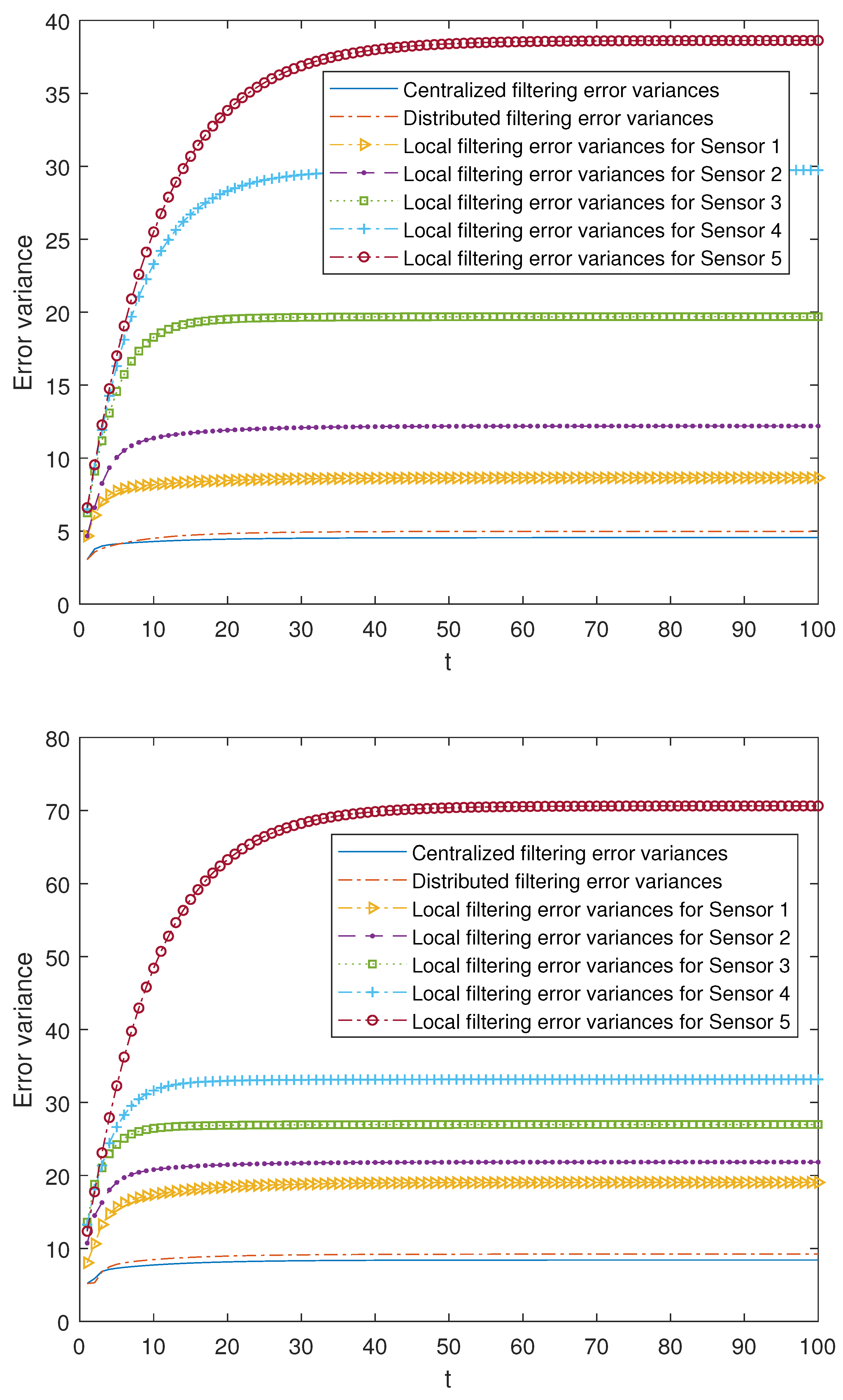
Firstly, taking fixed values for the probabilities $p_{j,\nu }^{\left(i\right)}$ for each of the ${\mathbb{T}}_k$-proper scenarios, the error variances of the local filters are compared with those of the centralized and distributed ones. These probabilities differ at each of the sensors, which allows us to make an initial attempt to contrast the three situations referred to the model, that is, the updated, delayed and uncertain observations. In this sense,

• In the ${\mathbb{T}}_1$-proper case:

  -

  Sensor 1: $p_1^{\left(1\right)}=0.9,p_2^{\left(1\right)}=0.05$,

  -

  Sensor 2: $p_1^{\left(2\right)}=0.7,p_2^{\left(2\right)}=0.05$,

  -

  Sensor 3: $p_1^{\left(3\right)}=0.05,p_2^{\left(3\right)}=0.9$,

  -

  Sensor 4: $p_1^{\left(4\right)}=0.05,p_2^{\left(4\right)}=0.7$,

  -

  Sensor 5: $p_1^{\left(5\right)}=p_2^{\left(5\right)}=0.05$.

• In the ${\mathbb{T}}_2$-proper case:

  -

  Sensor 1: $p_{1,r}^{\left(1\right)}=0.9$, $p_{1,{\eta }^{\prime }}^{\left(1\right)}=0.8$, $p_{2,r}^{\left(1\right)}=p_{2,{\eta }^{\prime }}^{\left(1\right)}=0.05$,

  -

  Sensor 2: $p_{1,r}^{\left(2\right)}=0.7$, $p_{1,{\eta }^{\prime }}^{\left(2\right)}=0.6$, $p_{2,r}^{\left(2\right)}=p_{2,{\eta }^{\prime }}^{\left(2\right)}=0.05$,

  -

  Sensor 3: $p_{1,r}^{\left(3\right)}=p_{1,{\eta }^{\prime }}^{\left(3\right)}=0.05$, $p_{2,r}^{\left(3\right)}=0.9$, $p_{2,{\eta }^{\prime }}^{\left(3\right)}=0.8$,

  -

  Sensor 4: $p_{1,r}^{\left(4\right)}=p_{1,{\eta }^{\prime }}^{\left(4\right)}=0.05$, $p_{2,r}^{\left(4\right)}=0.7$, $p_{2,{\eta }^{\prime }}^{\left(4\right)}=0.6$,

  -

  Sensor 5: $p_{j,\mu }^{\left(5\right)}=0.05$, for $j=1,2$ and $\mu =r,{\eta }^{\prime }$.

The results are displayed in Figure 1. The superiority of both centralized and distributed fusion filters over the local ones at each sensor can be observed, as well as the fact that these fusion filters have practically the same effectiveness, since their error variances are very close. Moreover, the local filtering error variances reflect the previously described three situations, considering the fact that the observations from sensors 1 and 2 are more conducive to being updated, those from sensors 3 and 4, delayed, and the most unfavorable case is for those from 5, since there exists a greater probability that they contain only noise. As before, the local error variances increase; then, the performance of the local filters becomes poorer as the situation of the updated, delayed and uncertain observations is more likely. Analogous results can be obtained by considering other different values of the Bernoulli parameters.

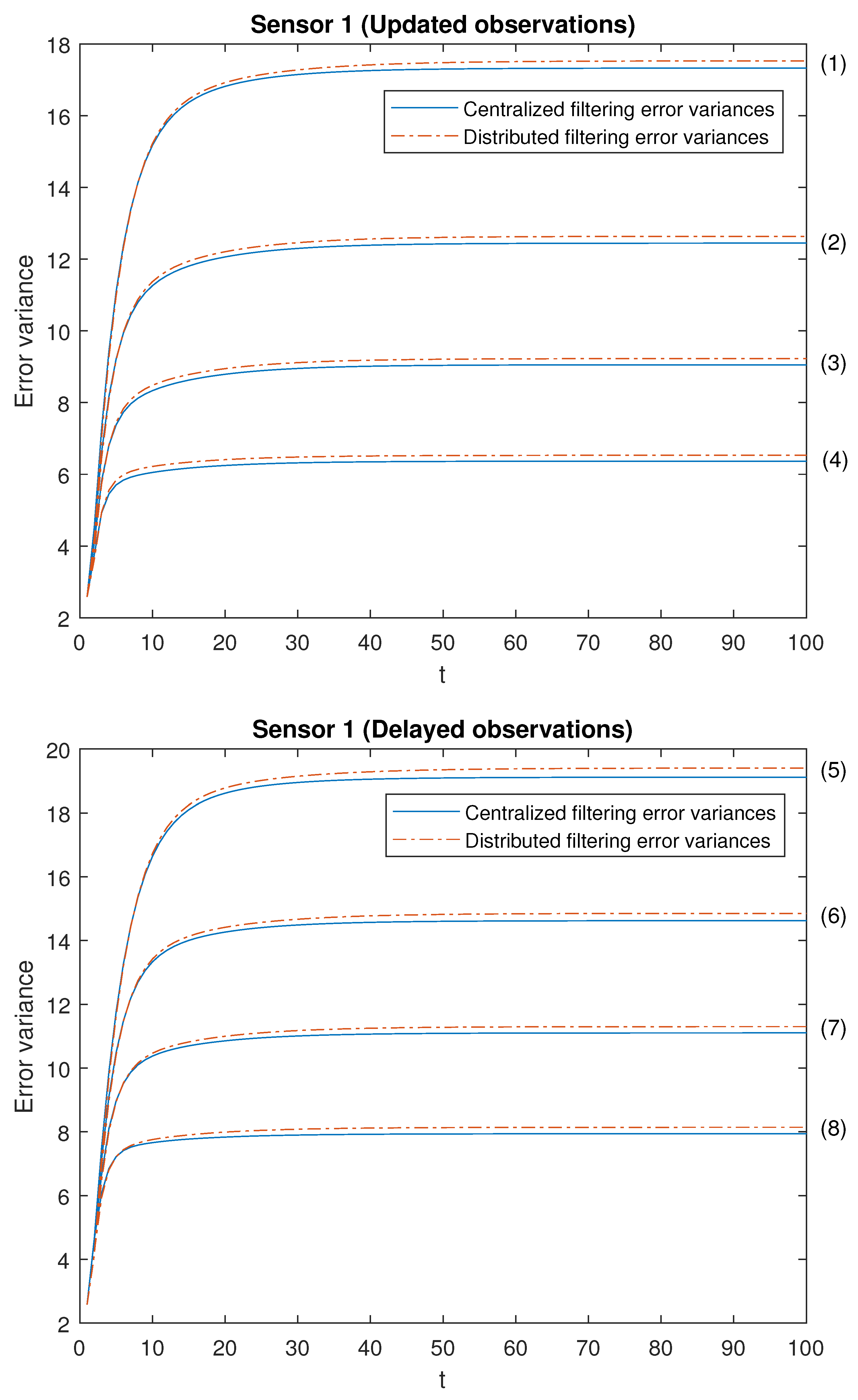
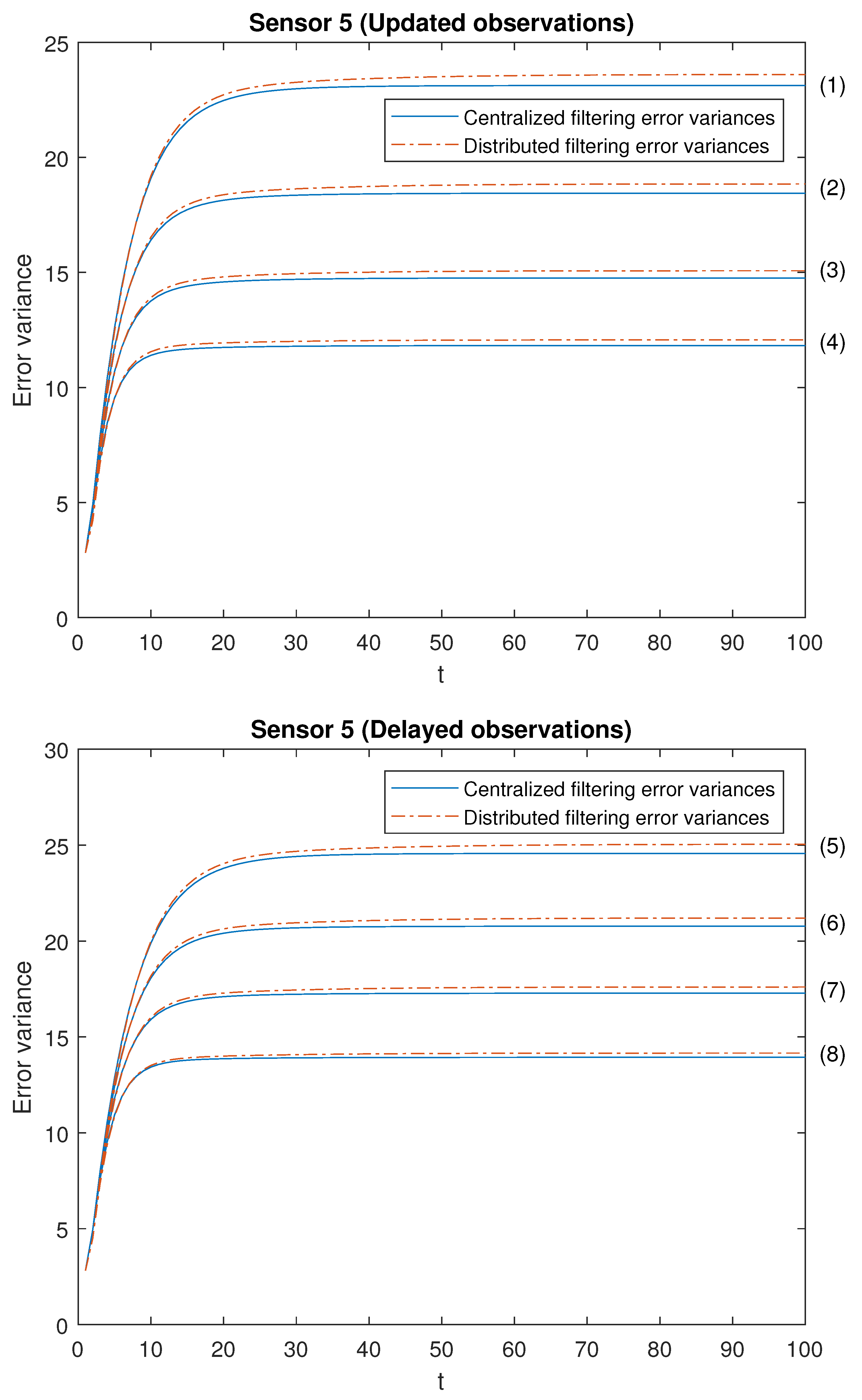
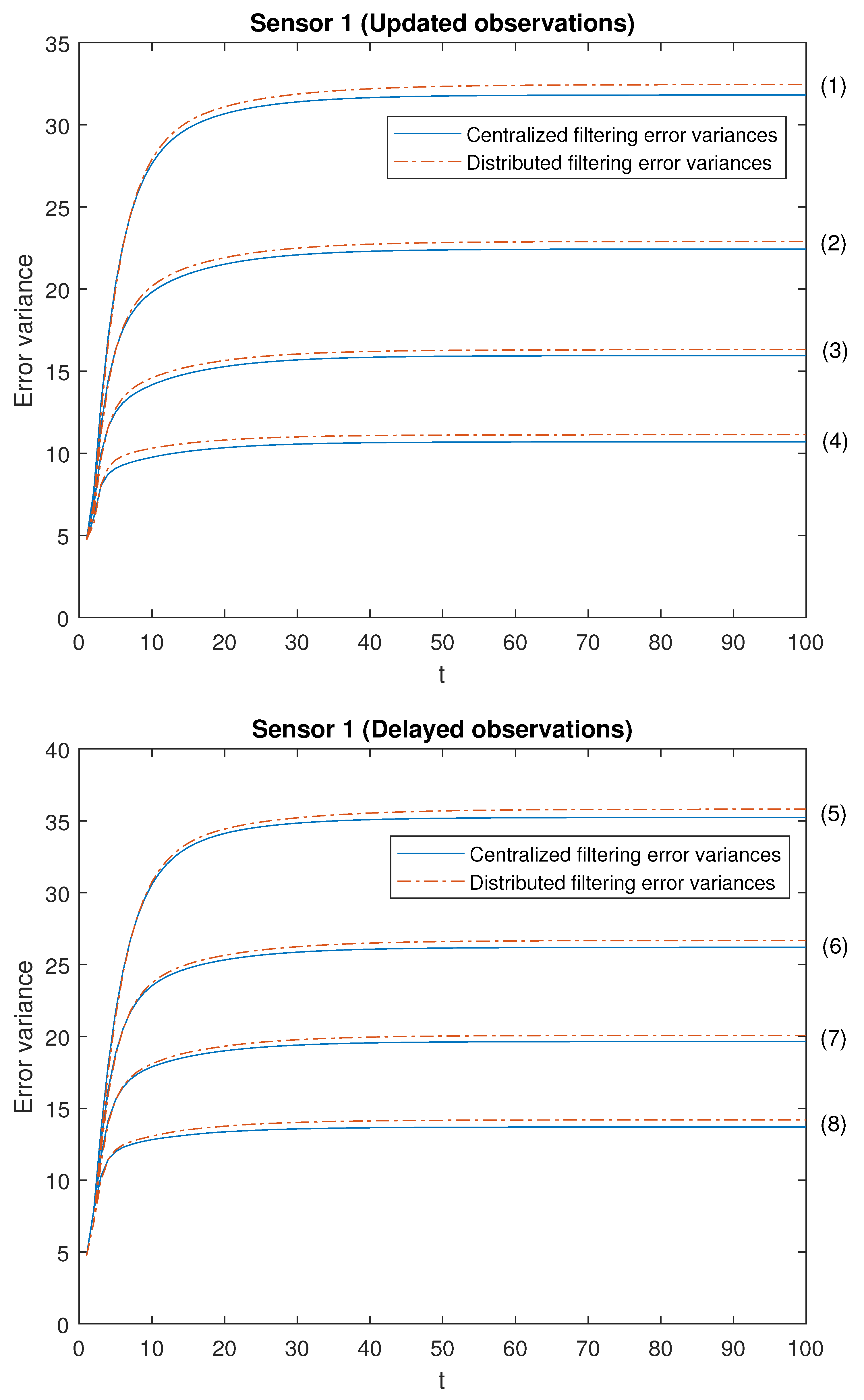
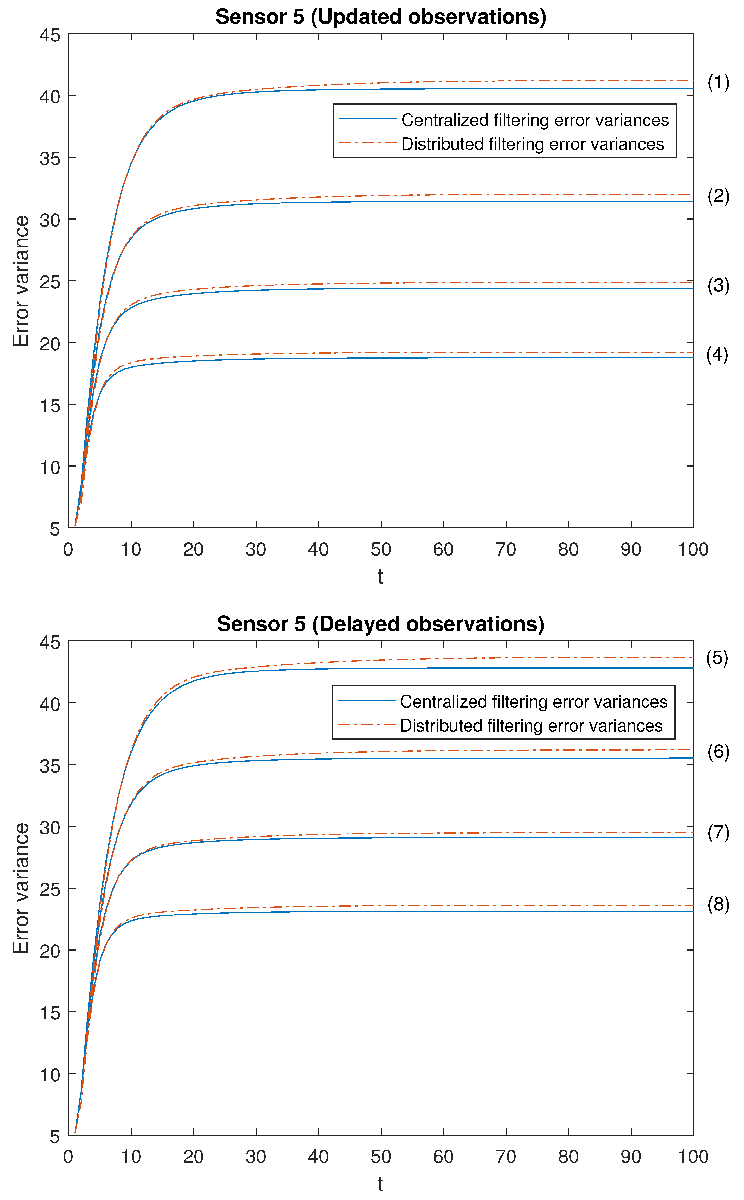
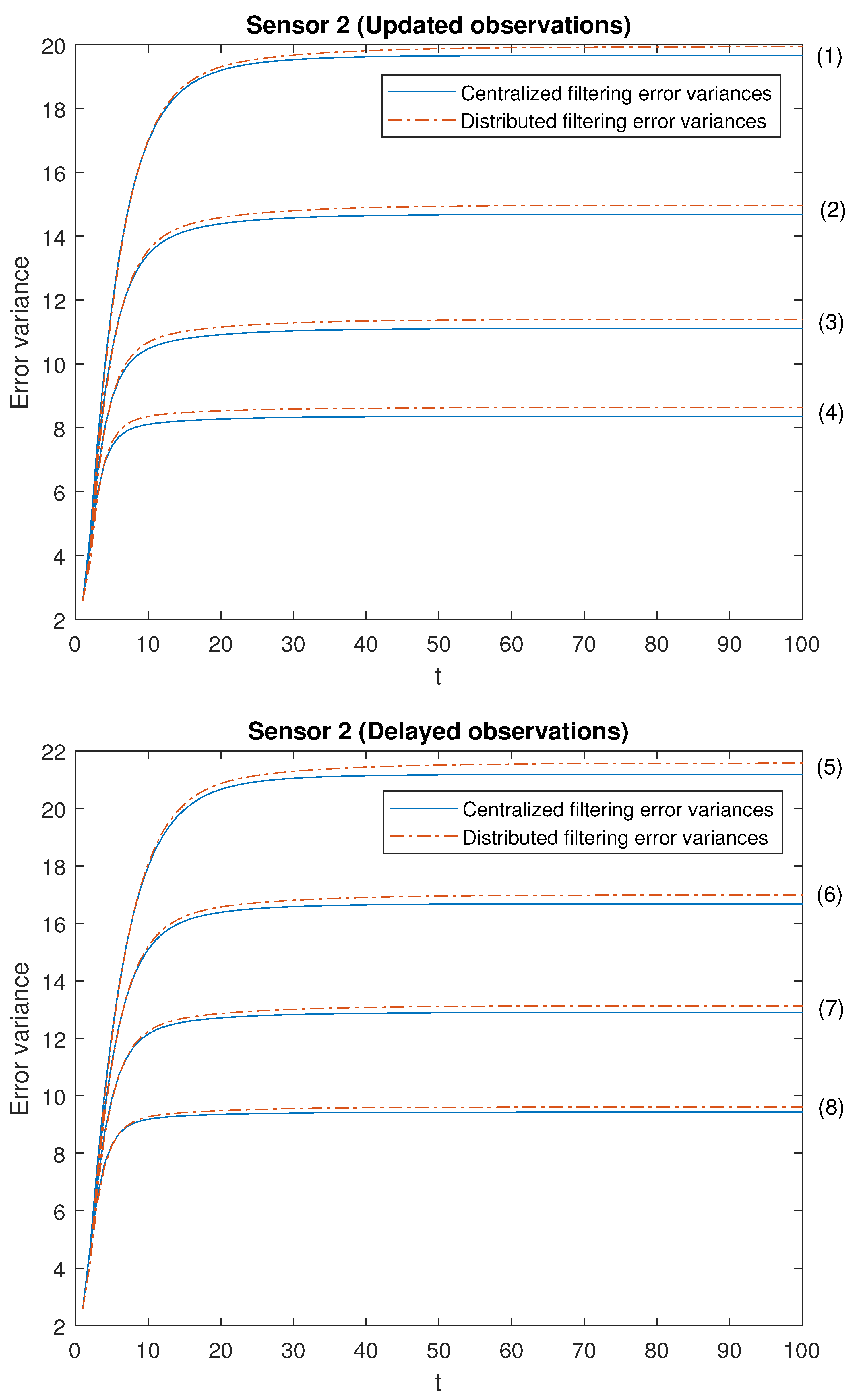
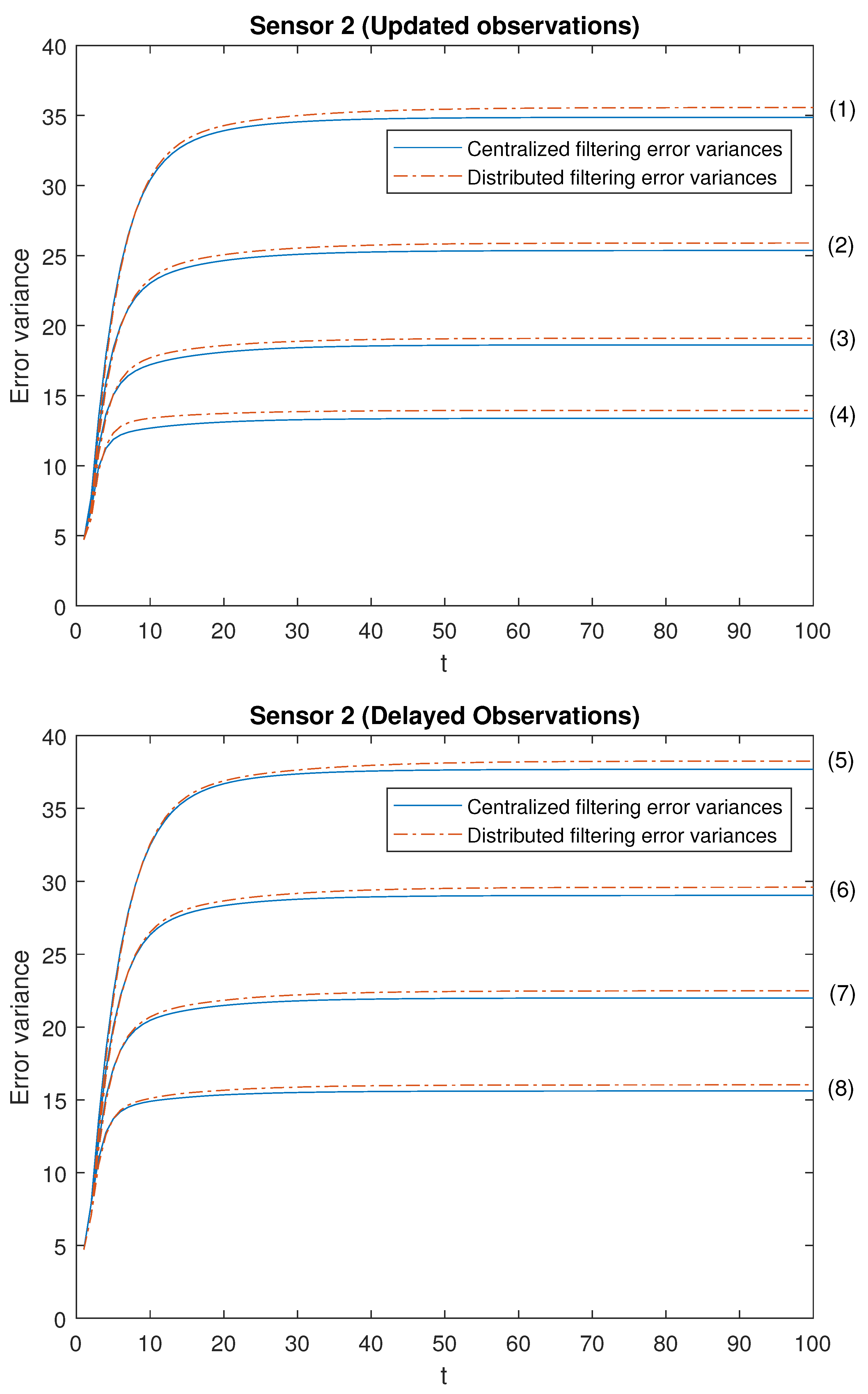
Our attention is focused on analyzing the accuracy of both centralized and distributed fusion filters in different situations concerning the observations produced by the sensors and in both ${\mathbb{T}}_k$-proper scenarios. For this purpose, we have considered the following cases with different values for the Bernoulli parameters:

• In the ${\mathbb{T}}_1$-proper scenario:

  -

  Cases in which updating probabilities vary at each sensor i:

  ∗

  (1): $p_1^{\left(i\right)}=0.3,p_2^{\left(i\right)}=0.05$, $p_j^{\left(l\right)}=0.05$, for $j=1,2$ and $l\ne i$;

  ∗

  (2): $p_1^{\left(i\right)}=0.5,p_2^{\left(i\right)}=0.05$, $p_j^{\left(l\right)}=0.05$, for $j=1,2$ and $l\ne i$;

  ∗

  (3): $p_1^{\left(i\right)}=0.7,p_2^{\left(i\right)}=0.05$, $p_j^{\left(l\right)}=0.05$, for $j=1,2$ and $l\ne i$;

  ∗

  (4): $p_1^{\left(i\right)}=0.9,p_2^{\left(i\right)}=0.05$, $p_j^{\left(l\right)}=0.05$, for $j=1,2$ and $l\ne i$;

  -

  Cases in which delay probabilities vary at each sensor i:

  ∗

  (5): $p_1^{\left(i\right)}=0.05,p_2^{\left(i\right)}=0.3$, $p_j^{\left(l\right)}=0.05$, for $j=1,2$ and $l\ne i$;

  ∗

  (6): $p_1^{\left(i\right)}=0.05,p_2^{\left(i\right)}=0.5$, $p_j^{\left(l\right)}=0.05$, for $j=1,2$ and $l\ne i$;

  ∗

  (7): $p_1^{\left(i\right)}=0.05,p_2^{\left(i\right)}=0.7$, $p_j^{\left(l\right)}=0.05$, for $j=1,2$ and $l\ne i$;

  ∗

  (8): $p_1^{\left(i\right)}=0.05,p_2^{\left(i\right)}=0.9$, $p_j^{\left(l\right)}=0.05$, for $j=1,2$ and $l\ne i$;

• In the ${\mathbb{T}}_2$-proper scenario:

  -

  Cases in which updating probabilities vary at each sensor i:

  ∗

  (1): $\left(p_{1,r}^{\left(i\right)},p_{1,{\eta }^{\prime }}^{\left(i\right)}\right)=(0.3,0.2)$, $p_{j,{\eta }^{\prime }}^{\left(l\right)}=p_{j,r}^{\left(l\right)}=0.05$, for $j=1,2$ and $l\ne i$;

  ∗

  (2): $\left(p_{1,r}^{\left(i\right)},p_{1,{\eta }^{\prime }}^{\left(i\right)}\right)=(0.5,0.4)$, $p_{j,{\eta }^{\prime }}^{\left(l\right)}=p_{j,r}^{\left(l\right)}=0.05$, for $j=1,2$ and $l\ne i$;

  ∗

  (3): $\left(p_{1,r}^{\left(i\right)},p_{1,{\eta }^{\prime }}^{\left(i\right)}\right)=(0.7,0.6)$, $p_{j,{\eta }^{\prime }}^{\left(l\right)}=p_{j,r}^{\left(l\right)}=0.05$, for $j=1,2$ and $l\ne i$;

  ∗

  (4): $\left(p_{1,r}^{\left(i\right)},p_{1,{\eta }^{\prime }}^{\left(i\right)}\right)=(0.9,0.8)$, $p_{j,{\eta }^{\prime }}^{\left(l\right)}=p_{j,r}^{\left(l\right)}=0.05$, for $j=1,2$ and $l\ne i$;

  -

  Cases in which delay probabilities vary at each sensor i:

  ∗

  (5): $\left(p_{2,r}^{\left(i\right)},p_{2,{\eta }^{\prime }}^{\left(i\right)}\right)=(0.3,0.2)$, $p_{j,{\eta }^{\prime }}^{\left(l\right)}=p_{j,r}^{\left(l\right)}=0.05$, for $j=1,2$ and $l\ne i$;

  ∗

  (6): $\left(p_{2,r}^{\left(i\right)},p_{2,{\eta }^{\prime }}^{\left(i\right)}\right)=(0.5,0.4)$, $p_{j,{\eta }^{\prime }}^{\left(l\right)}=p_{j,r}^{\left(l\right)}=0.05$, for $j=1,2$ and $l\ne i$;

  ∗

  (7): $\left(p_{2,r}^{\left(i\right)},p_{2,{\eta }^{\prime }}^{\left(i\right)}\right)=(0.7,0.6)$, $p_{j,{\eta }^{\prime }}^{\left(l\right)}=p_{j,r}^{\left(l\right)}=0.05$, for $j=1,2$ and $l\ne i$;

  ∗

  (8): $\left(p_{2,r}^{\left(i\right)},p_{2,{\eta }^{\prime }}^{\left(i\right)}\right)=(0.9,0.8)$, $p_{j,{\eta }^{\prime }}^{\left(l\right)}=p_{j,r}^{\left(l\right)}=0.05$, for $j=1,2$ and $l\ne i$;

Note that the cases (1)–(4) in both scenarios allow us to contrast the performance of the filters by varying the probability that the observations are updated. Moreover, the cases (1)–(4) are sorted in ascending order of the update probabilities. We will start with case (1), in which there exists a low probability that the observations are updated (that is, they will most probably contain only noise), and this probability increases until case (4), in which it is more likely that the available observations are the updated ones. Analogous consideration about delayed observations in cases (5)–(8). Note that (5) is the most favorable case regarding uncertain observations and (8) is the most unfavorable case regarding uncertain observations. The error variances of both centralized and distributed fusion filters in all the situations described above for sensors 1, 2 and 5, are displayed in Figure 2, Figure 3 and Figure 4, for the ${\mathbb{T}}_1$-proper scenario, and in Figure 5, Figure 6 and Figure 7, for the ${\mathbb{T}}_2$-proper one. In view of these figures, by first comparing the cases (1)–(4), it can be observed that the error variances of both fusion estimators decrease and, hence, the accuracy of the filters is better, as the probability that the observations at each sensor are updated increases. This is also true for cases (5)–(8), with delayed observations. Secondly, we compare, in both scenarios, the cases in pairs (1)–(5), (2)–(6), (3)–(7), (4)–(8). Note that each of these pairs represents the situations of updated and delayed observations with the same probability. From these figures, it can be observed that the error variances of the fusion filters are smaller when the observations are updated than when they are delayed. Finally, in all the cases and in both scenarios, these figures show that the filtering error variances of the centralized fusion estimators are lower than that of the distributed fusion ones, but the difference between them is insignificant, and this is even more acceptable in practice if we analyze the computational advantages of the calculus of the estimators by means of the distributed fusion filtering algorithm.

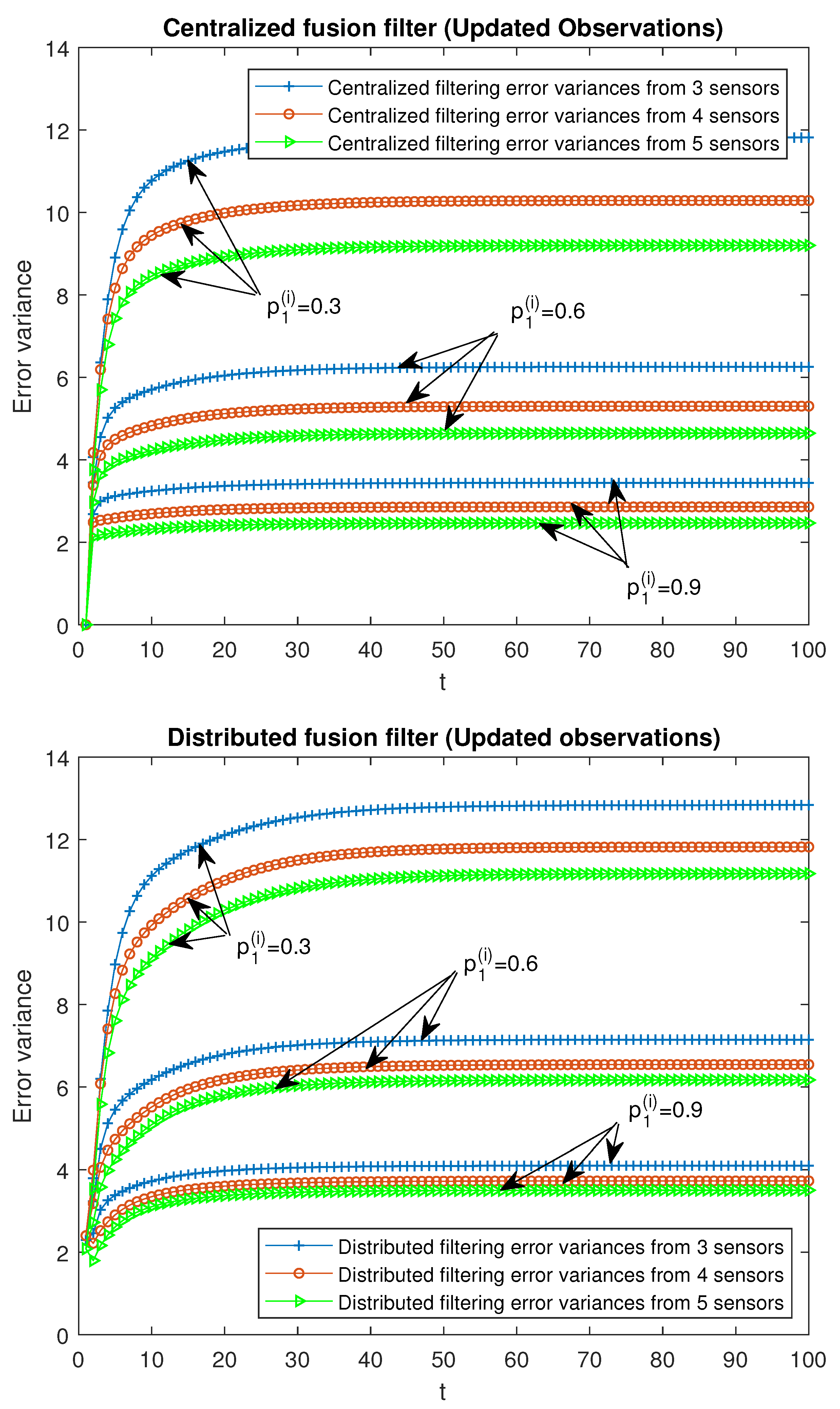
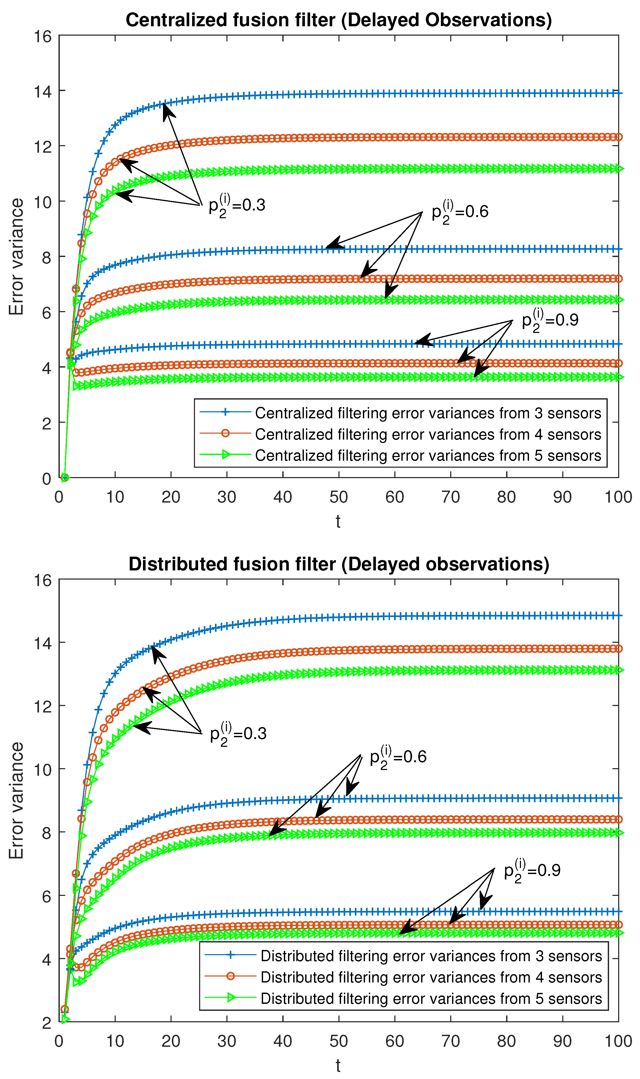
Finally, the performance of the proposed fusion filtering estimators is analyzed for different numbers of sensors, specifically, 3, 4 and 5 sensors in the ${\mathbb{T}}_1$-proper scenario. It is considered that the observations from all the sensors are modeled by the same observation equation; that is, they have the same updating or delay probabilities, as well as the same variance and covariance of the noises. For the case of updated observations, three situations were analyzed: $p_1^{\left(i\right)}=0.3,0.6,0.9$ for all $i=1,\dots ,5$, and the remaining ones, 0.05; another analogous situations for delayed observations: $p_2^{\left(i\right)}=0.3,0.6,0.9$ for all $i=1,\dots ,5$, and the remaining ones, 0.05. In Figure 8 and Figure 9, the ${\mathbb{T}}_1$-proper centralized and distributed fusion filtering error variances are displayed for the cases of updated and delayed observations, respectively. This was identitcal to that expressed in the above figures, but a better performance of both centralized and distributed filters was observed when the number of sensors increased.

8. Conclusions

In the last few decades, the scientific community has shown great interest in studying the signal estimation problem from multi-sensor observations, since better estimations are obtained with this method. The fact that there are several sensors reduces the number of possible failures in the communication channels as well as the adverse effects of some faulty sensors. Two methods have traditionally been used to build the fusion estimator from the observations of all the sensors: centralized and distributed methods. The first one has the advantage that it provides the optimal estimator whereas, with the distributed one, suboptimal estimators are obtained. However, the distributed method presents great advantages over the centralized one, such as flexibility, robustness, and a major reduction in the computational load (which is more significant with a large number of sensors), which make it preferable in practice, especially when considering the fact that in many real problems, the difference in performance between the estimators obtained by both methods may be almost insignificant.

The study of the signal estimation problem in hypercomplex domains has also considerably grown, since these domains allow for many real problems to be modeled in a better way. To date, most of the estimation problems have been addressed in the quaternion domain since it is a normed algebra. However, the tessarine signal processing can yield better estimators depending on the characteristics of the signal. Recently, it has been possible to endow the tessarine domain with a metric space structure that has the properties necessary to guarantee the existence and uniqueness of the orthogonal projection [41] which is a way of obtaining the LS linear estimator. Therefore, the signal estimation problem was addressed in the tessarine domain in different scenarios, and properness conditions were defined that are analogous to those existing in the quaternion domain. This obtained a considerable reduction in the augmented system, and it led to a consequent decrease in computational cost.

In this paper, under ${\mathbb{T}}_k$-properness conditions [41,42], the LS linear centralized and distributed fusion filtering problems of tessarine signals from multi-sensor observations have been studied, and recursive algorithms have been proposed to calculate them. The observations at each sensor and instant of time can be updated, delayed or contain only noise, independently from the other sensors. A correlation has also been assumed between the signal and observation noises. The ${\mathbb{T}}_k$-properness conditions cause an important computational reduction in the calculus of the ${\mathbb{T}}_k$-proper fusion filters in comparison with the TWL estimators, which makes these conditions desirable in practice. The theoretical results are illustrated in a numerical simulation example, in which the performance of the estimators calculated by using both fusion algorithms is compared by taking different values of the Bernoulli parameters modeling the updating, delay, or uncertainty in the observations.

Future research is planned to explore the signal estimation problem in other hypercomplex algebras, as well as to address the decentralized fusion estimation problem under ${\mathbb{T}}_k$-properness scenarios and different hypotheses on the observations.

References

1. Castanedo, F. A review of data fusion techniques. Sci. World. J. 2013, 2013, 704504. [Google Scholar] [CrossRef] [PubMed]
2. Fourati, H. Multisensor Data Fusion: From Algorithms and Architectural Design to Applications, 1st ed.; CRC Press, Taylor and Francis Group LLC: Boca Raton, FL, USA, 2015. [Google Scholar]
3. Sun, S.; Lin, H.; Ma, J.; Li, X. Multi-sensor distributed fusion estimation with applications in networked systems: A review paper. Inf. Fusion 2017, 38, 122–134. [Google Scholar] [CrossRef]
4. Abu Bakr, M.; Lee, S. Distributed multisensor data fusion under unknown correlation and data inconsistency. Sensors 2017, 17, 2472. [Google Scholar] [CrossRef] [Green Version]
5. Noack, B. State Estimation for Distributed Systems with Stochastic and Set-Membership Uncertainties; KIT Scientific Publishing: Karlsruhe, Germany, 2014. [Google Scholar]
6. He, S.; Shin, H.-S.; Xu, S.; Tsourdos, A. Distributed estimation over a low-cost sensor network: A review of state-of-the-art. Inf. Fusion 2020, 54, 21–43. [Google Scholar] [CrossRef]
7. Linares-Pérez, J.; Hermoso-Carazo, A.; Caballero-águila, R.; Jiménez-López, J.D. Least-squares linear filtering using observations coming from multiple sensors with one- or two-step random delay. Signal Process. 2009, 89, 2045–2052. [Google Scholar] [CrossRef]
8. Ma, J.; Sun, S. Centralized fusion estimators for multisensor systems with random sensor delays, multiple packet dropouts and uncertain observations. IEEE Sens. J. 2013, 13, 1228–1235. [Google Scholar] [CrossRef]
9. Liu, W.-Q.; Wang, X.-M.; Deng, Z.-L. Robust centralized and weighted measurement fusion Kalman estimators for uncertain multisensor systems with linearly correlated white noises. Inf. Fusion 2017, 35, 11–25. [Google Scholar] [CrossRef]
10. Liang, J.; Shen, B.; Dong, H.; Lam, J. Robust distributed state estimation for sensor networks with multiple stochastic communication delays. Int. J. Syst. Sci. 2011, 42, 1459–1471. [Google Scholar] [CrossRef]
11. Lin, H.; Sun, S. Distributed fusion estimator for multi-sensor asynchronous sampling systems with missing measurements. IET Signal Process. 2016, 10, 724–731. [Google Scholar] [CrossRef]
12. Sui, T.; Marelli, D.; Sun, X.; Fu, M. Multi-sensor state estimation over lossy channels using coded measurements. Automatica 2020, 111, 108561. [Google Scholar] [CrossRef]
13. Xing, Z.; Xia, Y.; Yan, L.; Lu, K.; Gong, Q. Multisensor distributed weighted Kalman filter fusion with network delays, stochastic uncertainties, autocorrelated, and cross-correlated noises. IEEE Trans. Syst. Man Cyber. Syst. 2018, 48, 716–726. [Google Scholar] [CrossRef]
14. Zhang, J.; Gao, S.; Li, G.; Xia, J.; Qi, X.; Gao, B. Distributed recursive filtering for multi-sensor networked systems with multi-step sensor delays, missing measurements and correlated noise. Signal Process. 2021, 181, 107868. [Google Scholar] [CrossRef]
15. Mo, Y.; Sinopoli, B. Kalman filtering with intermittent observations: Tail distribution and critical value. IEEE Trans. Autom. Control 2012, 57, 677–689. [Google Scholar]
16. Ihler, A.; Fisher III, J.W.; Willsky, A.S. Loopy belief propagation: Convergence and effects of message errors. J. Mach. Learn. Technol. 2005, 6, 905–936. [Google Scholar]
17. Duan, Y.; Zhang, X.; Li, Z. A new quaternion-based Kalman filter for human body motion tracking using the second estimator of the optimal quaternion algorithm and the joint angle constraint method with inertial and magnetic sensors. Sensors 2020, 20, 6018. [Google Scholar] [CrossRef]
18. Yao, Y.; Du, Z.; Huang, X.; Li, R. Derivation and simulation verification of the relationship between world coordinates and local coordinates under virtual reality engine. Virtual Real. 2020, 24, 263–269. [Google Scholar] [CrossRef]
19. Ortolani, F.; Comminiello, D.; Uncini, A. The widely linear block quaternion least mean square algorithm for fast computation in 3D audio systems. In Proceedings of the IEEE International Workshop on Machine Learning for Signal Processing (MLSP 2016), Salerno, Italy, 13–16 September 2016; p. 7738842. [Google Scholar]
20. Celsi, M.R.; Scardapane, S.; Comminiello, D. Quaternion neural networks for 3D sound source location in reverberant environments. In Proceedings of the IEEE International Workshop on Machine Learning for Signal Processing (MLSP 2020), Espoo, Finland, 21–24 September 2020; p. 9231809. [Google Scholar]
21. Grakhova, E.P.; Abdrakhmanova, G.I.; Schmidt, S.P.; Vinogradova, I.L.; Sultanov, A.K. The quadrature modulation of quaternion signals for capacity upgrade of high-speed fiber-optic wireless communication systems. In Proceedings of the SPIE—The Society for Optical Engineering, Munich, Germany, 23–27 June 2019; p. 11146. [Google Scholar]
22. Ahmad, Z.; Hashim, S.J.; Rokhani, F.Z.; Al-Haddad, S.A.R.; Sali, A.; Takei, K. Quaternion model of higher-order rotating polarization wave modulation for high data rate M2M LPWAN communication. Sensors 2021, 21, 383. [Google Scholar] [CrossRef]
23. Labunets, V.G. Hypercomplex models of multichannel images. Proc. Steklow Inst. 2021, 313, S155–S168. [Google Scholar] [CrossRef]
24. Augereau, B.; Carré, P. Hypercomplex polynomial wavelet-filter bank transform for color image. Signal Process. 2017, 136, 16–28. [Google Scholar] [CrossRef]
25. Mennano, G.M.; Mazzotti, A. Deconvolution of multicomponent seismis data by means of quaternions: Theory and preliminary results. Geophys. Prospect. 2012, 60, 217–238. [Google Scholar] [CrossRef]
26. Bahia, B.; Sacchi, M.D. Widely linear denoising of multicomponent seismic data. Geophys. Prospect. 2020, 68, 431–445. [Google Scholar] [CrossRef]
27. Takahashi, K.; Fujita, M.; Hashimoto, M. Remarks on octonion-valued neural networks with application to robot manipulator control. In Proceedings of the IEEE International Conference on Mechatronics (ICM 2021), Kashiva, Japan, 7–9 March 2021; p. 9385617. [Google Scholar]
28. Takahashi, K. Comparison of high-dimensional neural networks using hypercomplex numbers in a robot manipulator control. Artif. Life Robot. 2021, 26, 367–377. [Google Scholar] [CrossRef]
29. Dogic, Z.; Sharma, P.; Zakhary, M.J. Hypercomplex liquid crystals. Annu. Rev. Condens. Matter Phys. 2014, 5, 137–157. [Google Scholar] [CrossRef] [Green Version]
30. Ramírez-Tamayo, D.; Balcer, M.; Montoya, A.; Millwater, H. Mixed-mode stress intensity factors computation in functionally graded materials using a hypercomplex-variable finite element formulation. Int. J. Fract. 2020, 226, 219–232. [Google Scholar] [CrossRef]
31. Gao, Z.Y.; Niu, X.J.; Guo, M.F. Quaternion-based Kalman filter for micro-machined strapdown attitude heading reference system. Chin. J. Aeronaut. 2002, 15, 171–175. [Google Scholar] [CrossRef] [Green Version]
32. Martins, P.V.R.; Silva, O.M.; Lenzi, A. Insertion loss analysis of slender beams with periodic curvatures using quaternion-based parametrization, FE method and wave propagation approach. J. Sound Vib. 2019, 455, 82–95. [Google Scholar] [CrossRef]
33. Sabatelli, S.; Sechi, F.; Fanucci, L.; Rocchi, A. A sensor fusion algorithm for an integrated angular position estimation with inertial measurement units. In Proceedings of the Design, Automation and Test in Europe (DATE 2011), Grenoble, France, 14–18 March 2011; pp. 273–276. [Google Scholar]
34. Tannous, H.; Istrate, D.; Benlarbi-Delai, A.; Sarrazin, J.; Gamet, D.; Ho Ba Tho, M.C.; Dao, T.T. A new multi-sensor fusion scheme to improve the accuracy of knee flexion kinematics for functional rehabilitation movements. J. Sens. 2016, 16, 1914. [Google Scholar] [CrossRef] [Green Version]
35. Talebi, S.; Kanna, S.; Mandic, D. A distributed quaternion Kalman filter with applications to smart grid and target tracking. IEEE. Trans. Signal Inf. Process. Netw. 2016, 2, 477–488. [Google Scholar] [CrossRef]
36. Talebi, S.P.; Werner, S.; Mandic, D.P. Quaternion-valued distributed filtering and control. IEEE. Trans. Autom. Control 2020, 65, 4246–4256. [Google Scholar] [CrossRef]
37. Wu, J.; Zhou, Z.; Fourati, H.; Li, R.; Liu, M. Generalized linear quaternion complementary filter for attitude estimation from multi-sensor observations: An optimization approach. IEEE. Trans. Autom. Sci. Eng. 2019, 16, 1330–1343. [Google Scholar] [CrossRef]
38. Jiménez-López, J.D.; Fernández-Alcalá, R.M.; Navarro-Moreno, J.; Ruiz-Molina, J.C. Widely linear estimation of quaternion signals with intermittent observations. Signal Process. 2017, 136, 92–101. [Google Scholar] [CrossRef]
39. Fernández-Alcalá, R.M.; Navarro-Moreno, J.; Jiménez-López, J.D.; Ruiz-Molina, J.C. Semi-widely linear estimation algorithms of quaternion signals with missing observations and correlated noises. J. Frankl. Inst. 2020, 357, 3075–3096. [Google Scholar] [CrossRef]
40. Navarro-Moreno, J.; Fernández-Alcalá, R.M.; Jiménez-López, J.D.; Ruiz-Molina, J.C. Widely linear estimation for multisensor quaternion systems with mixed uncertainties in the observations. J. Frankl. Inst. 2019, 356, 3115–3138. [Google Scholar] [CrossRef]
41. Navarro-Moreno, J.; Fernández-Alcalá, R.M.; Jiménez-López, J.D.; Ruiz-Molina, J.C. Tessarine signal processing under the T-properness condition. J. Frankl. Inst. 2020, 357, 10099–10125. [Google Scholar] [CrossRef]
42. Navarro-Moreno, J.; Ruiz-Molina, J.C. Wide-sense Markov signals on the tessarine domain. A study under properness conditions. Signal Process. 2021, 183, 108022. [Google Scholar] [CrossRef]
43. Fernández-Alcalá, R.M.; Navarro-Moreno, J.; Ruiz-Molina, J.C. T-proper hypercomplex centralized fusion estimation for randomly multiple sensor delays systems with correlated noises. Sensors 2021, 21, 5729. [Google Scholar] [CrossRef] [PubMed]
44. Nitta, T.; Kobayashi, M.; Mandic, D.P. Hypercomplex widely linear estimation through the lens of underpinning geometry. IEEE Trans. Signal Process. 2019, 67, 3985–3994. [Google Scholar] [CrossRef]
Figure 1. Filtering error variances in the T 1 -proper scenario (top) and T 2 -proper one (bottom).
Mathematics 09 02961 g001
Figure 2. T 1 -proper fusion filtering error variances for updating probabilities: (1): p 1 ( 1 ) = 0.3 , p 2 ( 1 ) = 0.05 ; (2): p 1 ( 1 ) = 0.5 ,   p 2 ( 1 ) = 0.05 ; (3): p 1 ( 1 ) = 0.7 ,   p 2 ( 1 ) = 0.05 ; (4): p 1 ( 1 ) = 0.9 ,   p 2 ( 1 ) = 0.05 ; and delay probabilities: (5): p 1 ( 1 ) = 0.05 , p 2 ( 1 ) = 0.3 ; (6): p 1 ( 1 ) = 0.05 , p 2 ( 1 ) = 0.5 ; (7): p 1 ( 1 ) = 0.05 , p 2 ( 1 ) = 0.7 ; (8): p 1 ( 1 ) = 0.05 , p 2 ( 1 ) = 0.9 .
Mathematics 09 02961 g002
Figure 3. T 1 -proper fusion filtering error variances for updating probabilities: (1): p 1 ( 2 ) = 0.3 , p 2 ( 2 ) = 0.05 ; (2): p 1 ( 2 ) = 0.5 ,   p 2 ( 2 ) = 0.05 ; (3): p 1 ( 2 ) = 0.7 ,   p 2 ( 2 ) = 0.05 ; (4): p 1 ( 2 ) = 0.9 ,   p 2 ( 2 ) = 0.05 ; and delay probabilities: (5): p 1 ( 2 ) = 0.05 ,   p 2 ( 2 ) = 0.3 ; (6): p 1 ( 2 ) = 0.05 ,   p 2 ( 2 ) = 0.5 ; (7): p 1 ( 2 ) = 0.05 ,   p 2 ( 2 ) = 0.7 ; (8): p 1 ( 2 ) = 0.05 ,   p 2 ( 2 ) = 0.9 .
Mathematics 09 02961 g003
Figure 4. T 1 -proper fusion filtering error variances for updating probabilities: (1): p 1 ( 5 ) = 0.3 , p 2 ( 5 ) = 0.05 ; (2): p 1 ( 5 ) = 0.5 ,   p 2 ( 5 ) = 0.05 ; (3): p 1 ( 5 ) = 0.7 ,   p 2 ( 5 ) = 0.05 ; (4): p 1 ( 5 ) = 0.9 ,   p 2 ( 5 ) = 0.05 ; and delay probabilities: (5): p 1 ( 5 ) = 0.05 , p 2 ( 5 ) = 0.3 ; (6): p 1 ( 5 ) = 0.05 , p 2 ( 5 ) = 0.5 ; (7): p 1 ( 5 ) = 0.05 , p 2 ( 5 ) = 0.7 ; (8): p 1 ( 5 ) = 0.05 , p 2 ( 5 ) = 0.9 .
Mathematics 09 02961 g004
Figure 5. T 2 -proper fusion filtering error variances for updating probabilities: (1): p 1 , r ( 1 ) , p 1 , η ( 1 ) = ( 0.3 , 0.2 ) ; (2): p 1 , r ( 1 ) , p 1 , η ( 1 ) = ( 0.5 , 0.4 ) ; (3): p 1 , r ( 1 ) , p 1 , η ( 1 ) = ( 0.7 , 0.6 ) ; (4): p 1 , r ( 1 ) , p 1 , η ( 1 ) = ( 0.9 , 0.8 ) ; and delay probabilities: (5): p 2 , r ( 1 ) , p 2 , η ( 1 ) = ( 0.3 , 0.2 ) ; (6): p 2 , r ( 1 ) , p 2 , η ( 1 ) = ( 0.5 , 0.4 ) ; (7): p 2 , r ( 1 ) , p 2 , η ( 1 ) = ( 0.7 , 0.6 ) ; (8): p 2 , r ( 1 ) , p 2 , η ( 1 ) = ( 0.9 , 0.8 ) . In each case, the remaining probabilities are 0.05.
Mathematics 09 02961 g005
Figure 6. T 2 -proper fusion filtering error variances for updating probabilities: (1): p 1 , r ( 2 ) , p 1 , η ( 2 ) = ( 0.3 , 0.2 ) ; (2): p 1 , r ( 2 ) , p 1 , η ( 2 ) = ( 0.5 , 0.4 ) ; (3): p 1 , r ( 2 ) , p 1 , η ( 2 ) = ( 0.7 , 0.6 ) ; (4): p 1 , r ( 2 ) , p 1 , η ( 2 ) = ( 0.9 , 0.8 ) ; and delay probabilities: (5): p 2 , r ( 2 ) , p 2 , η ( 2 ) = ( 0.3 , 0.2 ) ; (6): p 2 , r ( 2 ) , p 2 , η ( 2 ) = ( 0.5 , 0.4 ) ; (7): p 2 , r ( 2 ) , p 2 , η ( 2 ) = ( 0.7 , 0.6 ) ; (8): p 2 , r ( 2 ) , p 2 , η ( 2 ) = ( 0.9 , 0.8 ) . In each case, the remaining probabilities are 0.05.
Mathematics 09 02961 g006
Figure 7. T 2 -proper fusion filtering error variances for updating probabilities: (1): p 1 , r ( 5 ) , p 1 , η ( 5 ) = ( 0.3 , 0.2 ) ; (2): p 1 , r ( 5 ) , p 1 , η ( 5 ) = ( 0.5 , 0.4 ) ; (3): p 1 , r ( 5 ) , p 1 , η ( 5 ) = ( 0.7 , 0.6 ) ; (4): p 1 , r ( 5 ) , p 1 , η ( 5 ) = ( 0.9 , 0.8 ) ; and delay probabilities: (5): p 2 , r ( 5 ) , p 2 , η ( 5 ) = ( 0.3 , 0.2 ) ; (6): p 2 , r ( 5 ) , p 2 , η ( 5 ) = ( 0.5 , 0.4 ) ; (7): p 2 , r ( 5 ) , p 2 , η ( 5 ) = ( 0.7 , 0.6 ) ; (8): p 2 , r ( 5 ) , p 2 , η ( 5 ) = ( 0.9 , 0.8 ) . In each case, the remaining probabilities are 0.05.
Mathematics 09 02961 g007
Figure 8. T 1 -proper fusion filtering error variances from updated observations with 3, 4 and 5 sensors.
Mathematics 09 02961 g008
Figure 9. T 1 -proper fusion filtering error variances from delayed observations with 3, 4 and 5 sensors.
Mathematics 09 02961 g009
Publisher’s Note: MDPI stays neutral with regard to jurisdictional claims in published maps and institutional affiliations.