Symmetry Preserving Discretization of the Hamiltonian Systems with Holonomic Constraints

Abstract

Symmetry preserving difference schemes approximating equations of Hamiltonian systems are presented in this paper. For holonomic systems in the Hamiltonian framework, the symmetrical operators are obtained by solving the determining equations of Lie symmetry with the Maple procedure. The difference type of symmetry preserving invariants are constructed based on the three points of the lattice and the characteristic equations. The difference scheme is constructed by using these discrete invariants. An example is presented to illustrate the applications of the results. The solutions of the invariant numerical schemes are compared to the noninvariant ones, the standard and the exact solutions.

1. Introduction

All variables are measured in a certain time interval, and all simulations can be implemented in meshes. Difference equations serve as primary and fundamental mathematical models in physics and mechanics. Symmetries concern the basic principles of physics and provide a most valuable heuristic guide in the search for dynamical laws. Continuous symmetries should be incorporated in the discretization of continuous systems, but they are usually lost in discrete descriptions [1,2].

Lie group theory is an efficient tool for solutions of differential equations [3]. It is also more convenient for the discretization of both ordinary differential equations (ODEs) [4,5,6] and partial differential equations (PDEs) [7,8,9]. For a given finite-difference equation (system), one can have the operators of the group admitted by the equation. Different types of difference equations which admit the different symmetry transformation operators can be obtained [10,11], and this theory is applied to search for discrete symmetries for dynamical systems [12,13]. Generally speaking, it needs to solve some linear partial finite-difference equations. But the problem of exact integration of partial finite-difference equations is always intractable, even when the equations are linear. Therefore, in order to construct the symmetry preserving difference schemes, the inverse problem needs to be solved, i.e., the difference equations and meshes are be constructed when the symmetries (transformation groups) are known. It is also a simpler way of having the symmetry preserving discretization of the differential equations.

It is better to keep the geometry structure during the discrete process. Payen, Matignon and Haine [14] addressed the discretization of the boundary controlled 3D Maxwell’s equations as a port-Hamiltonian system, and the proposed scheme preserves the Dirac structure at the discrete level. The symmetry structure is the geometry structure of the systems. It is meaningful to maintain the symmetry of the system in the discrete process. Verstappen and Veldman [15] studied the symmetry-preserving discretization of turbulent flow. Bourlioux, Rebelo and Winternitz [16] discretized the nonlinear ODEs under the group SL(2, R) using the symmetry preserving discretization method. The results showed that solution methods incorporating the Lie point symmetries provide better results than standard methods. The symmetry preserving schemes not only serve as fundamental mathematical models but also preserve main geometric properties of the dynamical systems [17,18]. Dorodnitsyn et al. proposed approaches on the applications of Lie group theory to difference equations and discrete mechanical systems [19]. This approach is to start with a differential equation and to introduce a symmetry adapted mesh and difference equation in such a way that all the symmetries of the original differential equation are preserved [20]. Levi’s [21], Winternitz’s [22], and Rebelo’s [23] contributions are the typical representatives for this approach.

There have been some papers on constructing the invariant discretizations of dynamical systems based on the inverse problem method above, such as the one-dimensional gas systems [24], the shallow water equations in Lagrangian [25], the holonomic dynamical systems [23], etc. The symmetry preserving discretization of ODE and PDE are studied deeply [9,10,19,20,21,22,23]. The theory has been applied to dynamical systems recently. The references [7,12,18,24,25,26] studied symmetry preserving schemes in a Lagrangian framework. In the Lagragian framework, the symmetry-preserving structure is studied in the space $M=Q\times ℝ$ or $M=TQ\times ℝ$. The transformation group $\psi : M\to M$. The Lie transformation generators are ${\tau }_{\alpha },{\xi }_{\alpha }^{\mu },{\eta }_{\alpha }^{\mu }: M\to ℝ$. In this paper, the symmetry-preserving structure is in the dual space $M=T^{\ast }Q\times ℝ$ of the tangent space. The conditions of preserving the symmetries of the Hamiltonian systems are studied, and the corresponding numerical simulation are proposed. The goal of this article is to extend the method of invariant discretization of differential equations to the holonomic Hamiltonian systems. This new method can preserve fundamental symmetric properties and improve the features of numerical algorithms in a Hamiltonian framework. The main goal of this paper is to find a way to discretize the constrained systems in the Hamiltonian framework. Generally speaking, the constrained dynamical systems are universal in engineering but relatively difficult in terms of getting a solution. Suppose the systems are subject to holonomic constraint. Although it is simpler, the results could make some preliminary analysis in the numerical simulation of complex systems.

The paper is structured as follows. In Section 2, the Lie symmetry of Hamiltonian systems with holonomic constraints are recalled, based on the infinitesimal generators and the prolongations. In Section 3, the Lie point symmetry group in Section 2 is prolonged to the three points of lattice, and the invariant difference scheme is obtained by solving the discrete characteristic equations. The symmetry preserving discretization of the Hamiltonian systems with holonomic constraints are constructed by the difference invariants. Section 4 is devoted to an example to illustrate the theoretical results, and the Hamiltonian system’s behaviors are simulated using the invariant discretization. Some conclusions are drawn in Section 5. Throughout the paper Einstein’s summation is used.

2. Lie Symmetry of Hamiltonian Systems with Holonomic Constraints

2.1. The Equations of the Constrained Hamiltonian System

Let $X={ℝ}^m$ be the space representing the independent variables, and $U={ℝ}^n$ represent the dependent variables. Consider a mechanical system whose configuration is determined by n generalised coordinates $q_s(s=1, \dots , n)$. Let the motion of the system be subjected to the g holonomic constraints $Q_s=Q_s\left(t, q_s, {\dot{q}}_s\right)$, the differential equations of motion of the system can be written in the form

$$\frac{\mathrm{d}}{\mathrm{d}t}\frac{\partial L}{\partial {\dot{q}}_s}-\frac{\partial L}{\partial q_s}=Q_s,$$

(1)

where $L=L(t, q_s, {\dot{q}}_s)$ is the Lagrangian, $Q_s$ are the non-potential generalised forces. Introduce the generalized momentum and Hamilton function

$$p_s=\frac{\partial L}{\partial {\dot{q}}_s}, H=p_s{\dot{q}}_s-L,$$

(2)

and the canonical form of equations of the Hamiltonian systems with holonomic constraints are

$$F_1={\dot{q}}_s-{\partial }_{p_s}H=0, F_2={\dot{p}}_s+{\partial }_{q_s}H-{\overline{Q}}_s=0,$$

(3)

involving one independent variables t and 2n dependent variables $p_s=(p_1, \dots , p_n)$ and $q_s=(q_1, \dots , q_n)$ where ${\partial }_{q_s}=\partial /\partial q_s, {\partial }_{p_s}=\partial /\partial p_s$, H is the Hamiltonian, ${\overline{Q}}_s$ are the nonpotential generalized forces as functions of $t, q_s$ and $p_s$. Expanding Equation (3), we can solve ${\dot{q}}_s$ and ${\dot{p}}_s$ as

$${\dot{q}}_s=g_s(t, p_s, q_s), {\dot{p}}_s=h_s(t, p_s, q_s).$$

(4)

2.2. Infnitesimal Generators and the Prolongations

A symmetry group of the system will be a local group of transformation G_r in Z acting on the open subset $M\subset X\times U$. For the holonomic Hamiltonian systems with $X=ℝ$ and $U={ℝ}^{2n}$, we denote a local one parameter continuous transformation group G₁ concerning t, q_s and p_s to a continuous parameter $\epsilon \in {ℝ}^{2n}$ can be taken from

$$t^{\ast }=\varphi (t, p_s, q_s, \epsilon ), q_s^{\ast }(t^{\ast })=\phi (t, p_s, q_s, \epsilon ), p_s^{\ast }(t^{\ast })=\psi (t, p_s, q_s, \epsilon ).$$

(5)

Accordingly, the transformations in the group G₁ acting on the variables can be written as

$$t^{*}=t+\epsilon \left(\frac{\partial \varphi }{\partial \epsilon }\left|{}_{\epsilon \to 0}\right.\right)+ O({\epsilon }^2), q_s^{*}=q_s+\epsilon \left(\frac{\partial \phi }{\partial \epsilon }\left|{}_{\epsilon \to 0}\right.\right)+ O({\epsilon }^2), p_s^{*}=p_s+\epsilon \left(\frac{\partial \psi }{\partial \epsilon }\left|{}_{\epsilon \to 0}\right.\right)+ O({\epsilon }^2),$$

(6)

since ε→0 forms the identity of the group. The infinitesimals are defined by the new functions:

$$\tau (t,p_s,q_s)=\frac{\partial \varphi }{\partial \epsilon }\left|{}_{\epsilon \to 0}, {\xi }_s(t,p_s,q_s)=\right.\frac{\partial \phi }{\partial \epsilon }\left|{}_{\epsilon \to 0}, {\eta }_s\right.(t,p_s,q_s)=\frac{\partial \psi }{\partial \epsilon }\left|{}_{\epsilon \to 0}.\right.$$

Then, Equation (5) becomes

$$t^{\ast }=t+\epsilon \tau (t, p_s, q_s), q_s^{\ast }=q_s+\epsilon {\xi }_s(t, p_s, q_s), p_s^{\ast }=p_s+\epsilon {\eta }_s(t, p_s, q_s).$$

(7)

The first prolongation of the infinitesimal generators should also be known for the Hamiltonian systems with holonomic constraints. By obtaining ${\dot{q}}_s^{\ast }$ and ${\dot{p}}_s^{\ast }$:

$$\begin{gathered} {\dot{q}}_s^{\ast }=\frac{d{q}_s^{\ast }}{d{t}^{\ast }}=\frac{q_s^{\ast }+\epsilon D_t({\xi }_s)}{1+D_t(\tau )}={\dot{q}}_s-{\dot{q}}_s\epsilon D_t(\tau )+\epsilon D_t({\xi }_s)-{\epsilon }^2{D}_t({\xi }_s)D_t(\tau ), \\ {\dot{q}}_s^{\ast }=\frac{d{q}_s^{\ast }}{d{t}^{\ast }}=\frac{q_s^{\ast }+\epsilon D_t({\xi }_s)}{1+D_t(\tau )}={\dot{q}}_s-{\dot{q}}_s\epsilon D_t(\tau )+\epsilon D_t({\xi }_s)-{\epsilon }^2{D}_t({\xi }_s)D_t(\tau ), \end{gathered}$$

where D_t is the total derivative operator for time. Ignoring the high-order terms, we have

$$q_s^{\ast }={\dot{q}}_s+\epsilon (D_t({\xi }_s)-{\dot{q}}_s{D}_t(\tau )), p_s^{\ast }={\dot{p}}_s+\epsilon (D_t({\eta }_s)-{\dot{p}}_s{D}_t(\tau ))$$

One can determine the tangent vector field γ = {τ, ξ_s, η_s}^T, of the group at the point (t, q_s, p_s), where τ, ξ_s and η_s are unknown and demand to be determined to achieve the symmetry transformation. The Lie algebra L of the symmetry group G₁ is realized by vector fields of the form

$$X_s^{(0)}=\tau {\partial }_t+{\xi }_s{\partial }_{q_s}+{\eta }_s{\partial }_{p_s},$$

(8)

and the first prolongation is

$$X_s^{(1)}=X_s^{(0)}+(D_t({\xi }_s)-{\dot{q}}_s{D}_t(\tau )){\partial }_{{\dot{q}}_s}+(D_t({\eta }_s)-{\dot{p}}_s{D}_t(\tau )){\partial }_{p_s},$$

(9)

where ${\partial }_t=\partial /\partial t$.

In the same way, the vector fields and the prolongation of systems (1) in Lagrangian framework are

$$X_s^{(0)}=\tau {\partial }_t+{\xi }_s{\partial }_{q_s},$$

(10)

$$X_s^{(1)}=X_s^{(0)}+(D_t({\xi }_s)-{\dot{q}}_s{D}_t(\tau )){\partial }_{{\dot{q}}_s},$$

(11)

$$X_s^{(2)}=X_s^{(1)}+(D_t({\xi }_s)-{\dot{q}}_s{D}_t(\tau )){\partial }_{{\dot{q}}_s}+({\ddot{\xi }}_s-2{\ddot{q}}_s{\dot{\xi }}_0+{\dot{q}}_s{\ddot{\xi }}_0){\partial }_{{\ddot{q}}_s}.$$

(12)

2.3. Lie Symmetries for Hamiltonian Systems

The algorithm for finding the symmetry algebra and the symmetry group for a given Equation (3) goes back to S. Lie and is given in many books on the subject [3]. For the equations of Hamiltonian systems, the symmetry algebra L and the symmetry group G₁ are given as follows.

Definition 1.

If G₁ is a local group of transformations acting on M, and

$$X_s^{(1)}(F_{\sigma })\left|{}_{F_{\sigma =0}}=0, \sigma =1,2\right.,$$

(13)

for every infinitesimal generator of G₁, then G₁ is a Lie symmetry group of the systems.

Considering Equation (4), the determining equations of the Lie symmetries for Equation (3) under the transformation (8) have the form

$$D_t({\xi }_s)-g_s{D}_t(\tau )=X_s^{(0)}(g_s),D_t({\eta }_s)-h_s{D}_t(\tau )=X_s^{(0)}(h_s),$$

(14)

where $g_s={\partial }_{p_s}H$ and $h_s=-{\partial }_{q_s}H+{\overline{Q}}_s$. This produces 2n partial differential equations to determine the functions τ, ξ_s and η_s. These equations provide an effective computational procedure for finding the most general symmetry group of the systems. In this procedure, the coefficients τ, ξ_s and η_s of the infinitesimal transformation generator $X_s^{(0)}$ of one-parameter symmetry group of the systems be unknown functions of t, q_s and p_s. The determining Equations (14) will thus involve t, q_s and p_s, as well as τ, ξ_s, η_s and their partial derivatives with respect to t, q_s and p_s. We can equate the coefficients of the remaining derivative of q_s and p_s to zero after eliminating any dependencies among the derivative of the q_s’s and p_s’s caused by the system itself. This will result in solving a large number for the coefficient functions τ, ξ_s and η_s for the infinitesimal generator. In most instances, these determining equations can be solved by elementary method, and the general solution will determine the most general infinitesimal symmetry of the system.

We can also use an existing software program designed to automate the major steps of this algorithm in order to calculate the symmetry group of the system more efficiently, such as Mathematica [27], Maple [28], etc. In this paper, the symmetry operators are obtained in Maple. In general, the Low-order differential equations can be solved by the determine() provided by liesymm, an embedded software package in Maple system [29]. The solution of symmetric equations of higher order nonlinear partial differential equations can be obtained by means of some standard software packages like PDEtools [30], SADE [31], GeM [32], etc.

3. The Lie Symmetry-Preserving Difference Scheme for Hamiltonian Systems with Holonomic Constraints

3.1. Invariance of Difference Equations of Hamiltonian Systems

Consider the space Z of sequences (t, q_s, p_s), and denote by D the first order linear discrete operator

$$D=\frac{\partial }{\partial t}+{\dot{q}}_s\frac{\partial }{\partial q_s}+{\dot{p}}_s\frac{\partial }{\partial p_s}+\dots$$

Fixing arbitrary parameter value h > 0, we form a pair of the operators of discrete transformation to the right and left

$$\underset{+h}{S}=e^{hD}=\frac{h^m}{m!}{D}^m,\underset{-h}{S}=e^{-hD}=\frac{{(-h)}^m}{m!}{D}^m,$$

where D is a derivation in Z. The operators $\underset{+h}{S}$ and $\underset{-h}{S}$ commute with each other and satisfy $\underset{+h}{S}\underset{-h}{S}=\underset{-h}{S}\underset{+h}{S}=1$.

Consider Hamiltonian difference equations at some lattice points (t, q_s and p_s). Generally, the lattice is irregular.

Using $\underset{+h}{S}$ and $\underset{-h}{S}$ we define a pair of right and left discrete (finite-difference) differentiation operators by setting

$$\underset{+h}{D}=\frac{\underset{+h}{S}-1}{h}\equiv \frac{h^{m-1}}{m!}{D}^m,\underset{-h}{D}=\frac{1-\underset{-h}{S}}{h}\equiv \frac{{(-h)}^{m-1}}{m!}{D}^m,$$

where $\underset{\pm h}{D}$ denote total difference derivatives in the time directions with steps h. The operators $\underset{+h}{S}, \underset{-h}{S}, \underset{+h}{D}$ and $\underset{-h}{D}$ commute in any combination, while $\underset{-h}{D}=\underset{+h}{D}\underset{-h}{S},\underset{+h}{D}=\underset{-h}{D}\underset{+h}{S}$. The shift operators $\underset{\pm h}{S}$ and the discrete differentiation operators $\underset{\pm h}{D}$ introduce new variables (the difference derivatives and the lattice) while discretizing the space Z.

Let $\underset{h}{Z}$ be the space of sequences of mesh variables $\left(t, q_i, p_i, q_{i,t}, p_{i,t}, h^{+}, h^{-}\right)$ and let $\underset{h}{A}$ the space of analytic functions of finitely many coordinates z_i of a vector $\underset{h}{Z}$. We introduce the one-dimensional difference mesh t⁺ = t + h⁺ and $h^{+}\in \underset{h}{\omega }$. Then each finite-difference equations on the mesh $\underset{h}{\omega }$ can be written as

$$F_1^d=q_{i,t}-{\partial }_{p_i^{+}}H=0, F_2^d=p_{i,t}+{\partial }_{q_i}H-{\overline{Q}}_i=0, i=1,\dots n,$$

(15)

where $F_{\sigma }^d\in \underset{h}{A}$, $q_{i,t}=\underset{+h}{D}\left(q_i\right)=\left(q_i^{+}-q_i\right)/h^{+}$, $p_{i,t}=\underset{+h}{D}\left(p_i\right)=\left(p_i^{+}-p_i\right)/h^{+}$. This equation is writ ten on finitely many points of the difference mesh $\underset{h}{\omega }$. We assume that the mesh is determined by the equation

$${\Omega }_{\beta (z)}=0, \beta =1,\dots ,m,$$

(16)

where $\Omega \in \underset{h}{A}$. The function Ω is uniquely determined by the discretization of the space of independent variables. In the continuous limit one equation, the Equation (16) reduces to an identity (like 0 = 0).

The vector fields are the same as in the continuous case, however they must be prolonged to all points of the lattice, involved in the system (15) and (16). We have G₁ be a one-parameter group in Z with operator

$$pr{X}_i^{(1)}=\tau {\partial }_t+{\xi }_i{\partial }_{q_i}+{\eta }_i{\partial }_{p_i}+{\xi }_i^t{\partial }_{q_{i,t}}+{\eta }_i^t{\partial }_{p_{i,t}}+({\tau }^{+}-\tau ){\partial }_{h^{+}}+(\tau -{\tau }^{-}){\partial }_{h^{-}},$$

(17)

where ${\xi }_i^t=\underset{+h}{D}({\xi }_i)-q_{i,t}\underset{+h}{D}(\tau )$ and ${\eta }_i^t=\underset{+h}{D}({\eta }_i)-p_{i,t}\underset{+h}{D}(\tau )$.

Definition 2.

For the difference Equation (15) to admit the group with operator (17) on the mesh (16), if the infinitesimal generators τ, ξ_i and η_i satisfy the determining equations

$$pr{X}_i^{(1)}(F_{\sigma }^d(z))\left|{}_{F_{\sigma }^d(z)=0,{\Omega }_{\beta (z)=0}}=0,\right.$$

(18)

$$pr{X}_i^{(1)}({\Omega }_{\beta }(z))\left|{}_{F_{\sigma }^d(z)=0,{\Omega }_{\beta (z)=0}}=0,\right.$$

(19)

then the symmetry is the Lie symmetry of discrete Hamiltonian systems with holonomic constraint.

The mesh spacing transformations are $h^{+}$ and $h^{-}$. By using the uniform mesh $h^{+}=h^{-}$ and applying the infinitesimal transformation (7), we obtain $pr{X}_i^{(1)}\left(h^{+}\right)=pr{X}_i^{(1)}\left(h^{-}\right)$, the coordinate τ of the operator(17) satisfy ${\tau }^{+}-\tau =\tau -{\tau }^{-}$ or $\underset{+h}{D}\underset{+h}{D}\left(\tau \right)=0$. Thus, we have the following proposition.

Proposition 1.

For the mesh$\underset{h}{\omega }$to remain uniform under the action of the transformation group G₁ of the Hamiltonian systems, it is necessary and sufficient that the following condition be satisfied at each point:

$$\underset{+h}{D}\underset{-h}{D}(\tau (z))=0.$$

(20)

The meshes satisfying (20) are said to be invariantly uniform for the systems.

3.2. The Lie Symmetry-Preserving Difference Scheme for Hamiltonian Systems

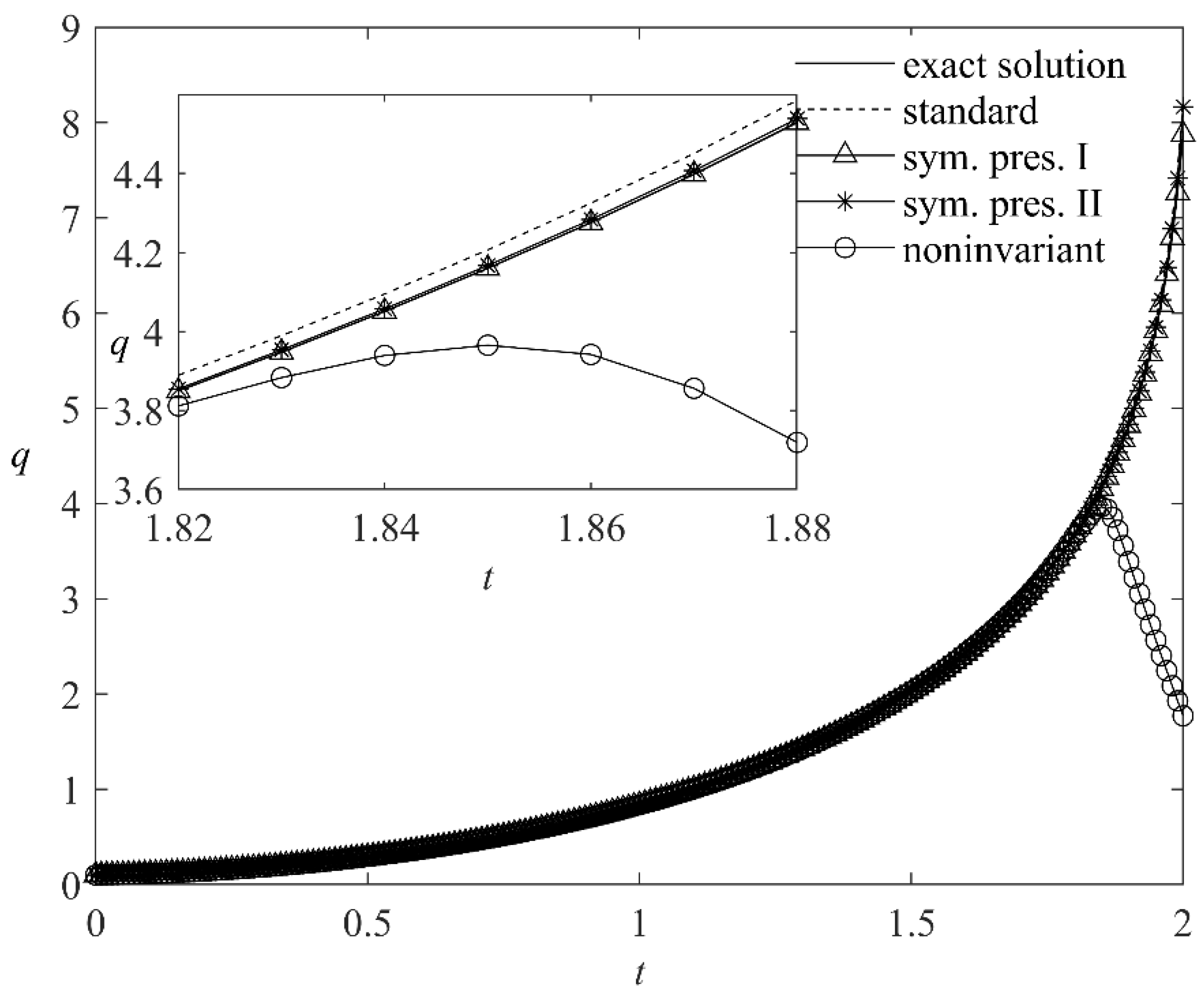
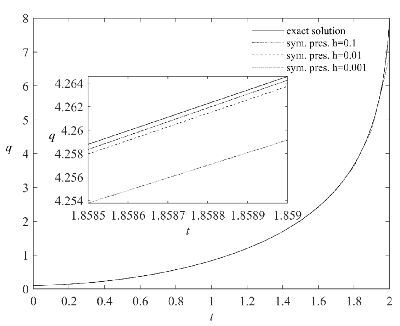
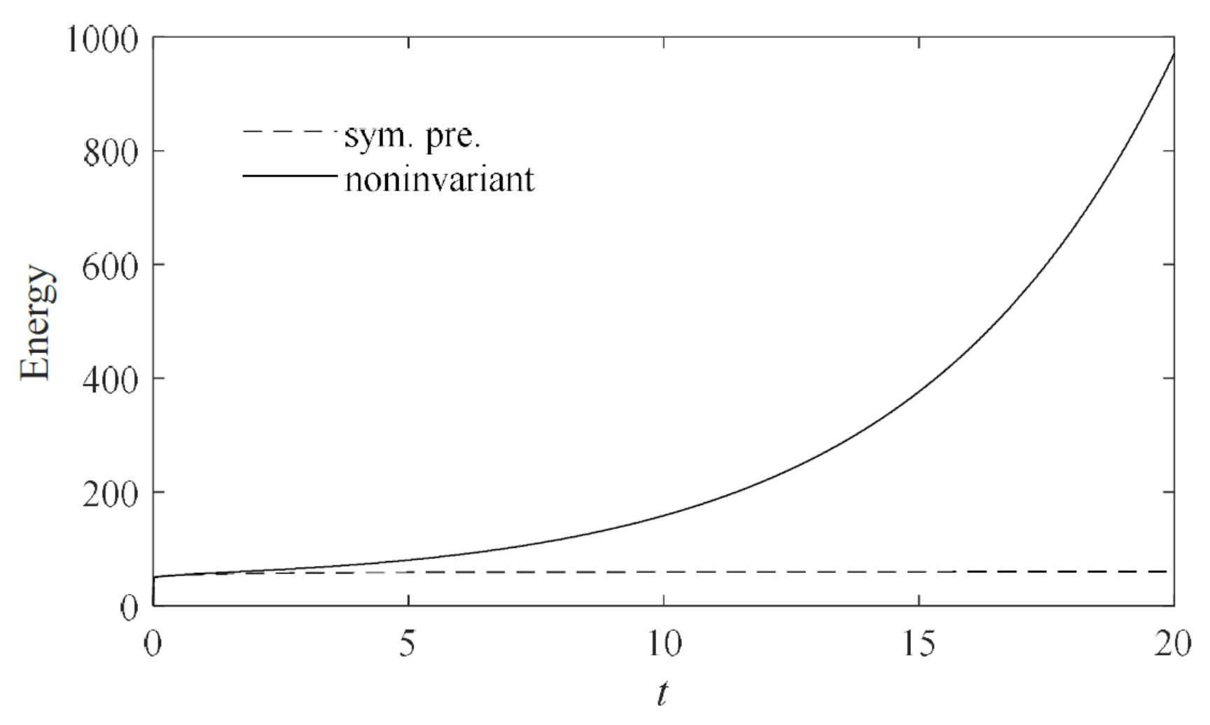
Suppose the Hamiltonian Equation (3) admit a known transformation group G₁ without loss of generality, after the complete set of r functionally independent invariants $(I_1^C(z), \dots , I_r^C(z))$ of order k is constructed, system(3) can be rewritten in the invariant representation ${\Psi }_a(I_1^C(z), \dots , I_r^C(z))=0$.

For the systems of the difference Equation (15) and the difference mesh (16) which admits the same group G₁ and provide a first order approximation to the original systems (3). We wish to construct the difference scheme that not only approximates Equation (3), but has the same Lie point symmetry group G₁. This is achieved by constructing the scheme out of difference invariants of the group G₁, or out of invariant manifolds. These are found using the vector fields (8) and (9) corresponding to the invariance algebra of Equation (3). We can proceed as follows:

(i) The Lie symmetry groups of the original Equation (3) of Hamiltonian systems are obtained. Then the corresponding vectors fields are prolonged to three point on a line and the corresponding values qi = qi (t), q^_i = qi (t^_), q⁺I = qi (t+), p^_i = pi (t^_), p^_i = pi (t+).

(ii) The set of difference invariants can be found by solving the following standard linear problem of group analysis:

$$pr{X}_i^{(1)}(I)=0,$$

(21)

the local invariant I of G₁ is the solution of Equation (21). The method of characteristics gives us a set of independent elementary invariants of the corresponding Lie group action. The invariance conditions (18) and (19) yield r + nm functionally independent difference invariants $(I_1^D(z), \dots , I_{r+nm}^D(z))$ because there are two sets (right and left) of first difference derivatives in the difference space.

(iii) The invariant mesh from the general equation for invariant mesh generation is

$${\omega }_{\beta }(I_1^D(z), \dots , I_{r+mn}^D(z))=0,$$

(22)

where the ω_β are arbitrary smooth functions. The choice can be made from different standpoints. Any other invariant, i.e., any other solution of(16), will be necessarily be a function of $I_1^D(z), \dots , I_{r+mn}^D(z)$.

(IV) Form a set of r invariants with the desired approximation property; i.e., for each invariant $I_{\alpha }^D$ represen table in $\tilde{Z}$ by the Taylor group, the relation is

$$I_{\alpha }^D(z)=I_{\alpha }^C(z)+O(h^2),\alpha =1, \dots , \gamma ,$$

(23)

which holds on the mesh chosen above. In practice, as a rule, it suffices to have less τ of such invariants. The Equation (15) can be written in the invariant representation

$${\Psi }_{\gamma }^D(I_1^D(z), \dots , I_r^D(z))=0.$$

(24)

From the above statement, we have the following proposition:

Proposition 2.

For the Hamiltonian system (3), if the vector field of the Equations (22) and (24) satisfy: (i) Equation (22) reduce to zero, and Equation (24) reduce to Equation (3) when$h\to 0$; (ii)$prX\left(\begin{array}{l}{\omega }_{\beta }(I_1^D(z),\dots ,I_{r+mn}^D(z))\\ {\Psi }_{\gamma }^D(I_1^D(z),\dots ,I_r^D(z))\end{array}\right)=0$. Then the Equations (22) and (24) are symmetry preserving discretization of the Hamiltonian system.

Proof. 

For Equations (22) and (24), if they can reduce to the continuous Equation (3) when $h\to 0$, they are the approximation of the continuous systems. Equations (22) and (24) are Lie symmetry if they satisfy Equation (40). They have the same Lie group as the continuous system. Equations (22) and (24) can preserve the symmetry of the Hamiltonian system. □

Since the functions ${\Psi }_{\gamma }^D=0$ are assumed to be locally analytic in their arguments, it follows from(21) that the difference equations ${\Psi }_{\gamma }^D=0$ model the corresponding differential equations. The system of difference Equations (22) and (24) constructed admits the complete group G₁, and they are the symmetry-preserving discretization of the Hamiltonian systems with holonomic constraints.

4. Examples

Example 1.

Consider a nonlinear holonomic system with Lagrangian L = q²/2 with the nonpotential generalized forces Q = exp q. The Euler-Lagrangian function is

$$\ddot{q}=\exp q.$$

(25)

Applying the formula Equation (12) in Equation (25), we obtain

$$pr{X}_i^{(2)}(\ddot{q}-\exp q)\left|{}_{\ddot{q}-\exp q=0}=0\right..$$

(26)

By separation of the coefficient of the above system (26), the determining equations of the holonomic system are

$$\frac{{\partial }^2\tau }{\partial q^2}=0,$$

(27)

$$-2\frac{{\partial }^2\tau }{\partial t\partial q}+\frac{{\partial }^2\xi }{\partial q^2}=0,$$

(28)

$$-3\frac{\partial \tau }{\partial q}\exp q+2\frac{{\partial }^2\xi }{\partial t\partial q}-\frac{{\partial }^2\xi }{\partial t^2}=0,$$

(29)

$$-\xi \exp q+2\frac{\partial \xi }{\partial q}\exp q-2\frac{\partial \tau }{\partial t}\exp q+\frac{{\partial }^2\tau }{\partial t^2}=0.$$

(30)

Then the general solutions of the Equations (27)–(30) are

$$\tau =-\frac{C_1}{2}t+C_2, \xi =C_1.$$

(31)

The symmetrical generators are given as

$$X_1=\partial t, X_2=t\partial t-2\partial q.$$

(32)

The second prolongation of (32) is

$$X_1^{(1)}={\partial }_t, X_2^{(1)}=t{\partial }_t-2{\partial }_q+\dot{q}{\partial }_{\dot{q}}.$$

(33)

The equations of holonomic system (25) in Hamiltonian framework is

$$\dot{q}=p, \dot{p}=\exp q,$$

(34)

which admits the symmetry group associated with the Lie algebra spanned by the operators

$$X_1={\partial }_t,$$

(35)

$$X_2=t{\partial }_t-2{\partial }_q-p{\partial }_p.$$

(36)

The symmetries of the holonomic system in the Lagrangian framework can be calculated in Maple.

We have at least a three-point difference stencil, on which we should construct (to be define) a first-order approximation to the original Equation (34). Let us represent the operators (35) and (36) by extending to the space (t, q, p, q_t, p_t, h⁺, h^-) as follows (the corresponding coordinates in X₁ are zero):

$$pr{X}_1={\partial }_t,$$

(37)

$$pr{X}_2=t{\partial }_t-2{\partial }_q-p{\partial }_p-q_t{\partial }_{q_t^{}}-2pt{\partial }_{p_t}+(t^{+}-t){\partial }_{h^{+}}+(t-t^{-}){\partial }_{h^{-}}.$$

(38)

It was shown that a transformation defined by (7) conserves uniformity of a mesh in time if and only if $\underset{+h}{D}\underset{-h}{D}\left(\tau \right) =0$, so the mesh is uniform. In the following, the independent invariants which can be obtained by solving the standard linear problem of group analysis (38):

$$I_1^D=t^2\exp q, I_2^D=p^2\exp (-q), I_3^D=\frac{p^2}{p_t}, I_4^D=pt{(h^{+})}^2, I_5^D=\frac{h^{+}}{h^{-}}.$$

(39)

We should write out two invariant difference equations as the form

$$\omega (I_{\alpha }^D)=0, {\Psi }_{\gamma }^D(I_{\alpha }^D)=0, \alpha =1,\dots ,5.$$

(40)

The simplest version $I_5^D=h^{+}/h^{-}=1$of difference equation

$$\omega (I_{\alpha }^D)=I_5^D-1=0,$$

(41)

are taken. This mesh has the obvious integral h⁺ = h^- = ε, ε = const;$0<\epsilon \ll 1$, where the constant ε characterize the mesh spacing smallness. Using Taylor series expansions, we can obtain the relation h⁺ = h^- + O(h²) for the spacing of the invariant mesh(41). On such a uniform mesh, the equation $\omega (I_{\alpha }^D)=0$for invariant mesh generation provides infinitely many possibilities. We choose

$${\Psi }_1^D(I_{\alpha }^D)=\frac{I_2^D}{I_3^D}-1=0,$$

(42)

$${\Psi }_2^D(I_{\alpha }^D)=\frac{I_2^D}{I_3^D}-\frac{I_3^D{I}_4^D}{I_2^D}-1=0,$$

(43)

$${\Psi }_3^D(I_{\alpha }^D)=I_2^D-1=0.$$

(44)

Thus, for the difference equation approximating the differential equation of the systems we can take

$$p_t-\exp q=0,$$

(45)

$$p_t-\exp q-{(h^{+})}^2\exp 2q=0,$$

(46)

$$p^2-\exp q=0.$$

(47)

The constructed invariant model is not unique. In the continuous limit, operators (37) and (38) reduces to (35) and (36) respectively, so the discrete invariants will reduce to the continuous differential equations of the Hamiltonian system when $h\to 0$. Equations (45) and (46) can reduce to (34), but (47) can not although it can be written in invariant form. So Equation (47) is not the discretization of the systems. Equations (45) and (46) give two approximations to the differential invariant ${\dot{p}}_s/\exp q$model O(h²). But, even on approximation to (34), some difference ones are still not the symmetry-preserved discretization. For example, the equation

$$p=q_t, p_t=\exp q-{(h^{+})}^2\exp q^2,$$

(48)

has approximation to Equation (34) as well but can not be written in invariant form. Equation (48) can not be constructed in the form of $I_1^D(z), \dots , I_5^D(z)$, it can not be written as Equation (24). It is not the symmetry preserving scheme from Proposition 2. Equation (48) is not the symmetry-preserving discretization of the systems. Of course, the equation for invariant mesh generation provides many possibilities. In this case, we choose two symmetry preserving schemes according to Equations (45) and (46)

$$p=q_t, p_t=\exp q.$$

(49)

$$p=q_t, p_t=\exp q+{(h^{+})}^2\exp 2q,$$

(50)

The constructed invariant models (49) and (50) admit X₁ and X₂. It is obvious that Equation (48) admits X₁ but does not admit X₂, it approximates(34) but does not admit the same group as the original equation. So Equations (49) and (50) are both the symmetry-preserving discretization of the systems, but Equation (48) is not.

The solution obtained with the three schemes (48), (49) and (50) is displayed in Figure 1 for the coarse resolution h = 0.01. The initial conditions are taken from the exact solution: q₀ = 0.1; p₀ = 0.105; h = 0.01. The solution is also computed by the Matlab standard and adaptive Runge-Kutta scheme ODE45 in Figure 1. They are compared with the exact solution of the Hamiltonian system. From Figure 1, the symmetry preserving schemes (49) and (50) provide approximations of the differential Equation (34). The accuracy and stability of symmetry preserving schemes is better than the standard scheme. In Figure 2, the solution is shown with the invariant scheme for three resolutions h = 0.1, h = 0.01, h = 0.001, the graphics show that smaller steps provide a better approximation.

Table 1. Values of the solution at points 1.2, 1.4 and 1.6 for mesh size h = 0.01.

Scheme	t = 1.2	t = 1.4	t = 1.6
Exact solution	1.199773	1.698965	2.428005
Sym.pres. I	1.199750	1.698918	2.427891
Sym.pres. II	1.200082	1.699542	2.429250
Standard	1.208324	1.711019	2.446514

compares the values at several points using the standard scheme, the symmetry preserving schemes (sym. pres. I and II) and the analytical solutions (exact). The total elapsed time for standard schemes and the symmetry preserving ones is listed on in

Table 2. Elapsed time comparison of the algorithms.

Scheme	Standard	Sym.pres. I	Sym.pres. II
Elapsed time	0.192247	0.165179	0.159947

. These two tables have shown that the accuracy of the symmetry preserving schemes is better than that of standard schemes at no significant additional cost.

Example 2.

Consider a particle in the one-dimensional Coulomb field. The Lagrangian is L = q²/2. It is subjected to repulsive forces Q = 1/q² which is the holonomic constraint. The differential equation of motion of the system is

$$\ddot{q}=\frac{1}{q^2}$$

(51)

In Hamiltonian framework, the Equation (51) can be written as

$$\dot{q}=p, \dot{p}=q^{(-2)},$$

(52)

Using Maple procedure, the Lie symmetry vector field for Equation (52) are

$$X_1={\partial }_t,$$

(53)

$$X_2=3t{\partial }_t+2q{\partial }_q.$$

(54)

The operators (53) and (54) can be extended to the space (t, q, p, q_t, p_t, h⁺, h^-) as follows

$$pr{X}_1={\partial }_t,$$

(55)

$$pr{X}_2=3t{\partial }_t+2q{\partial }_q-p{\partial }_p-4p_t{\partial }_{p_t}+(t^{+}-t){\partial }_{h^{+}}+(t-t^{-}){\partial }_{h^{-}}.$$

(56)

From Proposition 1 and the generators in vector fields (55) and (56), we have $\underset{+h}{D}\underset{-h}{D}\left(\tau \right)=0$, the mesh defined by (7) is uniform.

Applying the method of characteristics to Equation (56), the independent invariants can be obtained

$$I_1=\frac{3t}{2q}, I_2=\frac{p}{p_t}, I_3=\frac{h^{+}}{h^{-}}, I_4=p_{t}q, I_5=\frac{q}{h}.$$

(57)

We write out two invariant difference equations as the form

$$\omega (I_{\alpha }^D)=I_3^{}-1=0,$$

(58)

$${\Psi }_{\gamma }^D(I_{\alpha }^D)=\frac{I_4^{}}{{\left(h{I}_5^{}\right)}^3}-I_3^{}=0.$$

(59)

The simplest version (58) of difference equation is just the map scheme. The Equation (59) can be expressed as

$$p_t-q^{(-2)}=0,$$

(60)

which satisfy Proposition 1, it is symmetry-preserving discretization of the systems. There are different types of discretization for the system (52), such as

$$p_t=q^{(-2)}+h^{2}q.$$

(61)

Although it has approximation to (52), it can not satisfy (18) expressed as $pr{X}_2\left(p_t-q^{(-2)}-h^{2}q\right)=0$. So expression (61) is not the symmetry-preserving scheme.

The system (51) is a conservative mechanical system. The energy is constant. The energy with the schemes (60) and (61) is displayed in Figure 3 for the step h = 0.01. The initial conditions are q₀ = 10 and p₀ = 10. The results show that the symmetry preserving schemes can keep the energy constant. But the noninvariant scheme can not simulate the energy correctly.

5. Conclusions

The basic motivation for this research program is applying the method of symmetry preserving discretization to the holonomic Hamiltonian systems. The essential feature (symmetry) of the Hamiltonian systems is incorporated in the symmetry preserving difference mathematical model. The main theoretical results are the following:

In the Hamiltonian framework, the Lie symmetry generators can be obtained from the determining Equation (14). The generators generate the Lie group and form the vector field. The discrete invariants can be obtained using the prolonged Lie symmetry vector field. The difference schemes (equations and meshes) are constructed out of the invariants of the corresponding Lie groups. The numerical examples show that the invariant schemes can simulate the dynamical behaviors accurately. Although the noninvariant schemes can give the original equations under continuous limit, they can not reflect the solution correctly.

It is significant to preserve the geometrical structure when the continuous systems are discretized. The invariant schemes can preserve the symmetry structure of the holonomic Hamiltonian systems. It proposes a preliminary analysis of the structure-preserving discretization of the constrained systems in the Hamiltonian framework.

References

1. Dorodnitsyn, V. Transformation groups in net spaces. J. Sov. Math. 1991, 55, 1490–1517. [Google Scholar] [CrossRef]
2. Levi, D.; Winternitz, P. Continuous symmetries of difference equations. J. Phys. A Math. Gen. 2006, 39, R1–R63. [Google Scholar] [CrossRef] [Green Version]
3. Olver, P.J. Applications of Lie groups to Differential Equations, 2nd ed.; Springer: New York, NY, USA, 2000. [Google Scholar]
4. Dorodnitsyn, V.; Kozlov, R.; Winternitz, P. Lie group classification of second-order ordinary difference equations. J. Math. Phys. 2000, 41, 480–504. [Google Scholar] [CrossRef] [Green Version]
5. Campoamor-Stursberg, R.; Rodrgue, M.A.; Winternitz, P. Symmetry preserving discretization of ordinary differential equations: Large symmetry groups and higher order equations. J. Phys. A Math. Theor. 2016, 49, 035201. [Google Scholar] [CrossRef] [Green Version]
6. Shi, D.H.; Berchenko-Kogan, Y.; Zenkov, D.V.; Bloch, A.M. Hamel’s Formalism for infinite-dimensional mechanical systems. J. Nonlinear Sci. 2016, 27, 1–43. [Google Scholar] [CrossRef]
7. Kozlov, R.; Kozlov, R. Conservative difference schemes for one-dimensional ows of polytropic gas. Commun. Nonlinear Sci. 2019, 78, 104864. [Google Scholar] [CrossRef] [Green Version]
8. Zadra, M.; Mansfield, E.L. Using Lie group integrators to solve two and higher dimensional variational problems with symmetry. J. Comput. Dyn. 2019, 6, 485–511. [Google Scholar] [CrossRef] [Green Version]
9. Sahadevan, R.; Nagavigneshwari, G. Continuous symmetries of certain nonlinear partial difference equations and their reductions. Phys. Lett. A 2014, 378, 3155–3160. [Google Scholar] [CrossRef]
10. Liu, H.; Li, J. Symmetry reductions, dynamical behavior and exact explicit solutions to the Gordon types of equations. J. Comput. Appl. Math. 2014, 257, 144–156. [Google Scholar] [CrossRef]
11. Zhislin, G.M. On the discrete spectrum of the Hamiltonians of n-particle systems with n in function spaces with various permutation symmetries. Funct. Anal. Appl. 2015, 49, 148–150. [Google Scholar] [CrossRef]
12. Fu, J.L.; Chen, B.Y.; Chen, L.Q. Noether symmetries of discrete nonholonomic dynamical systems. Phys. Lett. A 2009, 373, 409–412. [Google Scholar] [CrossRef]
13. Xia, L.L.; Bai, L. Preservation of adiabatic invariants for disturbed Hamiltonian systems under variational discretization. Acta Mech. 2020, 231, 783–793. [Google Scholar] [CrossRef]
14. Payen, G.; Denis, M.; Ghislain, H. Modelling and structure-preserving discretization of Maxwell’s equations as port-Hamiltonian system. IFAC Pap. 2020, 53, 7581–7586. [Google Scholar] [CrossRef]
15. Verstappen, R.W.C.P.; Veldman, A.E.P. Symmetry-preserving discretization of turbulent flow. J. Comput. Phys. 2003, 187, 343–368. [Google Scholar] [CrossRef] [Green Version]
16. Bourlioux, A.; Rebelo, R.; Winternitz, P. Symmetry preserving discretization of SL (2, ℝ) invariant equations. J. Nonlinear Math. Phys. 2008, 15, 362–372. [Google Scholar] [CrossRef] [Green Version]
17. Ozbenli, E.; Vedula, P. Construction of invariant compact finite-difference schemes. Phys. Rev. E 2020, 101, 023303. [Google Scholar] [CrossRef] [Green Version]
18. Guermond, J.L.; Popov, B.; Tomas, I. Invariant domain preserving discretization-independent schemes and convex limiting for hyperbolic systems. Comput. Method. Appl. Mech. 2018, 347, 143–175. [Google Scholar] [CrossRef] [Green Version]
19. Dorodnitsyn, V. Applications of Lie Groups to Difference Equations; Chapman and Hall/CRC: Raton, FL, USA, 2011. [Google Scholar]
20. Ozbenli, E.; Vedula, P. Numerical solution of modified differential equations based on symmetry preservation. Phys. Rev. E 2017, 96, 063304. [Google Scholar] [CrossRef]
21. Levi, D.; Martina, L.; Winternitz, P. Conformally invariant elliptic Liouville equation and its symmetry preserving discretization. Theor. Math. Phys. 2018, 196, 1307–1319. [Google Scholar] [CrossRef] [Green Version]
22. Winternitz, P. Symmetries of Discrete Systems; Springer: Berlin/Heidelberg, Germany, 2004. [Google Scholar]
23. Rebelo, R.; Valiquette, F. Invariant discretization of partial differential equations admitting infinite dimensional symmetry groups. J. Differ. Equ. Appl. 2015, 21, 285–318. [Google Scholar] [CrossRef] [Green Version]
24. Dorodnitsyn., V.; Kozlov, R.; Meleshko, S.V. One-dimensional gas dynamics equations of a polytropic gas in Lagrangian coordinates: Symmetry classification, conservation laws, difference schemes. Commun. Nonlinear Sci. 2019, 74, 201–218. [Google Scholar] [CrossRef] [Green Version]
25. Dorodnitsyn, V.; Kaptsov, E.I. Shallow water equations in Lagrangian coordinates: Symmetries, conservation laws and its preservation in difference models. Commun. Nonlinear Sci. 2020, 89, 105343. [Google Scholar] [CrossRef]
26. Zhang, H.B.; Lv, H.S.; Gu, S.L. The Lie point symmetry-preserving difference scheme of holonomic constrained mechanical systems. Acta Phys. Sin. 2010, 59, 5213–5218. [Google Scholar]
27. Baumann, G. Symmetry analysis of differential equations using MathLie. Math. Comput. Model. 2002, 25, 1052–1069. [Google Scholar]
28. Abdigapparovich, N.O. Lie algebra of infinitesimal generators of the symmetry group of the heat equation. J. Appl. Math. Phys. 2018, 6, 373–381. [Google Scholar] [CrossRef] [Green Version]
29. Carminati, J.; Devitt, J.S.; Greg, J.F. Isogroups of differential equations using algebraic computing. J. Symb. Comput. 1992, 14, 103–120. [Google Scholar] [CrossRef] [Green Version]
30. Carminati, J.; Vu, K. Symbolic computation and differential equations: Lie symmetries. J. Symb. Comput. 2000, 29, 95–116. [Google Scholar] [CrossRef] [Green Version]
31. Filho, T.; Figueiredo, A. [SADE] a maple package for the symmetry analysis of differential equations. Comput. Phys. Commun. 2011, 182, 467–476. [Google Scholar] [CrossRef] [Green Version]
32. Cheviakov, A.F. GeM software package for computation of symmetries and conservation laws of differential equations. Comput. Phys. Commun. 2007, 176, 48–61. [Google Scholar] [CrossRef]
Figure 1. Solutions for the symmetry preserving schemes (49) (sym. pres. I) and (50) (sym. pres. II), the noninvariant (48), the standard RK45 and the exact solution of Hamiltonian system.
Mathematics 09 02959 g001
Figure 2. Solutions for the symmetry preserving schemes (49) for h = 0.1; h = 0.01; h = 0.001, and the exact solution of Hamiltonian system.
Mathematics 09 02959 g002
Figure 3. Energy for the symmetry preserving schemes (60) and the noninvariant (61) of Hamiltonian system.
Mathematics 09 02959 g003