Abstract
In this paper, we study and present a mathematical modeling approach based on artificial neural networks to forecast the number of cases of respiratory syncytial virus (RSV). The number of RSV-positive cases in most of the countries around the world present a seasonal-type behavior. We constructed and developed several multilayer perceptron (MLP) models that intend to appropriately forecast the number of cases of RSV, based on previous history. We compared our mathematical modeling approach with a classical statistical technique for the time-series, and we concluded that our results are more accurate. The dataset collected during 2005 to 2010 consisting of 312 weeks belongs to Bogotá D.C., Colombia. The adjusted MLP network that we constructed has a fairly high forecast accuracy. Finally, based on these computations, we recommend training the selected MLP model using 70% of the historical data of RSV-positive cases for training and 20% for validation in order to obtain more accurate results. These results are useful and provide scientific information for health authorities of Colombia to design suitable public health policies related to RSV.
1. Introduction
Respiratory syncytial virus (RSV) was first isolated in 1956, in a group of chimpanzees suffering from coryza, which is why the authors named it the coryza agent in chimpanzees [1,2]. A little while later, Chanock and his team isolated the same agent in two children, one diagnosed with pneumonia and the other with strident laryngitis (laryngeal spasm or croup) [3]. One of the leading causes of death for children and the elderly in the world, especially in developing countries, is acute infections of the lower tract airways, which cause one third of all estimated deaths in children under five years in developing countries [2,4,5]. In particular, approximately 0.18% of deaths are directly attributable to RSV in children under 5 years of age [2,6].
RSV has been recognized as the single most significant virus causing acute severe respiratory tract infections causing symptoms ranging from rhinitis to bronchitis in children who require hospitalization [2,7,8]. RSV has been also related to severe lung disease in adults, especially in the elderly [2,9]. Outbreaks of RSV occur every year, and the transmission dynamics of RSV are seasonal [7,10,11]. A large incidence of RSV occurs each winter in many temperate climates, and is often coincident with seasonal rainfall and religious festivals in tropical countries [10,12].
There are many different approaches and epidemiological mathematical models that have been proposed for the analysis of various diseases, including respiratory syncytial virus infection [11,13,14,15,16]. A classical technique used to model the behavior of communicable diseases in the population is by means of systems of ordinary differential equations, where the variables represent different subpopulations. Once the model is constructed, it is fitted to clinical data related to infected individuals in order to find the values of the unknown parameters. Some of these models based on differential equations have been used to explain the dynamics of the spread of RSV thorough the population. However, a network or graph-based model can also be used to describe and explain the evolution of the number of cases of people infected from some viruses, including SARS-CoV-2 [17,18,19,20,21,22]. Much of the previous mentioned work uses mechanistic models. This type of model specifies assumptions and attempts to incorporate factors known about the systems surrounding the data into the model, while describing the available data [23]. The very well-known compartmental models fall into the mechanistic category. A mechanistic model is one where the basic elements of the model have a direct correspondence to the underlying mechanisms of the system being modeled. On the other hand, empirical models describe the overall behavior of the system, without making any assumption about the nature of the underlying mechanisms that produce this behavior. The boundary between empirical and mechanistic models can be diffused. However, the critical difference is the process by which they are constructed and validated. In this work, we will use empirical or machine learning models based on artificial neural networks to forecast RSV-positive cases for Bogotá D.C., Colombia. The data set belongs to the period of 2005 to 2010, and consists of 312 weeks. In Bogotá D.C., RSV-positive samples of types A and B were reported, and in some cases, simultaneous infection with both types was recorded [24]. Furthermore, in 2009, sentinel surveillance reports recorded the presence of RSV from the first epidemiological weeks of the year. As of week 10, their proportion increased to of the samples with a positive result, a percentage that decreased slightly towards week 22, which agreed with results recorded in previous years [25].
There are several empirical methods or techniques by which to carry out epidemic forecasting. The main aim is to forecast the outbreaks of different infectious diseases. These methods in general use past data to forecast the epidemic size, peak times and duration [26,27,28,29]. Epidemic forecasting is crucial for deploying efficient prevention and control measures of infectious diseases [26]. Among the most popular empirical or statistical methods, we can find regression, time-series analysis and artificial neural networks (ANNs). The models to forecast might be linear or nonlinear. Methodologies that fully incorporate nonlinearity to represent the reality of disease dynamics with accurate forecasting are often preferred [26]. There are some statistical or empirical models that have been used to forecast and explain RSV epidemics, such as the Seasonal Auto Regressive Integrated Moving Average (SARIMA) Model [10,24,30,31].
ANNs are mathematical and computational modeling tools that work similar to a black-box type process. A typical network takes some inputs to produce some desirable outputs. There are many options to design the structure of the artificial neural network [32,33,34,35]. Neural networks have been used in many different fields with a variety of applications [33,34,35]. They help to solve many complex real-world problems. The artificial neural networks are inspired by human brain connections. ANN models usually have complex relationships that in many cases are irrelevant for the problems. The important aim is that the model should generate some desired outputs for some inputs. In other words, the model receives inputs and generates the desirable outputs based on nonlinear relationships among variables and parameters. The artificial neural network model learns using training data [36]. One important characteristic of these models is that they adapt to a great amount of problems and data sets. They are very flexible and able to do generally accurate predictions. The artificial neural network models are considered by some researchers to be part of or very much related to the machine learning field and artificial intelligence [37,38,39].
However, there are some few previous studies that applied artificial neural networks alone or mixed with other techniques to forecast epidemics [26,27,29]. In addition, recently, there has been great interest in some particular classes of neural networks which are the exceedingly long short-term memory (LSTM). These particular networks have been investigated intensively in recent years due to their ability to model and predict nonlinear time-variant system dynamics [40,41,42]. Generally, the ANN models proposed to forecast epidemics employ an exhaustive search, which can have an high computational time cost or have been treated as a black box model (for example, [43]). In our research work, we propose a methodology to choose together input lags and network configuration. The configuration of the network is carried out under a sequential forward process, where it is assumed that a large number of lagged observations are fixed as input variables. Once the network configuration has been defined, the problem of lag selection is addressed, which consists of determining the subset with , which leads to the optimal form of the ANN model. To do this, we use the General Influence Measure (GIM) of the weights associated with each lag and a backward sequential process based on the mean square error (MSE). To select the best model, we use the conventional procedure of dividing the input data set into training, validation and test data, but also the exhaustive cross-validation scheme proposed in [44], which allows for estimation, in addition to the conventional metrics of the global mean error and the precision, reproducibility and accuracy of the forecast of the selected network.
As we mentioned above, in this study, we will use machine learning methods based on artificial neural networks to forecast RSV cases for Bogotá D.C., Colombia. The goal would be to provide high precision forecasts, even with variability in the data. We will see that an artificial neural network is reliable for epidemic forecasting and that the proposed method presents better results, in terms of accuracy, than the traditional SARIMA model.
It is important to mention that the analysis of RSV cases in Bogotá has generally focused on estimating its incidence, prevalence, mortality rate and identification of associated external factors [45]. To the best of our knowledge, there is no evidence for the use of ANN models to predict the number of RSV cases, using historical data. Gamba-Sanchez et al. [46] determined the meteorological variables associated with the number of monthly RSV cases registered in children, using the information registered in the city of Bogotá from January 2009 to December 2013, and a generalized linear model. González-Parra, et al. [24] estimated several mathematical models based on naive Bayesian classifiers to forecast the week of beginning of the outbreak of RSV infection in Bogotá, using climatological data and the number of cases in children under five years of age, from 2005 to 2010.
The paper is organized according to the following format. In Section 2, we present some preliminaries regarding artificial neural networks, SARIMA model and forecast performance metrics. In Section 3, we present the methodology that we use for forecasting. In the next Section 4 we show the results obtained with the proposed methodology. Finally, we discuss the main conclusions in the last section.
2. Preliminaries
In this section, we present some preliminaries regarding artificial neural networks, cross-validation process and SARIMA model.
2.1. Artificial Neural Network
The artificial neural network is a computational modeling tool that is versatile and suitable for many different types of problem. This tool is relatively new in comparison with other tools such as differential equations. It can solve many modeling complex real-world problems [36,40,41,47,48,49,50,51].
The artificial neural network is inspired by the human nervous system. The human neural network is composed of neurons and synapses. The neurons communicate with other neurons using the synapses by mean of chemical signals [52,53,54]. The signals activate the receiving neurons, which then can transmit the signal to a subsequent neuron in the neural pathway. Thus, these signals can activate other neurons and there is a whole communication process in the neural network. Analogously, the artificial neural network is composed by a set of processing units interconnected with relationship links [26,36,52,53,55,56]. In mathematical terms, a neuron is a non-linear, bounded and parameterized function of the form:
where is the vector of input variables to the neuron, is the vector of weights (parameters) associated with the input connections of the neuron and is a activation function. For more details, we refer the interested readers to the Appendix A.
The universal approximation theorem presented by Hornik [57] and Buehler et al. [58], indicates that a one-layer perceptron with output dimension and enough nonlinear nodes can learn any kind of function or continuous relationship between a group of input and output variables. This property, which can be extended to the case of MLPs with output dimension , makes MLP networks the most studied and applied within the literature (see [57,59,60,61]).
We can associate the following MLP model with a general topology:
where are the activation functions. For multi-layer networks, there are several learning techniques, the most well-known being back-propagation. The general idea is to compute the difference (error) between the output values and the data, then the error is fed back to the network. Specifically, the weights (or parameters) of the model (2) are generally estimated by minimizing the sum of squared residuals [62]:
Thus, the algorithm changes the different weights in order to decrease the error. This training cycle is repeated several times until the error reaches a threshold error value. To change weights , we can apply gradient descent. In this method, it is necessary to compute the derivative of the error function with respect to the weights . The weights are modified in a such way that the error decreases. It is important to mention that back-propagation can only be applied on networks with differentiable activation functions. The best scenario is when there a good amount of training data. Some issues that back-propagation algorithm might face is the convergence rate and the reaching of a local minimum [36].
2.2. Cross-Validation Process in ANN Model Parameter Estimation
A key issue in any ANN is its training process, which basically consists of determining the weights of arcs that minimize the error function (3). For this purpose, a cross-validation process is used, which consists of dividing the total available data into a training set, a validation set and a test set. The training set is used to estimate the arc weights, the validation set is used to validate the estimated weights and check if these need to be adjusted, whereas the test set is used to measure the generalization ability of the network [29].
For a time-series forecasting problem using the ANN model, Zemouri et al. [44] proposed the following cross-validation procedure:
- Step 1.
- Perform from to M times, from different starting points:
- Train the network using the training data.
- Validate the trained network using the validation data. Calculate the mean forecast error and the forecast variance on the validation set as follows:
- Step 2.
- Calculate the following measures to evaluate the performance of network forecasts:
- Timeliness: is given by the global mean of all the M values of :The perfect score is . For a small value of the timeliness, the probability to have a prediction close to the real value can be significant.
- Precision: is given by the global mean of all the M values of :The perfect score is . For a small value of the precision, the probability to have predictions grouped together can be significant.
- Repeatability: is given by the standard deviation of both and :The perfect score is , it means that at each training/running time i, the neural model gives the same performances on the validation set.
- Accuracy: is given byIf the artificial neural network model has good timeliness, precision and is completely repeatable, and the prediction given by the model is very close to the real data, then a large value of the accuracy parameter gives great confidence in the prediction.
- Step 3.
- From M runs performed for the network, select the model with lowest and . Additionally, it must be verified that takes a large value and , and take small values over the validation set. In this way, overfitting and underfitting problems are avoided.
- Step 4.
- Finally, the choice of the best model is made by calculating the measures and with the data of the test set. The best model is the one with the smallest measures of and .
2.3. SARIMA Model
The Seasonal Autoregressive Integrated Moving Average, or SARIMA or seasonal ARIMA, model is used for time-series forecasting with univariate data containing trends and seasonality, i.e., there is a long-term increase or decrease in the series, and in addition, the data are influenced by a seasonal factor that causes a regular pattern of change that is repeated over S periods of time, where S defines the number of time periods until the pattern repeats again. The SARIMA model, denoted by , is defined as [63]:
where
- is the study variable in time t;
- B is the backward shift (or lag) operator, such that ;
- is the seasonal Autoregressive (AR) operator of order P;
- is the regular AR operator of order p;
- is the seasonal differences and is the regular differences;
- is the seasonal moving average (MA) operator of order Q;
- is the regular MA operator of order q;
- is a white noise process.
Once the seasonality of series has been identified, where S is the number of observations per year, then the sample autocorrelations (ACF) and the partial autocorrelations (PACF) of the differenced series are examined to identify the model orders and Q. Later, the model is estimated and the adequacy of the model is checked by using suitable residual tests. The model orders are established using an information criterion, such as the Akaike Information Criterion (AIC), the Bayesian Information Criterion (BIC) and the bias-corrected Akaike Information Criterion (AICc), defined, respectively, as [64]:
where n is the sample size, k is the number of parameters in the model and ℓ is log-likelihood.
The forecast library of the R software allows to fit a SARIMA model using the function, which initially determines the number D of seasonal differences and the number d of ordinary differences to be used. Subsequently, it performs the selection of the other parameters of the model and Q, minimizing the AICc [63,65].
3. Materials and Methods
3.1. Data
The time series associated with the number of positive RSV cases registered in the city of Bogotá D.C., Colombia, from 2005 to 2010, was considered. The data set collected from 2005 to 2010 consisting of 312 weeks can be seen graphically in Figure 1.
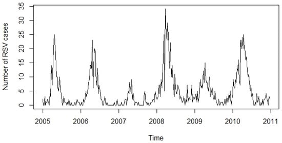
Figure 1.
The data set to be analyzed is the number of weekly cases of RSV reported from 1 January 2005 to 31 December 2010. In total, there are weekly observations.
3.2. Construction of the Artificial Neural Networks Models
We would now like to describe the general approach used in this work to determine the fitted ANN model. Initially, the data set n (n = 312 weeks) is divided into three: training set (), validation () and test (), such that: .
- Step 1.
- Determination of the structure of the network: We consider a MLP model, where q past lagged observations are used as input. The architecture of the model when there are hidden layers is depicted in Figure 2, and its associated mathematical representation is given as follows:where is the transfer function of the ith hidden layer, . In both cases, the sigmoid function is considered. The iterated method using a one-step model to generate forecasts iteratively is used.
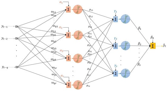 Figure 2. The architecture of the ANN considered.We choose the architecture of the neural network in two stages:
- Choice of number of hidden layers and neurons in the hidden layers: Assume that we have a large number of input variables , where is the maximum number of lags considered.
- (1)
- Estimate the model (5) with neurons in the hidden layer (), using the training dataset. Determine the predicted values and compute the Mean Square Error given by:
- (2)
- Increase one neuron in the hidden layer, i.e., take neurons, estimate the model and compute the
- (3)
- Test the new model:
- -
- If , then go to (2) (In case that always this condition is satisfied it could be possible to use as a stop criteria a maximum number of neurons and hidden layers). Once there are no improvements in the , proceed to increase the number of hidden layers and go to (2).
- -
- If , then we stop the process. Select an m as the number of neurons in the hidden layer and an s as the number of hidden layers.
- Choice of lags to be considered as input variables: Once the number of neurons in the hidden layer was defined, we proceeded to select the set of lags. To this end, the Influence Measure was calculated using the General (GIM) of the weights associated with each lag.The following backward sequential process based on MSE is applied: Given the maximum number of lags considered as input variables, and consider the network structure found previously.
- (i)
- Determine the individual significance of each of the lags, in the following way:
- (a)
- Determine the partial influence () of the i-th lag in the j-th neuron of the hidden layer:
- (b)
- Compute the general influence for the lag,
- (ii)
- Organize the lags in terms of their importance with regard to the forecast of the output variable using the GIM.
- (iii)
- Perform the backward selection process:
- (a)
- Estimate the network (5) with all the input lags. Compute the , and assume that this is the best value denoted by .
- (b)
- Then adjust th model removing the lag with lower , and compute the respective . Compare this value with the previous one: if , then stop the process and assume as the input variablesthe lags associated to the value of q that produced . Else go to (iii.c).
- (c)
- Update . For the new best model compute the of each of the input lags and go to step (iii.b).
- Step 2.
- Estimation of the model’s parameters: Once the number of hidden layers and the neurons in the hidden layers, as well as the set of delays that will be the input variables of the model, were determined, we proceeded to estimate the vector of parameters using the training data.The nonlinear least squares estimator of the , denoted by , is obtained using optimization algorithms based on gradients [66,67]. The estimator has the properties of an estimate of non-linear least squares [68]:
- (i)
- converges to when n increases.
- (ii)
- converges asymptotically to a multivariate normal distribution with vector of zero means and a covariance matrix that can be estimated consistently.
- Step 3.
- Selection of the best model: The scheme proposed by Zemouri et al. [44] is used. This is carried out times, so that in the end M models are estimated (from different starting points).Once the best model (5) has been selected, the iterated method is used to forecast, using a general one-step model to generate forecasts iteratively. To forecast one step ahead, all available historical observations are used. To forecast two steps ahead, the one-step forecast with historical data are used as inputs. The process continues until all the required forecasts are calculated.
4. Forecasting Results and Simulations
In this section, we present the numerical results and simulations of the artificial neural network models applied to the time series of the number of positive cases (by week) of RSV in Bogotá D.C., Colombia from 2005 to 2010. In addition, we compared our approach with a classical statistical technique of time series, such as SARIMA model. A seasonal plot of RSV cases reported weekly in each year is shown in Figure 3.
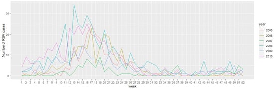
Figure 3.
Seasonal plot showing seasonal patterns for number of weekly cases of RSV reported.
From Figure 3, we can conclude that the weekly number of cases of RSV reported do not show a long-term growth or decrement pattern, but a seasonal variation; that is, similar patterns of behavior of the time series are observed at certain times of the year. In particular, the month of April is characterized by the highest number of cases reported, and the months with the lowest cases reported are September and October. This seasonal pattern has been studied in other articles using mechanistic models based on ordinary differential equations [7,11,12,15,24,69]. These previous approaches generate usually a smooth curve that represents the number of positive cases of RSV. For general behavior these mathematical models work relatively well, but are less accurate than empirical models such as the ones based on artificial neural networks. In addition, when the data of RSV-positive cases are irregular, stochastic models have been used to replicate the irregularity of the real world data [16,70]. However, these models are not particularly accurate, but give a good general behavior of the dynamics of RSV. We will see here that the artificial neural network models provide accurate estimates for short time forecasting and this is very useful for health authorities.
4.1. Experimental Conditions Used
In order to evaluate the forecasting capacity of an MLP model, under the proposed modeling approach, we consider a cross-validation procedure with different percentages of data for training, validation and testing of the networks: y For the selection of the structure of the network, a maximum of lags were considered.
To determine the network structure, we consider a maximum of lags as input variables, ten hidden layers and twenty five nodes in the hidden layers. For each training, we use a uniform distribution in the range of to generate the initial values of the weights and biases of the network. The back-propagation optimization algorithm is considered in this study. The different configurations that arise under these conditions are explored in accordance with the methodology described in Section 3, and using HO from R library. Other parameters considered are:
- Number of iterations in the learning over the training of the network: .
- Tolerance value for which the model should improve before the raining stops: stopping tolerance .
- Value to stop the training of the model when the metric does not improve for the value specified for the epochs of training: .
- We use the search strategy, the exploration of Lasso () and Ridge () regularization types varying their values on the interval . This with the aim of avoiding overfitting, reduce the variance and attenuate the effect of the correlation among the predictors.
- Setting the proportion of abandonment of the input layer to imporve the generalization:
As we have mentioned previously, we need to evaluate the performance of the adjusted MLP models using some metrics. After applying the approach explained in the previous section to obtain the structure of the artificial neural network and the estimation of the parameter vector , we found that to adequately predict the number of RSV cases, only one hidden layer is needed. In fact, there is a theorem that guarantees that one hidden layer is enough for many problems under certain conditions, and this has been used in previous works [59,60,71,72,73]. In addition, this result is in agreement with the literature related to ANNs for the prediction of time series. Zhang [74] showed that while there is flexibility in choosing the number of hidden layers and the number of hidden nodes in each layer, most network applications for forecasting purposes require only one hidden layer and a small number of hidden nodes. Additionally, there is evidence that the performance of neural networks to forecast time series is not very sensitive to the number of hidden nodes [75,76]. Moreover, empirical results suggest that the input layer (i.e., the number of previous lagged observations) is more important than the hidden layer in order to design an efficient ANN to forecast univariate time series [76,77,78].
In Table 1, the first column contains the percentage of cross-validation used to train the network, the second contains the number of neurons in the hidden layer, the third corresponds to the selected lag, then the four network performance measures are shown, and the last two columns contain the values of the measures and based on the test data set. From Table 1, we can conclude that the performance measures of the network using the validation data are better as the percentage of training considered increases. However, in the measurements obtained for the test data set, no pattern is observed related to the percentage of training used. In addition, we can see that the greater accuracy of the forecast (i.e., the higher value of ) is obtained with the maximum training percentage considered and two neurons in the hidden layer.

Table 1.
Comparison of performance measures of ANN models.
It is important to mention that the choice of the best configuration of the network should be made considering not only the and measures in the test set, but also the network performance measures. According to the results of Table 1, the best MLP network has the following characteristics: (i) the network that was trained and validated with 90% of the data and the remaining 10% was used as test data, (ii) the network has two neurons in the hidden layer and (iii) the input variables are the lagged observations. Thus, we select as the best model the MLP network with two neurons in the hidden layer, and taking the information from the previous weeks. The performance measures obtained by this MLP model guarantee its replicability and the accuracy of its forecasts, which is ideal for use in decision making [26,29,53,79].
In Figure 4, it is observed that only two peaks go outside the limits; that is, no more than 5% of the peaks are outside of these limits, and thus the series of residuals is likely to be white noise, which can be verified by the Augmented Dickey–Fuller Test (p-value = 0.01). Additionally, the absence of serial autocorrelation in the residuals is verified with the Ljung-Box test (p-value = 0.04133). Additionally, in Figure 5 it is observed that the residuals of the selected MLP model have an approximately Normal distribution.
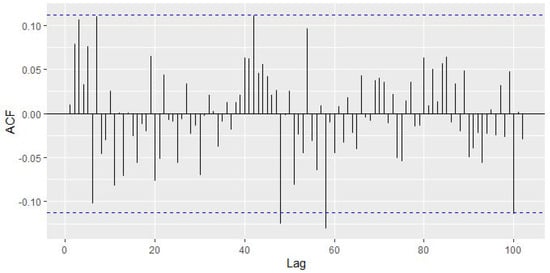
Figure 4.
Sample autocorrelation function of residuals of the selected MLP model.
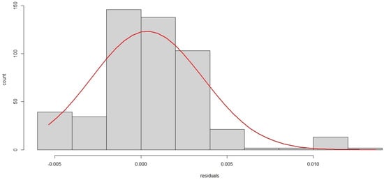
Figure 5.
Histogram of residuals of the selected MLP model.
Regarding the considered forecast horizons, note that they vary according to the amount of test data. In this case . From the results obtained, it can be deduced that the adjusted MLP model is capable of adequately forecasting the number of RSV cases corresponding to 32 weeks. The values forecasted by the selected MLP model are very close to the real values of the test set, as it can be observed in Figure 6. In this last Figure 6, note that the accuracy of forecast is given in all the data sets considered.
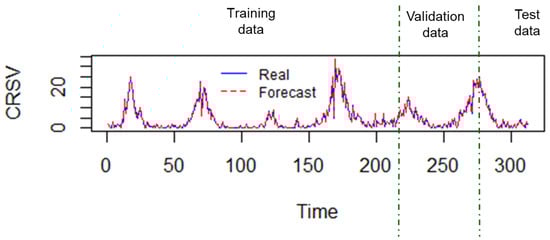
Figure 6.
Comparison of real values vs.the forecast values, in the 218 observations of training, the 62 of validation and the 32 of test.
4.2. Comparison of Artificial Neural Network with Traditional SARIMA Model
From the analysis of the RSV case series, it is found that it is a stationary series with a seasonal pattern. Stationarity is identified by the Augmented Dickey–Fuller test, which has a p-value = 0.01. Furthermore, from Figure 3, it is determined that the seasonal pattern is weeks. These characteristics make that from the traditional approach, the ideal candidate to forecast the series of cases of RSV is the SARIMA model. This means that in addition to our previous results using the ANN models, we would like to include the forecast using traditional SARIMA model in order to compare the performance of both approaches. In order to find an appropriate SARIMA model, we consider weeks examined per year and choose the values of and Q using the auto function in R [65].
Note that for the SARIMA model, it is not possible to apply the whole scheme proposed by Zemouri et al. [44] because in all M replicates, the same configuration of the model orders is always obtained. This implies that is assumed, and based on the estimated orders, and metrics are calculated using the test data. In Table 2, the first column contains the percentage of cross-validation used to fit of SARIMA model, the second corresponds to selected order, the third contains the ACCc obtained on the training data and the last two columns contain the values of measures and based on the test data set.
Table 2.
Comparison of performance measures of SARIMA models.
The selected SARIMA model was the model, corresponding to the cross-validation percentages . Forecasts from this model for the next ninety-four weeks are shown in Figure 7, where it is observed that the result provided by the traditional SARIMA model does not have a good forecasting capacity.
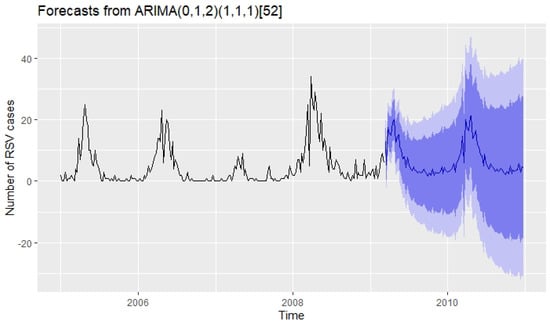
Figure 7.
In this case 218 weeks data were used to train the model. The measurements obtained with the 94 weeks test data were: and .
By performing goodness-of-fit tests with the model residuals, this is verified. The residuals from this model are shown in Figure 8. It is observed that although no more than of the peaks are outside the limits of the ACF, the Ljung-Box test (p-value = 0.8813) is not satisfied by the residuals of the model. Thus, the prediction intervals may not be accurate due to the correlated residuals [63].
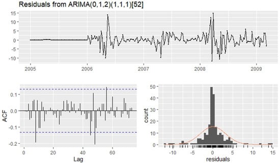
Figure 8.
Residuals from the model applied to the number of weekly RSV cases.
5. Discussion
In this paper, results obtained from the ANNs and SARIMA models were used for forecasting the number of confirmed positive cases of RSV for Bogotá D.C., Colombia. We varied the structures of the ANNs and SARIMA models. In addition, we use a variety of combinations for the training, validation and test datasets. We evaluated the accuracy of the different models using a variety of forecast performance metrics and based on these we make recommendations about the suitable models to forecast RSV cases. There are many metrics that have been used to evaluate prediction models such as RMSE, MAE, RRMSE [26]. Both ANN and SARIMA models show accurate results in forecasting for the data used in this study, but ANN has better forecasting accuracy. The advantage of the ANN over SARIMA is that it incorporates nonlinearity. The best ANN found in this research relies on using one hidden layer and just one neuron. Moreover, the fact of considering only the lagged observations as the input variables both in the network and in the SARIMA, tries to balance the complexity of the two models a bit. The results presented here in some way show the versatility of ANN to adjust its complexity depending on the type of application. Thus, this application to forecasting RSV cases is valuable for health authorities not only for RSV but for other diseases.
There are several approaches to carrying out epidemic forecasting. In particular, ANNs have been used previously to forecast some epidemics [26,28,29]. Epidemic forecasting is an important topic since it allows to design optimal prevention and control measures against infectious diseases. The selection of the forecasting approach or method is critical to improve the accuracy of epidemic forecast. Thus, studying different approaches for forecasting RSV is worth it. ANNs have been used to estimate the transmission rate for susceptible-infected-recovered (SIR) epidemic model. In addition, combination of different techniques with ANNs have been developed to deal with limited datasets [26]. In our work, we have enough data related to six years (2005–2011).
Based on the results of this research for RSV, we found that using 70% of the historical data for training and 20% for validation was the optimal combination. To train the selected MLP model, we used a variety of percentages of the historical data of RSV-positive cases. The best percentages were above . The optimal combination of percentages could change for historical data related to other diseases or even for RSV data for other regions or years. Therefore, we need to be careful for each particular disease. Although, this research related to positive cases of RSV for Bogotá D.C., Colombia provides insight and guidelines to forecast cases of RSV and other diseases that have a seasonal type behavior. Thus, the results obtained here can be also used or tested for other cities of Colombia and South-America.
In this work, we also applied the classical models. model, which does not have a good forecasting capacity of the RSV-positive reported cases as the best ANN model. In our study, we deal with seasonal behavior which makes the ANN model more suitable. This is because it is possible that the presence of seasonality in a time series leads to undesirable non-linear properties [80]. In [81], authors used a hybrid model combining the seasonal auto-regressive integrated moving average (ARIMA) model and nonlinear auto-regressive neural network (NARNN) to predict the expected incidence cases of hand-foot-mouth disease. They found that the found that the best-fitted hybrid model involved combining seasonal ARIMA and NARNN with 15 hidden units and 5 delays. In another work the authors used ARIMA and SARIMA time-series models to forecast the epidemiological trends of the COVID-19 pandemic [82]. The best model parameters of ARIMA and SARIMA for each country were selected manually, and then the model was used to forecast COVID-19 cases.
The proposed approach used here does not require standardization of the data, and is easy to implement, which allows its use for decision making in real time, which is very convenient for health institutions. We have seen all the health management issues that the COVID-19 pandemic has caused around the world related to the forecasting of hospitalizations due to the SARS-CoV-2. However, the COVID-19 pandemic is a more complex situation to forecast due to the change in the social behavior of the people.
6. Conclusions
In this paper, we constructed and developed different MLP models that appropriately describe the number of cases of RSV. The proposed model presents better results than the classical statistical technique of the time-series model. The adjusted MLP network is characterized by having a fairly high accuracy of forecasts of RSV-positive cases for Bogotá D.C., Colombia.
In summary, with the proposed methodology, here we can forecast with high accuracy the number of RSV-positive cases that will be reported in the next weeks. This can help health authorities from Colombia to make critical decisions in carrying out epidemic forecasts using the optimal ANN. In general, the outcomes of this research can lead health authorities to make the most convenient decisions regarding the slowing down of the RSV transmission in the human population, and the planning of medical resources to attend the children infected with RSV. In fact, similar studies have been presented recently which forecast infection and hospitalization related to SARS-CoV-2 [40,43,50,83,84]. Future directions of research include the introduction of weather variables in order to take into account climate variability over the years. Further studies can explore other exogenous factors that might affect the RSV epidemic in Colombia and other countries.
Author Contributions
Conceptualization, M.R.C. and G.G.-P.; Formal analysis, M.R.C., G.G.-P. and A.J.A.; Investigation, M.R.C., G.G.-P. and A.J.A.; Methodology, M.R.C., G.G.-P., and A.J.A.; Software, M.R.C., G.G.-P.; Supervision, G.G.-P., M.R.C. and A.J.A.; Validation, M.R.C., G.G.-P. and A.J.A.; Visualization, M.R.C., G.G.-P. and A.J.A.; Writing—original draft, G.G.-P., M.R.C. and A.J.A.; Writing—review and editing, G.G.-P., M.R.C. and A.J.A. All authors have read and agreed to the published version of the manuscript.
Funding
This research was funded by the University of Córdoba, Colombia, via FCB-06-19. The APC was funded by University of Córdoba, Colombia, via FCB-06-19.
Institutional Review Board Statement
Not applicable.
Acknowledgments
Funding support from the University of Córdoba, Colombia, via FCB-06-19 is gratefully acknowledged by the authors. The authors are grateful to the reviewers for their careful reading of this manuscript and their useful comments to improve the content of this paper.
Conflicts of Interest
The authors declare no conflict of interest.
Appendix A
The whole artificial neural network has input and output terminals. The processing units take an input and generate an output by means of mathematical expressions. Then, the output multiplied by a weight (of the link) becomes the input for another processing unit. At the end the output of the whole network is a combination of the inputs modified using complex relationships by several processing units. One additional aspect of the network is that it has a real-valued bias associated with each node, which allows the network to adapt to differences among the elements of the data set. It is important to remark that the whole artificial neural network has a parallel and distributed processing structure which allows faster computation in some cases [26,36,53,55,56]. The knowledge of the artificial neural network is acquired via a learning process through several input-output vectors and stored in inter-neuron connection strengths known as synaptic weights and bias (threshold) values. In Figure A1, it can be seen how one neuron can process several inputs with different weights to produce one output by means of the activation function and a bias.

Figure A1.
A neuron processing several inputs with different weights to produce one output by means of the activation function and a bias.
The simplest artificial neural network is composed of only of three layers. The first layer is the one which receives the input. The second layer is called the hidden layer, since it does not have a direct relationship with the inputs or outputs [36,73]. The last layer is the output, and this produces the output (prediction) of the whole artificial neural network. For more complex networks it is possible to have multiple hidden layers. Different layers might apply different transformations on their inputs. In fact, in the mathematical theory of artificial neural networks, universal approximation theorem type results state that a feed-forward network constructed of artificial neurons can approximate arbitrarily well real-valued continuous functions on compact subsets of [73,85]. However, this does not state how to find the artificial neural network.
We can summarize the overall artificial neural network process in the following way. The input is received by the input layer and after some mathematical transformation is passed to the following layer for another transformation. This transformation includes a multiplication by some weight w, and transfer and activation functions [26,36,53,55,56]. The activation function is a function that is Lipschitz continuous and monotonic [61]. The particular structure of the artificial neural network is highly variable. For instance, we can vary the number of layers, nodes in each layer, and/or transfer functions.
There are different types of artificial neural networks. The most well-known is the feedforward. In this neural network the information flows only from the input layer directly through the hidden layers to the output layer without loops. In addition, the feedforward networks can be built with different types of units. In most epidemic forecasts, neural network structures are in the form of a multilayer perceptron feed-forward fully connected network architecture [26]. The multilayer perceptron (MLP) neural network is the most popular network architecture and constitutes a non-linear function of its inputs, and is represented as a set of connected neurons. Since it is a feedforward network the information flows only in the forward direction, from the inputs to the outputs. Usually it has three layers (input, hidden and output), and uses sigmoid functions as transfer functions in the hidden layer. The functions of the output layer can be linear or sigmoidal depending on the problem [26,53,55,56]. In turn, an MLP with L hidden layers is defined as a function , given by
where is the response variable or output of the artificial neural network,
represents the input dimension, the output dimension, are the hidden dimensions, is an Euclidean vector space, and ∘ denotes the composition operator,
where g is an activation function, for any is an affine mapping defined by for some weight matriz and bias vector , and is the output layer [61]. In this setting, the MLP’s parameters are given by
In Figure A2, the topology of a multilayer perceptron neural network with two hidden layers can be seen: the first hidden layer has q neurons, and the second r neurons. Each input is connected to each neuron in the first hidden layer; the output of each neuron in the first layer is connected to each neuron in the second layer and so on. The strengths of these connections are called synaptic weights: and In addition, the neurons of each hidden layer have a bias: , which can take the same value in the hidden layer.

Figure A2.
Topology of a multilayer perceptron neural network with two hidden layers: the first hidden layer has q neurons, and the second r neurons. Each input is connected to each neuron in the first hidden layer, the output of each neuron in the first layer is connected to each neuron in the second layer and so on. The strengths of these connections are called synaptic weights: and . In addition, the neurons of each hidden layer have a bias: , which can take the same value in the hidden layer.
References
- Morris, J.; Blount, R., Jr.; Savage, R. Recovery of cytopathogenic agent from chimpanzees with goryza. Proc. Soc. Exp. Biol. Med. 1956, 92, 544–549. [Google Scholar] [CrossRef] [PubMed]
- Hall, C.B. Respiratory syncytial virus and parainfluenza virus. N. Engl. J. Med. 2001, 344, 1917–1928. [Google Scholar] [CrossRef]
- Chanock, R.M.; Parrott, R.H.; Cook, K.; Andrews, B.; Bell, J.; Reichelderfer, T.; Kapikian, A.Z.; Mastrota, F.; Huebner, R.J. Newly recognized myxoviruses from children with respiratory disease. N. Engl. J. Med. 1958, 258, 207–213. [Google Scholar] [CrossRef]
- Gwatkin, D.R. How many die? A set of demographic estimates of the annual number of infant and child deaths in the world. Am. J. Public Health 1980, 70, 1286–1289. [Google Scholar] [CrossRef]
- Aranda-Lozano, D.F.; González-Parra, G.C.; Querales, J. Modelling respiratory syncytial virus (RSV) transmission children aged less than five years-old. Rev. Salud Pública 2013, 15, 689–700. [Google Scholar] [PubMed]
- Shi, T.; McAllister, D.A.; O’Brien, K.L.; Simoes, E.A.; Madhi, S.A.; Gessner, B.D.; Polack, F.P.; Balsells, E.; Acacio, S.; Aguayo, C.; et al. Global, regional, and national disease burden estimates of acute lower respiratory infections due to respiratory syncytial virus in young children in 2015: A systematic review and modelling study. Lancet 2017, 390, 946–958. [Google Scholar] [CrossRef]
- Arenas, A.; González, G.; Jódar, L. Existence of periodic solutions in a model of respiratory syncytial virus RSV. J. Math. Anal. Appl. 2008, 344, 969–980. [Google Scholar] [CrossRef][Green Version]
- González-Parra, G.; Dobrovolny, H.M. Assessing uncertainty in A2 respiratory syncytial virus viral dynamics. Comput. Math. Methods Med. 2015, 2015. [Google Scholar] [CrossRef][Green Version]
- González-Parra, G.; Dobrovolny, H.M. The rate of viral transfer between upper and lower respiratory tracts determines RSV illness duration. J. Math. Biol. 2019, 79, 467–483. [Google Scholar] [CrossRef] [PubMed]
- Thongpan, I.; Vongpunsawad, S.; Poovorawan, Y. Respiratory syncytial virus infection trend is associated with meteorological factors. Sci. Rep. 2020, 10, 1–7. [Google Scholar] [CrossRef]
- Weber, A.; Weber, M.; Milligan, P. Modeling epidemics caused by respiratory syncytial virus (RSV). Math. Biosci. 2001, 172, 95–113. [Google Scholar] [CrossRef]
- White, L.; Mandl, J.; Gomes, M.; Bodley-Tickell, A.; Cane, P.; Perez-Brena, P.; Aguilar, J.; Siqueira, M.; Portes, S.; Straliotto, S.; et al. Understanding the transmission dynamics of respiratory syncytial virus using multiple time-series and nested models. Math. Biosci. 2007, 209, 222–239. [Google Scholar] [CrossRef]
- Hethcote, H.W. Mathematics of infectious diseases. SIAM Rev. 2005, 42, 599–653. [Google Scholar] [CrossRef]
- Castillo-Chavez, C.; Brauer, F. Mathematical Models in Population Biology and Epidemiology; Springer: New York, NY, USA, 2012. [Google Scholar]
- Hogan, A.B.; Glass, K.; Moore, H.C.; Anderssen, R.S. Age structures in mathematical models for infectious diseases, with a case study of respiratory syncytial virus. In Applications + Practical Conceptualization + Mathematics = Fruitful Innovation; Springer: Berlin/Heidelberg, Germany, 2016; pp. 105–116. [Google Scholar]
- Arenas, A.J.; González-Parra, G.; Moraño, J.A. Stochastic modeling of the transmission of respiratory syncytial virus (RSV) in the region of Valencia, Spain. Biosystems 2009, 96, 206–212. [Google Scholar] [CrossRef]
- Keeling, M.J.; Eames, K.T. Networks and epidemic models. J. R. Soc. Interface 2005, 2, 295–307. [Google Scholar] [CrossRef] [PubMed]
- Acedo, L.; Burgos, C.; Hidalgo, J.I.; Sánchez-Alonso, V.; Villanueva, R.J.; Villanueva-Oller, J. Calibrating a large network model describing the transmission dynamics of the human papillomavirus using a particle swarm optimization algorithm in a distributed computing environment. Int. J. High Perform. Comput. Appl. 2018, 32, 721–728. [Google Scholar] [CrossRef]
- Malik, H.A.M.; Mahesar, A.W.; Abid, F.; Waqas, A.; Wahiddin, M.R. Two-mode network modeling and analysis of dengue epidemic behavior in Gombak, Malaysia. Appl. Math. Model. 2017, 43, 207–220. [Google Scholar] [CrossRef]
- González-Parra, G.; Villanueva, R.J.; Ruiz-Baragaño, J.; Moraño, J.A. Modelling influenza A (H1N1) 2009 epidemics using a random network in a distributed computing environment. Acta Trop. 2015, 143, 29–35. [Google Scholar] [CrossRef] [PubMed]
- Della Rossa, F.; Salzano, D.; Di Meglio, A.; De Lellis, F.; Coraggio, M.; Calabrese, C.; Guarino, A.; Cardona-Rivera, R.; De Lellis, P.; Liuzza, D.; et al. A network model of Italy shows that intermittent regional strategies can alleviate the COVID-19 epidemic. Nat. Commun. 2020, 11, 1–9. [Google Scholar] [CrossRef]
- Jahn, B.; Sroczynski, G.; Bicher, M.; Rippinger, C.; Mühlberger, N.; Santamaria, J.; Urach, C.; Schomaker, M.; Stojkov, I.; Schmid, D.; et al. Targeted COVID-19 Vaccination (TAV-COVID) Considering Limited Vaccination Capacities—An Agent-Based Modeling Evaluation. Vaccines 2021, 9, 434. [Google Scholar] [CrossRef] [PubMed]
- Bonate, P.L. Pharmacokinetic-Pharmacodynamic Modeling and Simulation; Springer: Berlin/Heidelberg, Germany, 2011; Volume 20. [Google Scholar]
- González-Parra, G.; Querales, J.F.; Aranda, D. Prediction of the respiratory syncitial virus epidemic using climate variables in Bogotá, DC. Biomédica 2016, 36, 378–389. [Google Scholar] [CrossRef]
- Núñez, L.M.; Aranda, D.F.; Jaramillo, A.C.; Moyano, L.F.; Osorio, E.d.J. Chronology of a pandemic: The new influenza A (H1N1) in Bogota, 2009–2010. Rev. Salud Pública 2011, 13, 480–491. [Google Scholar]
- Philemon, M.D.; Ismail, Z.; Dare, J. A review of epidemic forecasting using artificial neural networks. Int. J. Epidemiol. Res. 2019, 6, 132–143. [Google Scholar]
- Bharambe, A.A.; Kalbande, D.R. Techniques and approaches for disease outbreak prediction: A survey. In Proceedings of the ACM Symposium on Women in Research 2016, Indore, India, 21–22 March 2016; pp. 100–102. [Google Scholar]
- Saberian, F.; Zamani, A.; Gooya, M.M.; Hemmati, P.; Shoorehdeli, M.A.; Teshnehlab, M. Prediction of seasonal influenza epidemics in Tehran using artificial neural networks. In Proceedings of the 2014 22nd Iranian Conference on Electrical Engineering (ICEE), Tehran, Iran, 20–22 May 2014; pp. 1921–1923. [Google Scholar]
- Zhang, G.; Patuwo, B.E.; Hu, M.Y. Forecasting with artificial neural networks: The state of the art. Int. J. Forecast. 1998, 14, 35–62. [Google Scholar] [CrossRef]
- Chen, Z.; Zhu, Y.; Wang, Y.; Zhou, W.; Yan, Y.; Zhu, C.; Zhang, X.; Sun, H.; Ji, W. Association of meteorological factors with childhood viral acute respiratory infections in subtropical China: An analysis over 11 years. Arch. Virol. 2014, 159, 631–639. [Google Scholar] [CrossRef] [PubMed]
- Li, Y.; Reeves, R.M.; Wang, X.; Bassat, Q.; Brooks, W.A.; Cohen, C.; Moore, D.P.; Nunes, M.; Rath, B.; Campbell, H.; et al. Global patterns in monthly activity of influenza virus, respiratory syncytial virus, parainfluenza virus, and metapneumovirus: A systematic analysis. Lancet Glob. Health 2019, 7, e1031–e1045. [Google Scholar] [CrossRef]
- Chae, Y.T.; Horesh, R.; Hwang, Y.; Lee, Y.M. Artificial neural network model for forecasting sub-hourly electricity usage in commercial buildings. Energy Build. 2016, 111, 184–194. [Google Scholar] [CrossRef]
- Ghiassi, M.; Saidane, H.; Zimbra, D. A dynamic artificial neural network model for forecasting time-series events. Int. J. Forecast. 2005, 21, 341–362. [Google Scholar] [CrossRef]
- Qiu, M.; Song, Y. Predicting the direction of stock market index movement using an optimized artificial neural network model. PLoS ONE 2016, 11, e0155133. [Google Scholar] [CrossRef] [PubMed]
- Liyanaarachchi, V.C.; Nishshanka, G.K.S.H.; Nimarshana, P.H.V.; Ariyadasa, T.U.; Attalage, R.A. Development of an artificial neural network model to simulate the growth of microalga Chlorella vulgaris incorporating the effect of micronutrients. J. Biotechnol. 2020, 312, 44–55. [Google Scholar] [CrossRef]
- Tino, P.; Benuskova, L.; Sperduti, A. Artificial neural network models. In Springer Handbook of Computational Intelligence; Springer: Berlin/Heidelberg, Germany, 2015; pp. 455–471. [Google Scholar]
- Hong, Y.; Hou, B.; Jiang, H.; Zhang, J. Machine learning and artificial neural network accelerated computational discoveries in materials science. Wiley Interdiscip. Rev. Comput. Mol. Sci. 2020, 10, e1450. [Google Scholar] [CrossRef]
- Walczak, S. Artificial neural networks. In Advanced Methodologies and Technologies in Artificial Intelligence, Computer Simulation, and Human-Computer Interaction; IGI Global: Hershey, PA, USA, 2019; pp. 40–53. [Google Scholar]
- Zou, J.; Han, Y.; So, S.S. Overview of artificial neural networks. Artif. Neural Netw. 2008, 458, 14–22. [Google Scholar]
- Rasjid, Z.E.; Setiawan, R.; Effendi, A. A Comparison: Prediction of Death and Infected COVID-19 Cases in Indonesia Using Time Series Smoothing and LSTM Neural Network. Procedia Comput. Sci. 2021, 179, 982–988. [Google Scholar] [CrossRef]
- Lindemann, B.; Müller, T.; Vietz, H.; Jazdi, N.; Weyrich, M. A survey on long short-term memory networks for time series prediction. Procedia CIRP 2021, 99, 650–655. [Google Scholar] [CrossRef]
- Yadav, A.; Jha, C.; Sharan, A. Optimizing LSTM for time series prediction in Indian stock market. Procedia Comput. Sci. 2020, 167, 2091–2100. [Google Scholar] [CrossRef]
- Moftakhar, L.; Mozhgan, S.; Safe, M.S. Exponentially increasing trend of infected patients with COVID-19 in Iran: A comparison of neural network and ARIMA forecasting models. Iran. J. Public Health 2020, 49, 92–100. [Google Scholar] [CrossRef]
- Zemouri, R.; Gouriveau, R.; Zerhouni, N. Defining and applying prediction performance metrics on a recurrente NARX time series model. Neurocomputing 2010, 73, 2506–2521. [Google Scholar] [CrossRef]
- Barbosa, J.; Parra, B.; Alarcón, L.; Quiñones, F.I.; López, E.; Franco, M.A. Prevalence and periodicity of respiratory syncytial virus in Colombia. Rev. Acad. Colomb. Cienc. Exactas Físicas Nat. 2017, 41, 435–446. [Google Scholar] [CrossRef]
- Gamba-Sanchez, N.; Rodriguez-Martinez, C.; Sossa-Briceño, M. Epidemic activity of respiratory syncytial virus is related to temperature and rainfall in equatorial tropical countries. Epidemiol. Infect. 2016, 144, 2057–2063. [Google Scholar] [CrossRef] [PubMed]
- Casado-Vara, R.; Martin del Rey, A.; Pérez-Palau, D.; de-la Fuente-Valentín, L.; Corchado, J.M. Web Traffic Time Series Forecasting Using LSTM Neural Networks with Distributed Asynchronous Training. Mathematics 2021, 9, 421. [Google Scholar] [CrossRef]
- Cicek, Z.I.E.; Ozturk, Z.K. Optimizing the artificial neural network parameters using a biased random key genetic algorithm for time series forecasting. Appl. Soft Comput. 2021, 102, 107091. [Google Scholar] [CrossRef]
- Hewamalage, H.; Bergmeir, C.; Bandara, K. Recurrent neural networks for time series forecasting: Current status and future directions. Int. J. Forecast. 2021, 37, 388–427. [Google Scholar] [CrossRef]
- Katris, C. A time series-based statistical approach for outbreak spread forecasting: Application of COVID-19 in Greece. Expert Syst. Appl. 2021, 166, 114077. [Google Scholar] [CrossRef] [PubMed]
- Moghanlo, S.; Alavinejad, M.; Oskoei, V.; Saleh, H.N.; Mohammadi, A.A.; Mohammadi, H.; DerakhshanNejad, Z. Using artificial neural networks to model the impacts of climate change on dust phenomenon in the Zanjan region, north-west Iran. Urban Clim. 2021, 35, 100750. [Google Scholar] [CrossRef]
- Haykin, S. Neural Networks: A Comprehensive Foundation; Macmillan Publishing: New York, NY, USA, 1994. [Google Scholar]
- Haykin, S.; Network, N. A comprehensive foundation. Neural Netw. 2004, 2, 41. [Google Scholar]
- Hopfield, J.J. Artificial neural networks. IEEE Circuits Devices Mag. 1988, 4, 3–10. [Google Scholar] [CrossRef]
- Graupe, D. Principles of Artificial Neural Networks; World Scientific: Singapore, 2013; Volume 7. [Google Scholar]
- Mehrotra, K.; Mohan, C.K.; Ranka, S. Elements of Artificial Neural Networks; MIT Press: Cambridge, MA, USA, 1997. [Google Scholar]
- Hornik, K. Approximation capabilities of multilayer feedforward networks. Neural Netw. 1991, 4, 251–257. [Google Scholar] [CrossRef]
- Buehler, H.; Gonon, L.; Teichmann, J.; Wood, B. Deep Hedging. Quant. Financ. 2019, 19, 1271–1291. [Google Scholar] [CrossRef]
- Hornik, K.; Stinchcombe, M.; White, H. Multilayer feedforward networks are universal approximators. Neural Netw. 1989, 2, 359–366. [Google Scholar] [CrossRef]
- Hornik, K.; Stinchcombe, M.; White, H. Universal approximation of an unknown mapping and its derivatives using multilayer feedforward networks. Neural Netw. 1990, 3, 551–560. [Google Scholar] [CrossRef]
- Wiese, M.; Knobloch, R.; Korn, R.; Kretschmer, P. Quant GANs: Deep generation of financial time series. Quant. Financ. 2020, 20, 1419–1440. [Google Scholar] [CrossRef]
- Egrioglu, E.; Aladag, C.; Gunay, S. A new model selection strategy in artificial neural networks. Appl. Math. Comput. 2008, 195, 591–597. [Google Scholar]
- Hyndman, R.; Athanasopoulos, G. Forecasting: Principles and Practice, 3rd ed.; OTexts: Melbourne, Australia, 2021. [Google Scholar]
- Oliveira, P.J.; Steffen, J.; Cheung, P. Parameter estimation of seasonal ARIMA models for water demand forecasting using the Harmony Search Algorithm. Procedia Eng. 2017, 186, 177–185. [Google Scholar] [CrossRef]
- R Core Team. R: A Language and Environment for Statistical Computing; R Foundation for Statistical Computing: Vienna, Austria, 2020. [Google Scholar]
- May, R.; Dandy, G.; Maier, H. Review of Input Variable Selection Methods for Artificial Neural Networks. Neural Process. Lett. 2015, 41, 249–258. [Google Scholar]
- Igel, C.; Husken, M. Empirical evaluation of the improved Rprop learning algorithms. Neurocomputing 2003, 50, 105–123. [Google Scholar] [CrossRef]
- Franses, P.; Dijk, D. Non-Linear Time Series Models in Empirical Finance; Cambridge University Press: New York, NY, USA, 2000. [Google Scholar]
- White, L.; Waris, M.; Cane, P.; Nokes, D.; Medley, G. The transmission dynamics of groups A and B human respiratory syncytial virus (hRSV) in England and Wales and Finland: Seasonality and cross-protection. Epidemiol. Infect. 2005, 133, 279–289. [Google Scholar] [CrossRef]
- González-Parra, G.; Arenas, A.J.; Cogollo, M.R. Positivity and boundedness of solutions for a stochastic seasonal epidemiological model for respiratory syncytial virus (RSV). Ingeniería Cienc. 2017, 13, 95–121. [Google Scholar] [CrossRef]
- Chui, C.K.; Li, X. Approximation by ridge functions and neural networks with one hidden layer. J. Approx. Theory 1992, 70, 131–141. [Google Scholar] [CrossRef]
- Kurková, V. Kolmogorov’s theorem is relevant. Neural Comput. 1991, 3, 617–622. [Google Scholar] [CrossRef]
- Li, X. Simultaneous approximations of multivariate functions and their derivatives by neural networks with one hidden layer. Neurocomputing 1996, 12, 327–343. [Google Scholar] [CrossRef]
- Zhang, T.; Liu, J.; Teng, Z. Existence of positive periodic solutions of an SEIR model with periodic coefficients. Appl. Math. 2012, 57, 601–616. [Google Scholar] [CrossRef]
- Bakirtzis, A.; Petridis, V.; Kiartzis, S.; Alexiadis, M.; Maissis, A. A neural network short term load forecasting model for the Greek power system. IEEE Trans. Power Syst. 1996, 11, 858–863. [Google Scholar] [CrossRef]
- Zhang, G.P. An investigation of neural networks for linear time-series forecasting. Comput. Oper. Res. 2001, 28, 1183–1202. [Google Scholar] [CrossRef]
- Ghysels, M.M.; Terasvirta, T.; Rech, G. Building neural network models for time series: A statistical approach. J. Forecast. 2006, 25, 49–75. [Google Scholar]
- Lennox, B.; Montague, G.A.; Frith, A.M.; Gent, C.; Bevan, V. Industrial application of neural networks—An investigation. J. Process. Control 2001, 11, 497–507. [Google Scholar] [CrossRef]
- Chakraborty, T.; Chattopadhyay, S.; Ghosh, I. Forecasting dengue epidemics using a hybrid methodology. Phys. A Stat. Mech. Its Appl. 2019, 527, 121266. [Google Scholar] [CrossRef]
- Ghysels, E.; Granger, C.W.; Siklos, P.L. Is seasonal adjustment a linear or nonlinear data-filtering process? J. Bus. Econ. Stat. 1996, 14, 374–386. [Google Scholar]
- Yu, L.; Zhou, L.; Tan, L.; Jiang, H.; Wang, Y.; Wei, S.; Nie, S. Application of a new hybrid model with seasonal auto-regressive integrated moving average (ARIMA) and nonlinear auto-regressive neural network (NARNN) in forecasting incidence cases of HFMD in Shenzhen, China. PLoS ONE 2014, 9, e98241. [Google Scholar] [CrossRef]
- ArunKumar, K.; Kalaga, D.V.; Kumar, C.M.S.; Chilkoor, G.; Kawaji, M.; Brenza, T.M. Forecasting the dynamics of cumulative COVID-19 cases (confirmed, recovered and deaths) for top-16 countries using statistical machine learning models: Auto-Regressive Integrated Moving Average (ARIMA) and Seasonal Auto-Regressive Integrated Moving Average (SARIMA). Appl. Soft Comput. 2021, 103, 107161. [Google Scholar]
- Distante, C.; Pereira, I.G.; Goncalves, L.M.G.; Piscitelli, P.; Miani, A. Forecasting Covid-19 Outbreak Progression in Italian Regions: A model based on neural network training from Chinese data. medRxiv 2020. [Google Scholar] [CrossRef]
- Hawas, M. Generated time-series prediction data of COVID-19’s daily infections in Brazil by using recurrent neural networks. Data Brief 2020, 32, 106175. [Google Scholar] [CrossRef] [PubMed]
- Csáji, B.C. Approximation with artificial neural networks. Fac. Sci. Etvs Lornd Univ. Hung. 2001, 24, 7. [Google Scholar]
Publisher’s Note: MDPI stays neutral with regard to jurisdictional claims in published maps and institutional affiliations. |
© 2021 by the authors. Licensee MDPI, Basel, Switzerland. This article is an open access article distributed under the terms and conditions of the Creative Commons Attribution (CC BY) license (https://creativecommons.org/licenses/by/4.0/).