Modeling and Forecasting Cases of RSV Using Artificial Neural Networks
Abstract
1. Introduction
2. Preliminaries
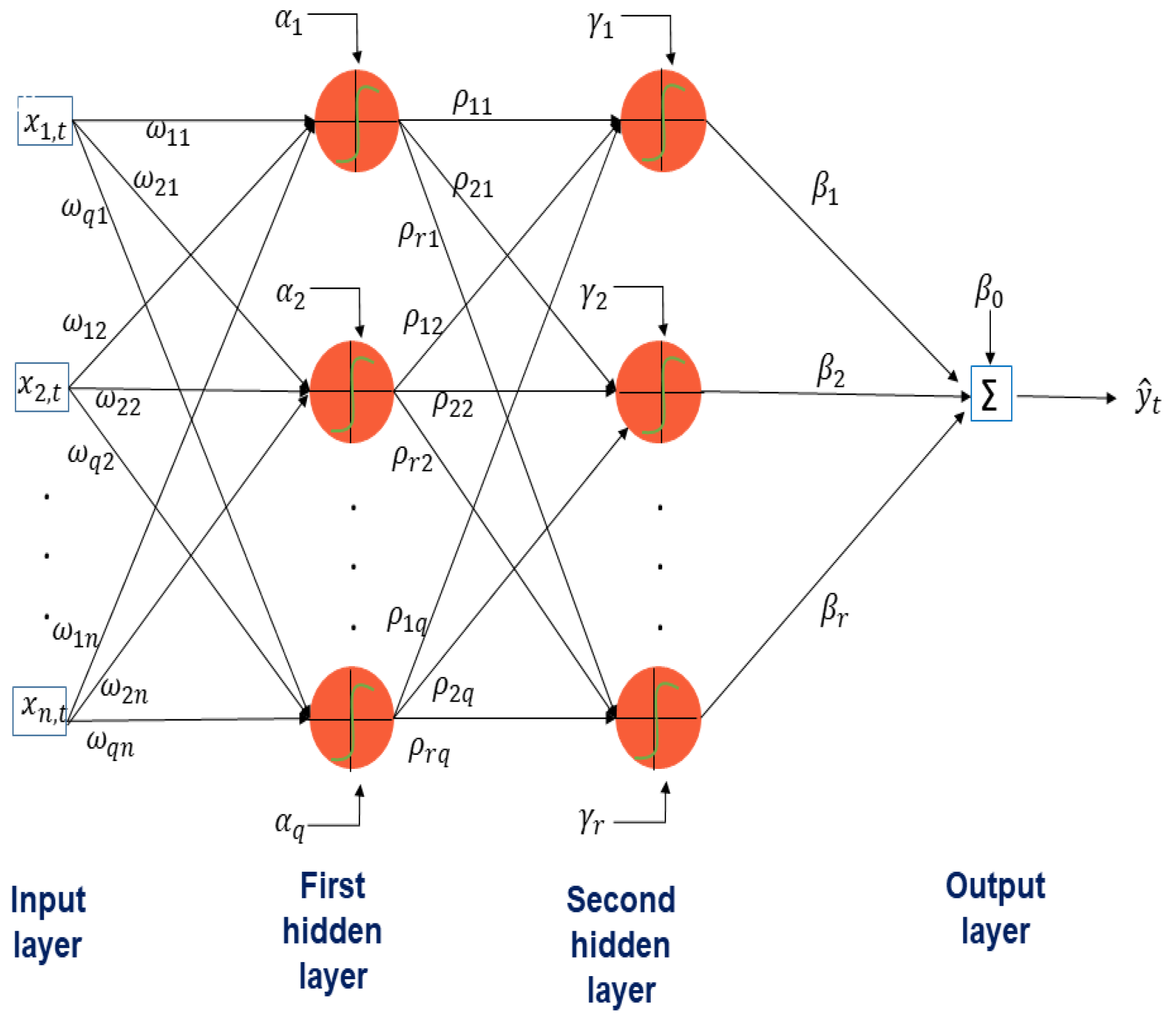
2.1. Artificial Neural Network
2.2. Cross-Validation Process in ANN Model Parameter Estimation
- Step 1.
- Perform from to M times, from different starting points:
- Train the network using the training data.
- Validate the trained network using the validation data. Calculate the mean forecast error and the forecast variance on the validation set as follows:
- Step 2.
- Calculate the following measures to evaluate the performance of network forecasts:
- Timeliness: is given by the global mean of all the M values of :The perfect score is . For a small value of the timeliness, the probability to have a prediction close to the real value can be significant.
- Precision: is given by the global mean of all the M values of :The perfect score is . For a small value of the precision, the probability to have predictions grouped together can be significant.
- Repeatability: is given by the standard deviation of both and :The perfect score is , it means that at each training/running time i, the neural model gives the same performances on the validation set.
- Accuracy: is given byIf the artificial neural network model has good timeliness, precision and is completely repeatable, and the prediction given by the model is very close to the real data, then a large value of the accuracy parameter gives great confidence in the prediction.
- Step 3.
- From M runs performed for the network, select the model with lowest and . Additionally, it must be verified that takes a large value and , and take small values over the validation set. In this way, overfitting and underfitting problems are avoided.
- Step 4.
- Finally, the choice of the best model is made by calculating the measures and with the data of the test set. The best model is the one with the smallest measures of and .
2.3. SARIMA Model
- is the study variable in time t;
- B is the backward shift (or lag) operator, such that ;
- is the seasonal Autoregressive (AR) operator of order P;
- is the regular AR operator of order p;
- is the seasonal differences and is the regular differences;
- is the seasonal moving average (MA) operator of order Q;
- is the regular MA operator of order q;
- is a white noise process.
3. Materials and Methods
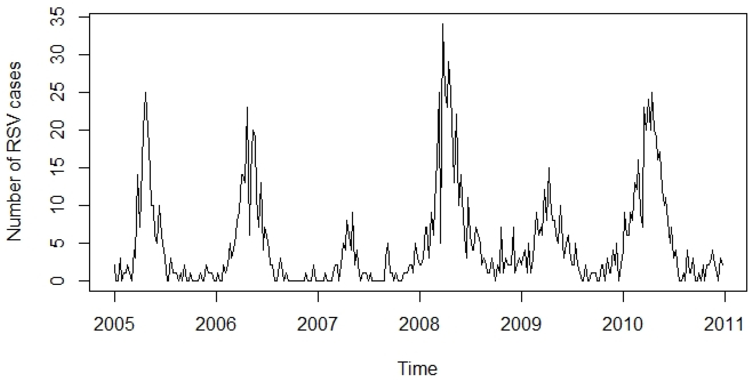
3.1. Data
3.2. Construction of the Artificial Neural Networks Models
- Step 1.
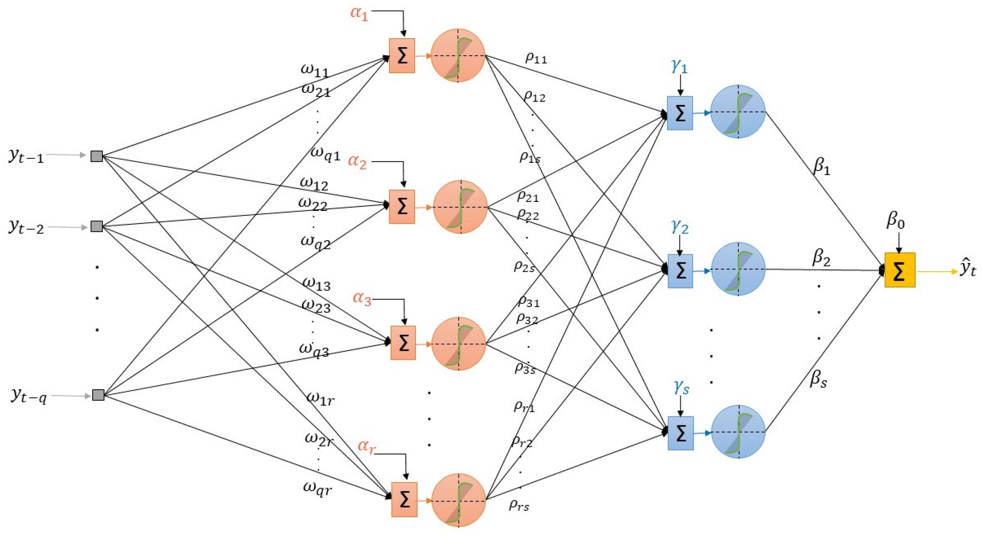
- Determination of the structure of the network: We consider a MLP model, where q past lagged observations are used as input. The architecture of the model when there are hidden layers is depicted in Figure 2, and its associated mathematical representation is given as follows:where is the transfer function of the ith hidden layer, . In both cases, the sigmoid function is considered. The iterated method using a one-step model to generate forecasts iteratively is used.We choose the architecture of the neural network in two stages:
- Choice of number of hidden layers and neurons in the hidden layers: Assume that we have a large number of input variables , where is the maximum number of lags considered.
- (1)
- Estimate the model (5) with neurons in the hidden layer (), using the training dataset. Determine the predicted values and compute the Mean Square Error given by:
- (2)
- Increase one neuron in the hidden layer, i.e., take neurons, estimate the model and compute the
- (3)
- Test the new model:
- -
- If , then go to (2) (In case that always this condition is satisfied it could be possible to use as a stop criteria a maximum number of neurons and hidden layers). Once there are no improvements in the , proceed to increase the number of hidden layers and go to (2).
- -
- If , then we stop the process. Select an m as the number of neurons in the hidden layer and an s as the number of hidden layers.
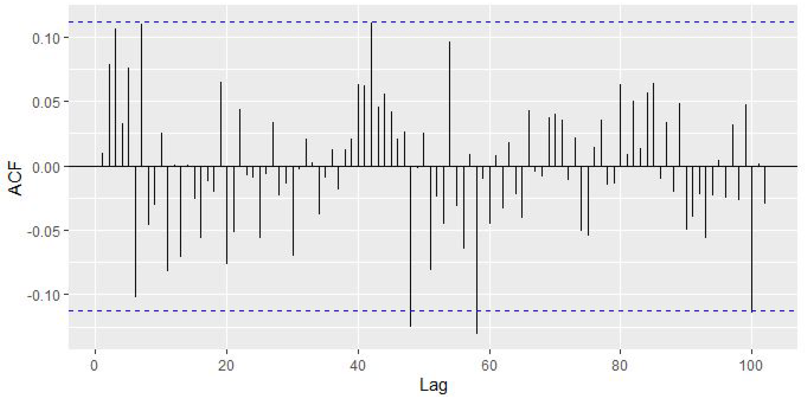
- Choice of lags to be considered as input variables: Once the number of neurons in the hidden layer was defined, we proceeded to select the set of lags. To this end, the Influence Measure was calculated using the General (GIM) of the weights associated with each lag.The following backward sequential process based on MSE is applied: Given the maximum number of lags considered as input variables, and consider the network structure found previously.
- (i)
- Determine the individual significance of each of the lags, in the following way:
- (a)
- Determine the partial influence () of the i-th lag in the j-th neuron of the hidden layer:
- (b)
- Compute the general influence for the lag,
- (ii)
- Organize the lags in terms of their importance with regard to the forecast of the output variable using the GIM.
- (iii)
- Perform the backward selection process:
- (a)
- Estimate the network (5) with all the input lags. Compute the , and assume that this is the best value denoted by .
- (b)
- Then adjust th model removing the lag with lower , and compute the respective . Compare this value with the previous one: if , then stop the process and assume as the input variablesthe lags associated to the value of q that produced . Else go to (iii.c).
- (c)
- Update . For the new best model compute the of each of the input lags and go to step (iii.b).
- Step 2.
- Estimation of the model’s parameters: Once the number of hidden layers and the neurons in the hidden layers, as well as the set of delays that will be the input variables of the model, were determined, we proceeded to estimate the vector of parameters using the training data.The nonlinear least squares estimator of the , denoted by , is obtained using optimization algorithms based on gradients [66,67]. The estimator has the properties of an estimate of non-linear least squares [68]:
- (i)
- converges to when n increases.
- (ii)
- converges asymptotically to a multivariate normal distribution with vector of zero means and a covariance matrix that can be estimated consistently.
- Step 3.
- Selection of the best model: The scheme proposed by Zemouri et al. [44] is used. This is carried out times, so that in the end M models are estimated (from different starting points).Once the best model (5) has been selected, the iterated method is used to forecast, using a general one-step model to generate forecasts iteratively. To forecast one step ahead, all available historical observations are used. To forecast two steps ahead, the one-step forecast with historical data are used as inputs. The process continues until all the required forecasts are calculated.
4. Forecasting Results and Simulations
4.1. Experimental Conditions Used
- Number of iterations in the learning over the training of the network: .
- Tolerance value for which the model should improve before the raining stops: stopping tolerance .
- Value to stop the training of the model when the metric does not improve for the value specified for the epochs of training: .
- We use the search strategy, the exploration of Lasso () and Ridge () regularization types varying their values on the interval . This with the aim of avoiding overfitting, reduce the variance and attenuate the effect of the correlation among the predictors.
- Setting the proportion of abandonment of the input layer to imporve the generalization:
4.2. Comparison of Artificial Neural Network with Traditional SARIMA Model
5. Discussion
6. Conclusions
Author Contributions
Funding
Institutional Review Board Statement
Acknowledgments
Conflicts of Interest
Appendix A

References
- Morris, J.; Blount, R., Jr.; Savage, R. Recovery of cytopathogenic agent from chimpanzees with goryza. Proc. Soc. Exp. Biol. Med. 1956, 92, 544–549. [Google Scholar] [CrossRef] [PubMed]
- Hall, C.B. Respiratory syncytial virus and parainfluenza virus. N. Engl. J. Med. 2001, 344, 1917–1928. [Google Scholar] [CrossRef]
- Chanock, R.M.; Parrott, R.H.; Cook, K.; Andrews, B.; Bell, J.; Reichelderfer, T.; Kapikian, A.Z.; Mastrota, F.; Huebner, R.J. Newly recognized myxoviruses from children with respiratory disease. N. Engl. J. Med. 1958, 258, 207–213. [Google Scholar] [CrossRef]
- Gwatkin, D.R. How many die? A set of demographic estimates of the annual number of infant and child deaths in the world. Am. J. Public Health 1980, 70, 1286–1289. [Google Scholar] [CrossRef]
- Aranda-Lozano, D.F.; González-Parra, G.C.; Querales, J. Modelling respiratory syncytial virus (RSV) transmission children aged less than five years-old. Rev. Salud Pública 2013, 15, 689–700. [Google Scholar] [PubMed]
- Shi, T.; McAllister, D.A.; O’Brien, K.L.; Simoes, E.A.; Madhi, S.A.; Gessner, B.D.; Polack, F.P.; Balsells, E.; Acacio, S.; Aguayo, C.; et al. Global, regional, and national disease burden estimates of acute lower respiratory infections due to respiratory syncytial virus in young children in 2015: A systematic review and modelling study. Lancet 2017, 390, 946–958. [Google Scholar] [CrossRef]
- Arenas, A.; González, G.; Jódar, L. Existence of periodic solutions in a model of respiratory syncytial virus RSV. J. Math. Anal. Appl. 2008, 344, 969–980. [Google Scholar] [CrossRef][Green Version]
- González-Parra, G.; Dobrovolny, H.M. Assessing uncertainty in A2 respiratory syncytial virus viral dynamics. Comput. Math. Methods Med. 2015, 2015. [Google Scholar] [CrossRef]
- González-Parra, G.; Dobrovolny, H.M. The rate of viral transfer between upper and lower respiratory tracts determines RSV illness duration. J. Math. Biol. 2019, 79, 467–483. [Google Scholar] [CrossRef] [PubMed]
- Thongpan, I.; Vongpunsawad, S.; Poovorawan, Y. Respiratory syncytial virus infection trend is associated with meteorological factors. Sci. Rep. 2020, 10, 1–7. [Google Scholar] [CrossRef]
- Weber, A.; Weber, M.; Milligan, P. Modeling epidemics caused by respiratory syncytial virus (RSV). Math. Biosci. 2001, 172, 95–113. [Google Scholar] [CrossRef]
- White, L.; Mandl, J.; Gomes, M.; Bodley-Tickell, A.; Cane, P.; Perez-Brena, P.; Aguilar, J.; Siqueira, M.; Portes, S.; Straliotto, S.; et al. Understanding the transmission dynamics of respiratory syncytial virus using multiple time-series and nested models. Math. Biosci. 2007, 209, 222–239. [Google Scholar] [CrossRef]
- Hethcote, H.W. Mathematics of infectious diseases. SIAM Rev. 2005, 42, 599–653. [Google Scholar] [CrossRef]
- Castillo-Chavez, C.; Brauer, F. Mathematical Models in Population Biology and Epidemiology; Springer: New York, NY, USA, 2012. [Google Scholar]
- Hogan, A.B.; Glass, K.; Moore, H.C.; Anderssen, R.S. Age structures in mathematical models for infectious diseases, with a case study of respiratory syncytial virus. In Applications + Practical Conceptualization + Mathematics = Fruitful Innovation; Springer: Berlin/Heidelberg, Germany, 2016; pp. 105–116. [Google Scholar]
- Arenas, A.J.; González-Parra, G.; Moraño, J.A. Stochastic modeling of the transmission of respiratory syncytial virus (RSV) in the region of Valencia, Spain. Biosystems 2009, 96, 206–212. [Google Scholar] [CrossRef]
- Keeling, M.J.; Eames, K.T. Networks and epidemic models. J. R. Soc. Interface 2005, 2, 295–307. [Google Scholar] [CrossRef] [PubMed]
- Acedo, L.; Burgos, C.; Hidalgo, J.I.; Sánchez-Alonso, V.; Villanueva, R.J.; Villanueva-Oller, J. Calibrating a large network model describing the transmission dynamics of the human papillomavirus using a particle swarm optimization algorithm in a distributed computing environment. Int. J. High Perform. Comput. Appl. 2018, 32, 721–728. [Google Scholar] [CrossRef]
- Malik, H.A.M.; Mahesar, A.W.; Abid, F.; Waqas, A.; Wahiddin, M.R. Two-mode network modeling and analysis of dengue epidemic behavior in Gombak, Malaysia. Appl. Math. Model. 2017, 43, 207–220. [Google Scholar] [CrossRef]
- González-Parra, G.; Villanueva, R.J.; Ruiz-Baragaño, J.; Moraño, J.A. Modelling influenza A (H1N1) 2009 epidemics using a random network in a distributed computing environment. Acta Trop. 2015, 143, 29–35. [Google Scholar] [CrossRef] [PubMed]
- Della Rossa, F.; Salzano, D.; Di Meglio, A.; De Lellis, F.; Coraggio, M.; Calabrese, C.; Guarino, A.; Cardona-Rivera, R.; De Lellis, P.; Liuzza, D.; et al. A network model of Italy shows that intermittent regional strategies can alleviate the COVID-19 epidemic. Nat. Commun. 2020, 11, 1–9. [Google Scholar] [CrossRef]
- Jahn, B.; Sroczynski, G.; Bicher, M.; Rippinger, C.; Mühlberger, N.; Santamaria, J.; Urach, C.; Schomaker, M.; Stojkov, I.; Schmid, D.; et al. Targeted COVID-19 Vaccination (TAV-COVID) Considering Limited Vaccination Capacities—An Agent-Based Modeling Evaluation. Vaccines 2021, 9, 434. [Google Scholar] [CrossRef] [PubMed]
- Bonate, P.L. Pharmacokinetic-Pharmacodynamic Modeling and Simulation; Springer: Berlin/Heidelberg, Germany, 2011; Volume 20. [Google Scholar]
- González-Parra, G.; Querales, J.F.; Aranda, D. Prediction of the respiratory syncitial virus epidemic using climate variables in Bogotá, DC. Biomédica 2016, 36, 378–389. [Google Scholar] [CrossRef]
- Núñez, L.M.; Aranda, D.F.; Jaramillo, A.C.; Moyano, L.F.; Osorio, E.d.J. Chronology of a pandemic: The new influenza A (H1N1) in Bogota, 2009–2010. Rev. Salud Pública 2011, 13, 480–491. [Google Scholar]
- Philemon, M.D.; Ismail, Z.; Dare, J. A review of epidemic forecasting using artificial neural networks. Int. J. Epidemiol. Res. 2019, 6, 132–143. [Google Scholar]
- Bharambe, A.A.; Kalbande, D.R. Techniques and approaches for disease outbreak prediction: A survey. In Proceedings of the ACM Symposium on Women in Research 2016, Indore, India, 21–22 March 2016; pp. 100–102. [Google Scholar]
- Saberian, F.; Zamani, A.; Gooya, M.M.; Hemmati, P.; Shoorehdeli, M.A.; Teshnehlab, M. Prediction of seasonal influenza epidemics in Tehran using artificial neural networks. In Proceedings of the 2014 22nd Iranian Conference on Electrical Engineering (ICEE), Tehran, Iran, 20–22 May 2014; pp. 1921–1923. [Google Scholar]
- Zhang, G.; Patuwo, B.E.; Hu, M.Y. Forecasting with artificial neural networks: The state of the art. Int. J. Forecast. 1998, 14, 35–62. [Google Scholar] [CrossRef]
- Chen, Z.; Zhu, Y.; Wang, Y.; Zhou, W.; Yan, Y.; Zhu, C.; Zhang, X.; Sun, H.; Ji, W. Association of meteorological factors with childhood viral acute respiratory infections in subtropical China: An analysis over 11 years. Arch. Virol. 2014, 159, 631–639. [Google Scholar] [CrossRef] [PubMed]
- Li, Y.; Reeves, R.M.; Wang, X.; Bassat, Q.; Brooks, W.A.; Cohen, C.; Moore, D.P.; Nunes, M.; Rath, B.; Campbell, H.; et al. Global patterns in monthly activity of influenza virus, respiratory syncytial virus, parainfluenza virus, and metapneumovirus: A systematic analysis. Lancet Glob. Health 2019, 7, e1031–e1045. [Google Scholar] [CrossRef]
- Chae, Y.T.; Horesh, R.; Hwang, Y.; Lee, Y.M. Artificial neural network model for forecasting sub-hourly electricity usage in commercial buildings. Energy Build. 2016, 111, 184–194. [Google Scholar] [CrossRef]
- Ghiassi, M.; Saidane, H.; Zimbra, D. A dynamic artificial neural network model for forecasting time-series events. Int. J. Forecast. 2005, 21, 341–362. [Google Scholar] [CrossRef]
- Qiu, M.; Song, Y. Predicting the direction of stock market index movement using an optimized artificial neural network model. PLoS ONE 2016, 11, e0155133. [Google Scholar] [CrossRef] [PubMed]
- Liyanaarachchi, V.C.; Nishshanka, G.K.S.H.; Nimarshana, P.H.V.; Ariyadasa, T.U.; Attalage, R.A. Development of an artificial neural network model to simulate the growth of microalga Chlorella vulgaris incorporating the effect of micronutrients. J. Biotechnol. 2020, 312, 44–55. [Google Scholar] [CrossRef]
- Tino, P.; Benuskova, L.; Sperduti, A. Artificial neural network models. In Springer Handbook of Computational Intelligence; Springer: Berlin/Heidelberg, Germany, 2015; pp. 455–471. [Google Scholar]
- Hong, Y.; Hou, B.; Jiang, H.; Zhang, J. Machine learning and artificial neural network accelerated computational discoveries in materials science. Wiley Interdiscip. Rev. Comput. Mol. Sci. 2020, 10, e1450. [Google Scholar] [CrossRef]
- Walczak, S. Artificial neural networks. In Advanced Methodologies and Technologies in Artificial Intelligence, Computer Simulation, and Human-Computer Interaction; IGI Global: Hershey, PA, USA, 2019; pp. 40–53. [Google Scholar]
- Zou, J.; Han, Y.; So, S.S. Overview of artificial neural networks. Artif. Neural Netw. 2008, 458, 14–22. [Google Scholar]
- Rasjid, Z.E.; Setiawan, R.; Effendi, A. A Comparison: Prediction of Death and Infected COVID-19 Cases in Indonesia Using Time Series Smoothing and LSTM Neural Network. Procedia Comput. Sci. 2021, 179, 982–988. [Google Scholar] [CrossRef]
- Lindemann, B.; Müller, T.; Vietz, H.; Jazdi, N.; Weyrich, M. A survey on long short-term memory networks for time series prediction. Procedia CIRP 2021, 99, 650–655. [Google Scholar] [CrossRef]
- Yadav, A.; Jha, C.; Sharan, A. Optimizing LSTM for time series prediction in Indian stock market. Procedia Comput. Sci. 2020, 167, 2091–2100. [Google Scholar] [CrossRef]
- Moftakhar, L.; Mozhgan, S.; Safe, M.S. Exponentially increasing trend of infected patients with COVID-19 in Iran: A comparison of neural network and ARIMA forecasting models. Iran. J. Public Health 2020, 49, 92–100. [Google Scholar] [CrossRef]
- Zemouri, R.; Gouriveau, R.; Zerhouni, N. Defining and applying prediction performance metrics on a recurrente NARX time series model. Neurocomputing 2010, 73, 2506–2521. [Google Scholar] [CrossRef]
- Barbosa, J.; Parra, B.; Alarcón, L.; Quiñones, F.I.; López, E.; Franco, M.A. Prevalence and periodicity of respiratory syncytial virus in Colombia. Rev. Acad. Colomb. Cienc. Exactas Físicas Nat. 2017, 41, 435–446. [Google Scholar] [CrossRef]
- Gamba-Sanchez, N.; Rodriguez-Martinez, C.; Sossa-Briceño, M. Epidemic activity of respiratory syncytial virus is related to temperature and rainfall in equatorial tropical countries. Epidemiol. Infect. 2016, 144, 2057–2063. [Google Scholar] [CrossRef] [PubMed]
- Casado-Vara, R.; Martin del Rey, A.; Pérez-Palau, D.; de-la Fuente-Valentín, L.; Corchado, J.M. Web Traffic Time Series Forecasting Using LSTM Neural Networks with Distributed Asynchronous Training. Mathematics 2021, 9, 421. [Google Scholar] [CrossRef]
- Cicek, Z.I.E.; Ozturk, Z.K. Optimizing the artificial neural network parameters using a biased random key genetic algorithm for time series forecasting. Appl. Soft Comput. 2021, 102, 107091. [Google Scholar] [CrossRef]
- Hewamalage, H.; Bergmeir, C.; Bandara, K. Recurrent neural networks for time series forecasting: Current status and future directions. Int. J. Forecast. 2021, 37, 388–427. [Google Scholar] [CrossRef]
- Katris, C. A time series-based statistical approach for outbreak spread forecasting: Application of COVID-19 in Greece. Expert Syst. Appl. 2021, 166, 114077. [Google Scholar] [CrossRef] [PubMed]
- Moghanlo, S.; Alavinejad, M.; Oskoei, V.; Saleh, H.N.; Mohammadi, A.A.; Mohammadi, H.; DerakhshanNejad, Z. Using artificial neural networks to model the impacts of climate change on dust phenomenon in the Zanjan region, north-west Iran. Urban Clim. 2021, 35, 100750. [Google Scholar] [CrossRef]
- Haykin, S. Neural Networks: A Comprehensive Foundation; Macmillan Publishing: New York, NY, USA, 1994. [Google Scholar]
- Haykin, S.; Network, N. A comprehensive foundation. Neural Netw. 2004, 2, 41. [Google Scholar]
- Hopfield, J.J. Artificial neural networks. IEEE Circuits Devices Mag. 1988, 4, 3–10. [Google Scholar] [CrossRef]
- Graupe, D. Principles of Artificial Neural Networks; World Scientific: Singapore, 2013; Volume 7. [Google Scholar]
- Mehrotra, K.; Mohan, C.K.; Ranka, S. Elements of Artificial Neural Networks; MIT Press: Cambridge, MA, USA, 1997. [Google Scholar]
- Hornik, K. Approximation capabilities of multilayer feedforward networks. Neural Netw. 1991, 4, 251–257. [Google Scholar] [CrossRef]
- Buehler, H.; Gonon, L.; Teichmann, J.; Wood, B. Deep Hedging. Quant. Financ. 2019, 19, 1271–1291. [Google Scholar] [CrossRef]
- Hornik, K.; Stinchcombe, M.; White, H. Multilayer feedforward networks are universal approximators. Neural Netw. 1989, 2, 359–366. [Google Scholar] [CrossRef]
- Hornik, K.; Stinchcombe, M.; White, H. Universal approximation of an unknown mapping and its derivatives using multilayer feedforward networks. Neural Netw. 1990, 3, 551–560. [Google Scholar] [CrossRef]
- Wiese, M.; Knobloch, R.; Korn, R.; Kretschmer, P. Quant GANs: Deep generation of financial time series. Quant. Financ. 2020, 20, 1419–1440. [Google Scholar] [CrossRef]
- Egrioglu, E.; Aladag, C.; Gunay, S. A new model selection strategy in artificial neural networks. Appl. Math. Comput. 2008, 195, 591–597. [Google Scholar]
- Hyndman, R.; Athanasopoulos, G. Forecasting: Principles and Practice, 3rd ed.; OTexts: Melbourne, Australia, 2021. [Google Scholar]
- Oliveira, P.J.; Steffen, J.; Cheung, P. Parameter estimation of seasonal ARIMA models for water demand forecasting using the Harmony Search Algorithm. Procedia Eng. 2017, 186, 177–185. [Google Scholar] [CrossRef]
- R Core Team. R: A Language and Environment for Statistical Computing; R Foundation for Statistical Computing: Vienna, Austria, 2020. [Google Scholar]
- May, R.; Dandy, G.; Maier, H. Review of Input Variable Selection Methods for Artificial Neural Networks. Neural Process. Lett. 2015, 41, 249–258. [Google Scholar]
- Igel, C.; Husken, M. Empirical evaluation of the improved Rprop learning algorithms. Neurocomputing 2003, 50, 105–123. [Google Scholar] [CrossRef]
- Franses, P.; Dijk, D. Non-Linear Time Series Models in Empirical Finance; Cambridge University Press: New York, NY, USA, 2000. [Google Scholar]
- White, L.; Waris, M.; Cane, P.; Nokes, D.; Medley, G. The transmission dynamics of groups A and B human respiratory syncytial virus (hRSV) in England and Wales and Finland: Seasonality and cross-protection. Epidemiol. Infect. 2005, 133, 279–289. [Google Scholar] [CrossRef]
- González-Parra, G.; Arenas, A.J.; Cogollo, M.R. Positivity and boundedness of solutions for a stochastic seasonal epidemiological model for respiratory syncytial virus (RSV). Ingeniería Cienc. 2017, 13, 95–121. [Google Scholar] [CrossRef]
- Chui, C.K.; Li, X. Approximation by ridge functions and neural networks with one hidden layer. J. Approx. Theory 1992, 70, 131–141. [Google Scholar] [CrossRef]
- Kurková, V. Kolmogorov’s theorem is relevant. Neural Comput. 1991, 3, 617–622. [Google Scholar] [CrossRef]
- Li, X. Simultaneous approximations of multivariate functions and their derivatives by neural networks with one hidden layer. Neurocomputing 1996, 12, 327–343. [Google Scholar] [CrossRef]
- Zhang, T.; Liu, J.; Teng, Z. Existence of positive periodic solutions of an SEIR model with periodic coefficients. Appl. Math. 2012, 57, 601–616. [Google Scholar] [CrossRef]
- Bakirtzis, A.; Petridis, V.; Kiartzis, S.; Alexiadis, M.; Maissis, A. A neural network short term load forecasting model for the Greek power system. IEEE Trans. Power Syst. 1996, 11, 858–863. [Google Scholar] [CrossRef]
- Zhang, G.P. An investigation of neural networks for linear time-series forecasting. Comput. Oper. Res. 2001, 28, 1183–1202. [Google Scholar] [CrossRef]
- Ghysels, M.M.; Terasvirta, T.; Rech, G. Building neural network models for time series: A statistical approach. J. Forecast. 2006, 25, 49–75. [Google Scholar]
- Lennox, B.; Montague, G.A.; Frith, A.M.; Gent, C.; Bevan, V. Industrial application of neural networks—An investigation. J. Process. Control 2001, 11, 497–507. [Google Scholar] [CrossRef]
- Chakraborty, T.; Chattopadhyay, S.; Ghosh, I. Forecasting dengue epidemics using a hybrid methodology. Phys. A Stat. Mech. Its Appl. 2019, 527, 121266. [Google Scholar] [CrossRef]
- Ghysels, E.; Granger, C.W.; Siklos, P.L. Is seasonal adjustment a linear or nonlinear data-filtering process? J. Bus. Econ. Stat. 1996, 14, 374–386. [Google Scholar]
- Yu, L.; Zhou, L.; Tan, L.; Jiang, H.; Wang, Y.; Wei, S.; Nie, S. Application of a new hybrid model with seasonal auto-regressive integrated moving average (ARIMA) and nonlinear auto-regressive neural network (NARNN) in forecasting incidence cases of HFMD in Shenzhen, China. PLoS ONE 2014, 9, e98241. [Google Scholar] [CrossRef]
- ArunKumar, K.; Kalaga, D.V.; Kumar, C.M.S.; Chilkoor, G.; Kawaji, M.; Brenza, T.M. Forecasting the dynamics of cumulative COVID-19 cases (confirmed, recovered and deaths) for top-16 countries using statistical machine learning models: Auto-Regressive Integrated Moving Average (ARIMA) and Seasonal Auto-Regressive Integrated Moving Average (SARIMA). Appl. Soft Comput. 2021, 103, 107161. [Google Scholar]
- Distante, C.; Pereira, I.G.; Goncalves, L.M.G.; Piscitelli, P.; Miani, A. Forecasting Covid-19 Outbreak Progression in Italian Regions: A model based on neural network training from Chinese data. medRxiv 2020. [Google Scholar] [CrossRef]
- Hawas, M. Generated time-series prediction data of COVID-19’s daily infections in Brazil by using recurrent neural networks. Data Brief 2020, 32, 106175. [Google Scholar] [CrossRef] [PubMed]
- Csáji, B.C. Approximation with artificial neural networks. Fac. Sci. Etvs Lornd Univ. Hung. 2001, 24, 7. [Google Scholar]

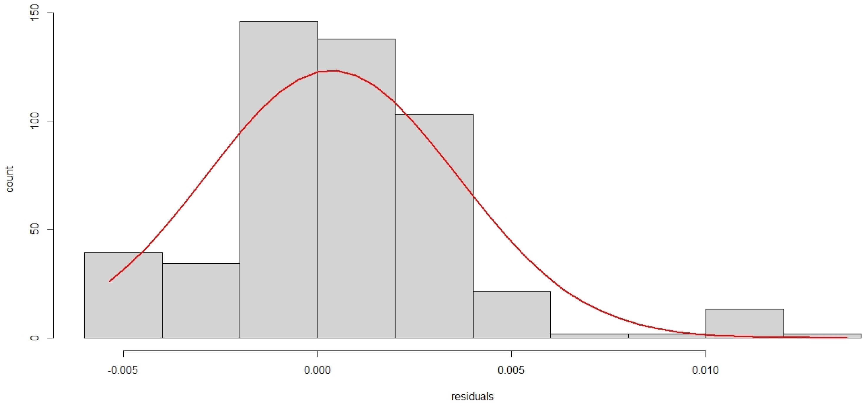


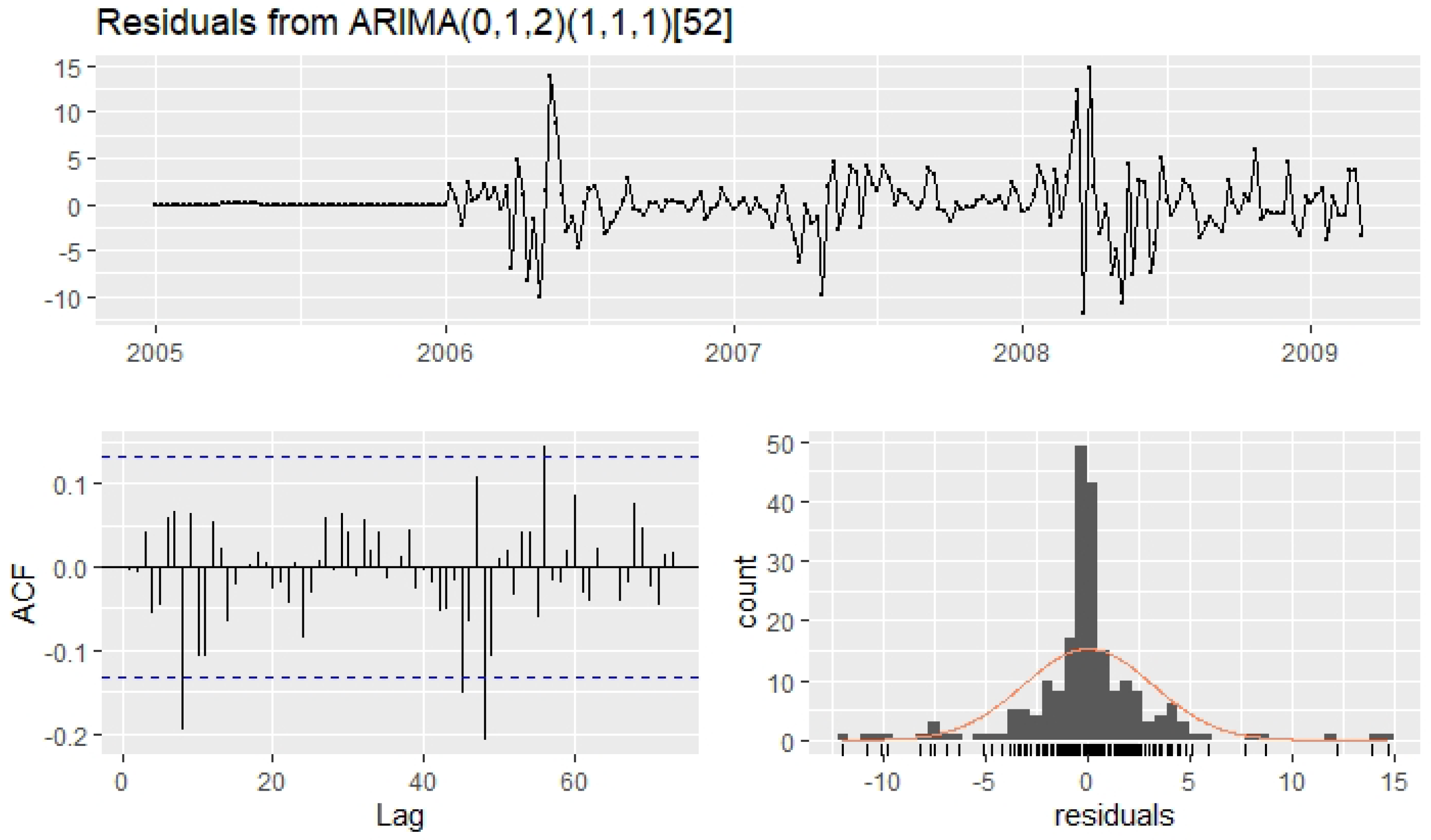
| % Cross Validation | Number of Neurons | Lag | M1 | M2 | M3 | M4 | ||
|---|---|---|---|---|---|---|---|---|
| 50-30-20 | 1 | 1 | −0.06625 | 0.4186 | 0.05620 | 2.4478 | 0.005962 | 0.002204 |
| 1 | 2 | −0.06647 | 0.4233 | 0.06551 | 2.3676 | −0.01516 | 0.01425 | |
| 1 | 3 | −0.06656 | 0.4238 | 0.06378 | 2.3751 | 0.01507 | 0.01408 | |
| 1 | 7 | −0.06522 | 0.4066 | 0.05645 | 2.5136 | −0.005079 | 0.001599 | |
| 1 | 8 | −0.06583 | 0.4134 | 0.05668 | 2.4735 | 0.007022 | 0.003057 | |
| 1 | 15 | −0.06563 | 0.4116 | 0.05936 | 2.4668 | 0.01425 | 0.01259 | |
| 2 | 1 | −0.04646 | 0.2199 | 0.07528 | 4.01955 | 0.0002599 | 0.0004189 | |
| 2 | 2 | −0.04763 | 0.2312 | 0.07582 | 3.8556 | 0.0009351 | 0.00005421 | |
| 2 | 3 | −0.04617 | 0.2170 | 0.07162 | 4.1247 | −0.001043 | 0.0006747 | |
| 2 | 7 | −0.04644 | 0.2188 | 0.06984 | 4.1280 | −0.0001317 | 0.0001076 | |
| 2 | 15 | −0.04631 | 0.2191 | 0.07028 | 4.1143 | 0.00002179 | 0.0000029 | |
| 60-20-20 | 1 | 7 | −0.02968 | 0.05872 | 0.02122 | 19.8959 | 0.03512 | 0.07772 |
| 2 | 7 | −0.01093 | 0.01578 | 0.01860 | 42.6351 | −0.001431 | 0.0001290 | |
| 60-30-10 | 1 | 7 | −0.01261 | 0.03313 | 0.05186 | 13.8169 | −0.008004 | 0.001986 |
| 2 | 7 | −0.006050 | 0.009820 | 0.02584 | 33.7719 | 0.004652 | 0.0006707 | |
| 70-20-10 | 1 | 7 | 0.004080 | 0.008600 | 0.02212 | 28.7379 | −0.009095 | 0.002647 |
| 2 | 7 | 0.0005900 | 0.003810 | 0.01726 | 46.1714 | −0.007490 | 0.001795 |
| % Cross Validation | Order | AICc | ||
|---|---|---|---|---|
| 50-30-20 | 930.17 | 0.4846 | 23.4102 | |
| 60-20-20 | 775.00 | −6.4198 | 57.07765 | |
| 70-20-10 | 548.13 | −1.2039 | 17.3665 | |
| 80-10-10 | 1089.61 | 1.7847 | 18.0898 |
Publisher’s Note: MDPI stays neutral with regard to jurisdictional claims in published maps and institutional affiliations. |
© 2021 by the authors. Licensee MDPI, Basel, Switzerland. This article is an open access article distributed under the terms and conditions of the Creative Commons Attribution (CC BY) license (https://creativecommons.org/licenses/by/4.0/).
Share and Cite
Cogollo, M.R.; González-Parra, G.; Arenas, A.J. Modeling and Forecasting Cases of RSV Using Artificial Neural Networks. Mathematics 2021, 9, 2958. https://doi.org/10.3390/math9222958
Cogollo MR, González-Parra G, Arenas AJ. Modeling and Forecasting Cases of RSV Using Artificial Neural Networks. Mathematics. 2021; 9(22):2958. https://doi.org/10.3390/math9222958
Chicago/Turabian StyleCogollo, Myladis R., Gilberto González-Parra, and Abraham J. Arenas. 2021. "Modeling and Forecasting Cases of RSV Using Artificial Neural Networks" Mathematics 9, no. 22: 2958. https://doi.org/10.3390/math9222958
APA StyleCogollo, M. R., González-Parra, G., & Arenas, A. J. (2021). Modeling and Forecasting Cases of RSV Using Artificial Neural Networks. Mathematics, 9(22), 2958. https://doi.org/10.3390/math9222958


