Numerical Approach for Detecting the Resonance Effects of Drilling during Assembly of Aircraft Structures ^†

Abstract

This paper is devoted to the development of a numerical approach that allows quick detection of the conditions favorable for the beginning of noticeable vibrations during drilling. The main novelty of the proposed approach lies in taking into account the deviations of the assembled compliant parts during non-stationary contact analysis by means of variation simulation. The approaches to stationary analysis of assembly quality are expanded and generalized for modeling such non-stationary effects as vibration and resonance. The numerical procedure is based on modeling the stress–strain state of the assembled structures by solving the corresponding transient contact problem. The use of Guyan reduction, the node-to-node contact model and the application of the generalized α method allow the reformulation of the contact problem in terms of a series of quadratic programming problems. The algorithm is thoroughly tested and validated with commercial software. The efficiency of the developed numerical procedure is illustrated by analysis of the test joints of two aircraft panels. The unsteady process of drilling the panels with periodic drilling force was simulated. The influence of deviations in the shape of the parts on the non-stationary interlayer gap was modeled by setting different initial gaps between parts. It is shown that the oscillation amplitudes of the interlayer gap depend on the initial gaps and do not correlate with the mean value of the stationary residual gap. Thus, non-stationary analysis provides new information about the quality of the assembly process, and it should be applied if the assembly process includes periodic impact on the assembled parts.

1. Introduction

The assembly of a commercial aircraft involves multiple drilling and reaming operations in order to make holes for fastener installation [1,2]. A common hole-producing operation in aircraft assembly is drilling holes through multiple layers of sheet metal or composite materials in order to fasten them together [3,4]. One of the most important conditions to be met during drilling is to ensure that the interlayer gap between the assembled parts is less than the specified value (usually a few tenths of a millimeter). Violation of this condition can lead to problems such as burr formation, ingress of chips between the assembled parts and misalignment of the drilled holes [5,6,7,8].

Nowadays, mathematical modeling is increasingly used to optimize the assembly process [9,10,11]. In particular, the drill loads are taken into account in analysis and optimization of the assembly process [12]. Luo et al. [13] investigated the drilling parameters of Al7075-T6 aerospace aluminum alloy and the chip formation using finite element analysis. Liu et al. [14] optimized the drilling process to reduce the interlayer gap through numerical simulation and experimentation. Tinkloh et al. [15] investigated the effect of composite waviness on the drilling process.

There are a lot of studies devoted to vibration during drilling. Savilov et al. [16] proposed vibration suppression methods. Zhang et al. [17] developed an ambient vibration control system to improve the precision and efficiency of robotic drilling systems. In addition, methods for improving the drilling process using vibrations have been actively developed recently [18,19,20,21]. Therefore, non-stationary modeling of the assembly process, taking into account deviations of the parts, becomes very relevant. At the same time, the software tools for simulation and optimization of the assembly process use stationary contact analysis coupled with variation and statistical analysis [22], and the drilling loads are set as constant. This excludes from consideration the simulation of such phenomena as vibration and resonance, which can occur during drilling. In this paper, an attempt is made to expand the existing methodology for modeling these non-stationary phenomena.

In the numerical analysis of the assembly, it is necessary to take into account the shape variations of the assembled parts caused by manufacturing discrepancies, fixation tolerances, etc. The accounting for compliance of the parts can be performed with finite element modeling. Liu and Hu proposed the method of influence coefficients (MIC) [23], which takes into account the elastic properties of the parts in variation analysis and springback calculation by using the pre-calculated reduced stiffness matrices. The classic MIC approach assumes that the interaction between the parts occurs only in special predefined points of fastening (e.g., welding points). This assumption is justified in many cases, but sometimes it is necessary to take into account that contact can occur at points that are not known in advance. Finding the contact points makes the analysis much more complicated because it requires solving a nonlinear contact problem. The MIC approach, combined with the direct algorithm of the contact point location, was used by Wärmefjord et al. in [24] for variation simulation in the automotive industry.

The approach based on reformulation of the contact problem in terms of quadratic programming is presented in [25]. In this paper, the variational formulation of the contact problem [26,27,28,29] is combined with implementation of a reduced stiffness matrix by using the substructuring technique (also known as Guyan reduction) [30,31,32,33]. The approach presented in [25] has been further developed and provided with practical examples in subsequent works by the same authors [22,34]. A similar approach was used by Lorin et al. [35] for simulating the assembly process in the automotive industry.

This work is devoted to the further development and extension of the numerical technique proposed in [25] for modeling and predicting the non-stationary effects that can occur during the assembly of aircraft structures. These effects include the vibration and resonance that can happen during drilling. This article also considers an example of the application of the developed technique to the simulation of drilling of the test joint and the study of accompanying vibrations with regard to variations in part shape.

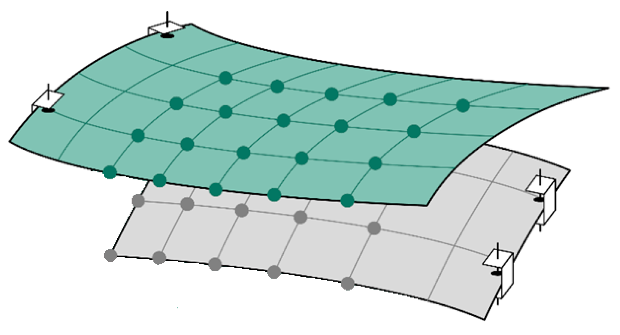
2. Numerical Approach

Figure 1 presents a sketch of a finite element model (FEM) of the assembly of two parts. An FEM consisting of a shell and bar elements is considered. The area of possible contact is called the junction area. Outside this area, there is no contact between the parts. The computational nodes in the junction area are marked with circles in Figure 1.

The variables of the contact problem are all degrees of freedom (DOFs) of the FEM which form a vector-valued function $U\left(t\right)={\left\{U_i\left(t\right)\right\}}_{i=1}^{N_{DOF}},$ where $N_{DOF}$ is the number of DOFs of the model and $t\in \left(0,T\right]$ is the time.

If the possibility of contact interaction of the parts is not taken into account, the vector-valued function $U\left(t\right)$ obeys the equation of linear structural dynamics:

$$M\cdot \ddot{U}\left(t\right)+B\cdot \dot{U}\left(t\right)+K\cdot U\left(t\right)=F\left(t\right),t\in \left(0,T\right],$$

(1)

where $M, B$ and $K$ are the matrices of mass, damping and stiffness, respectively (size $N_{DOF}\times N_{DOF}$), $F\left(t\right)$ is the vector of the applied load (a given function of time) and the superscript dots mean differentiations in time.

The initial conditions for Equation (1) are

$$U\left(0\right)=U_0; \dot{U}\left(0\right)=V_0$$

(2)

where $U_0$ and $V_0$ are the given vectors of the initial displacement and velocity, respectively.

The compliant parts are fixed in the assembly jig (e.g., using clamps, as in Figure 1), so some DOFs are restricted, particularly to avoid the rigid body motion of each part:

$$U_i\left(t\right)=0,i\in {\Gamma }_{fix},\forall t\in \left(0,T\right]$$

(3)

where ${\Gamma }_{fix}$is the set of indices of nodes with restricted degrees of freedom.

It is assumed that the finite element meshes of the parts are conformal in the junction area, so the node-to-node contact model can be used. This means that the pairs of possible contact nodes are predefined. The time-independent vector of the initial gap $G={\left\{g_i\right\}}_{i=1}^{N_{NC}}$ determines the constraints on the displacements of the parts. The non-penetration condition of Equation (4) has also been added to the system of Equations (1)–(3):

$$A\cdot U\left(t\right)\le G,\forall t\in \left(0,T\right],$$

(4)

where $A$ is a time-independent matrix of size $N_{NC}\times N_{DOF}$ defining the constraints in the nodes.

The system of Equations (1)–(4) corresponds to a contact problem with continuous time. The dimension of the problem is equal to the number of all degrees of freedom of the assembly provided by the FEM, which can reach ${10}^6-{10}^7$ variables for industrial applications. It makes this formulation of the contact problem inapplicable if serial calculations are required (e.g., variation simulation or assembly optimization) [36]. Guyan reduction [30,31] is used for the reduction of the problem dimension. This approach has been successfully applied to solving static assembly problems (see [34,37]).

2.1. Guyan Reduction

After renumbering, the vector of all DOFs can be represented as follows:

$$U=\left(\begin{array}{c}{U}_C\\ U_R\end{array}\right)$$

where $U_C$ is the vector of those degrees of freedom in the junction area that are constrained by Equation (4). All other DOFs form the vector $U_R$. The global stiffness matrix K can also be represented in the form of corresponding blocks:

$$K=\left(\begin{array}{cc}{K}_{CC}& K_{CR}\\ K_{CR}^T& K_{RR}\end{array}\right).$$

The mass matrix $M$, damping matrix $B$ and load vector $F$ can be subdivided in the same way. Then, Equation (1) can be rewritten as

$$\left(\begin{array}{cc}{M}_{CC}& M_{CR}\\ M_{CR}^T& M_{RR}\end{array}\right)·\left(\begin{array}{c}{\ddot{U}}_C\\ {\ddot{U}}_R\end{array}\right)+\left(\begin{array}{cc}{B}_{CC}& B_{CR}\\ B_{CR}^T& B_{RR}\end{array}\right)·\left(\begin{array}{c}{\dot{U}}_C\\ {\dot{U}}_R\end{array}\right)+\left(\begin{array}{cc}{K}_{CC}& K_{CR}\\ K_{CR}^T& K_{RR}\end{array}\right)·\left(\begin{array}{c}{U}_C\\ U_R\end{array}\right)=\left(\begin{array}{c}{F}_C\\ F_R\end{array}\right).$$

(5)

Usually in the assembly problems, there are no loads outside the junction area, and therefore $F_R=0$. As such, when excluding $U_R$ from Equation (5), the following equation for $U_C$ is obtained:

$$\begin{array}{l}\left(M_{CR}-K_{CR}\cdot K_{RR}^{-1}\cdot M_{RR}\right)\cdot {\ddot{U}}_R+\left(B_{CR}-K_{CR}\cdot K_{RR}^{-1}\cdot B_{RR}\right)\cdot {\dot{U}}_R+\left(M_{CC}-K_{CR}\cdot K_{RR}^{-1}\cdot M_{CR}^T \right)\\ \cdot {\ddot{U}}_C+\left(B_{CR}-K_{CR}\cdot K_{RR}^{-1}\cdot K_{CR}^T\right)\cdot {\dot{U}}_C+\left(K_{CC}-K_{CR}\cdot K_{RR}^{-1}\cdot K_{CR}^T\right)\cdot U_C\\ =F_C.\end{array}$$

(6)

It is assumed that the first and the second terms in Equation (6) can be neglected. Reduced matrices of the mass, damping and stiffness are also introduced:

$$\begin{gathered} M_C≔\left(M_{CC}-K_{CR}\cdot K_{RR}^{-1}\cdot M_{CR}^T\right), \\ {B}_C≔\left(B_{CR}-K_{CR}\cdot K_{RR}^{-1}\cdot K_{CR}^T\right), \\ {K}_C≔\left(K_{CC}-K_{CR}\cdot K_{RR}^{-1}\cdot K_{CR}^T\right). \end{gathered}$$

Then, the main equation of the original problem (Equation (1)) can be rewritten as follows:

$$M_C\cdot {\ddot{U}}_C\left(t\right)+B_C\cdot {\dot{U}}_C\left(t\right)+K_C\cdot U_C\left(t\right)=F_C\left(t\right), t\in \left(0,T\right].$$

(7)

The contact problem with Equation (7) involves only constrained DOFs. Therefore, the dimension of this problem is much smaller than the original contact problem with Equation (1). Thus, this problem formulation is more suitable for the serial calculations. Note that there are various ways to reduce the mass and damping matrices, which are described in detail, for example, in [38]. Furthermore, only the reduced problem is discussed; therefore, for simplicity, the subscript $C$ is omitted in Equation (7).

2.2. Time Discretization Algorithm

For discretization of Equation (7) in the time domain, a time grid $t_n=n\mathsf{\Delta }t$ is introduced, with $n=0,\dots ,N_T$ and $\mathsf{\Delta }t=T/N_T$ and denoting $U_n:=U\left(t_n\right)$. The generalized α method proposed in [39] is used. The discrete velocity $V_n$ and acceleration $W_n$ are calculated by the following formulas in accordance with the generalized α method:

$$V_{n+1}=\frac{1}{\gamma \mathsf{\Delta }t}\left(U_{n+1}-U_n\right)+\left(1-\frac{1}{\gamma }\right)V_n+\mathsf{\Delta }t\left(1-\frac{1}{2\gamma }\right)W_n,$$

(8)

$$W_{n+1}=\frac{1}{\alpha \mathsf{\Delta }{t}^2}\left(U_{n+1}-U_n\right)-\frac{1}{\alpha \mathsf{\Delta }t}{V}_n+\left(1-\frac{1}{2\alpha }\right)W_n.$$

(9)

Here, $\gamma$ and $\alpha$ are the parameters of the generalized α method that define the contribution of the $n$ and $\left(n+1\right)$time layers in the numerical scheme. Introducing the parameters κ and φ allows one to suppress the unwanted high-frequency noise during time integration. Finally, the system in Equation (10) is obtained:

$$D\cdot U_n=C_n, n=1,\dots ,N_T.$$

(10)

This can be considered a system of equations of the static contact problem with the equivalent matrix of stiffness

$$D=\frac{1-\kappa }{\alpha \mathsf{\Delta }{t}^2}M+\frac{1-\phi }{\gamma \mathsf{\Delta }t}B+\left(1-\phi \right)K$$

(11)

and the equivalent load vector

$$\begin{gathered} C_{n+1}=\left(1-\phi \right)F\left(t_{n+1}\right)+\phi F\left(t_n\right)-\phi K\cdot U_n+ \\ M\cdot \left(\frac{1-\kappa }{\alpha \mathsf{\Delta }{t}^2} U_n+\frac{1-\kappa }{\alpha \mathsf{\Delta }t}{V}_n+\left(\frac{1-\kappa }{2\alpha }-1\right)W_n\right)+ \\ B\cdot \left(\frac{1-\phi }{\gamma \mathsf{\Delta }t}{U}_n+\left(\frac{1-\phi }{\gamma }-1\right)V_n+\mathsf{\Delta }t\left(1-\phi \right)\frac{\left(1-2\gamma \right)}{2\gamma } W_n\right). \end{gathered}$$

(12)

If the time step $\mathsf{\Delta }t$ is constant, the matrix $D$ does not change between steps. The load vector $C_n$ depends on the displacement, velocity and acceleration in the previous layer.

If the parameters satisfy the following conditions

$$\begin{gathered} \frac{\alpha }{\gamma }=\frac{1}{2}-\kappa +\phi , \\ \kappa \le \phi \le \frac{1}{2}, \\ \alpha \ge \frac{1}{4}+\frac{1}{2}\left(\phi -\kappa \right) \end{gathered}$$

then the generalized α method is unconditionally stable and has the second order of accuracy [39].

The system in Equation (10) with the conditions of Equations (2)–(4) for $U_n$ determines the non-linear contact problem on the time layer n. Let us formulate this problem in variational form [40] by finding the minimizer of the functional

$$\begin{gathered} \min \left\{\frac{1}{2}{U}_n^T\cdot D\cdot U_n-C_n^T\cdot U_n\right\} \\ \mathrm{subject} \mathrm{to} A\cdot U_n\le G \end{gathered}$$

(13)

at every time layer $n=1,\dots ,N_T$. The initial conditions for this problem are defined in Equation (2).

2.3. Basic Assumptions of the Numerical Algorithm

To summarize this section, the main assumptions of the numerical approach are listed and discussed here.

Shell and bar elements are used to build the finite element model. The fastener and drilling loads are defined as time-dependent point forces normal to the contact surface. The indicated simplifications are accepted due to the fact that the described approach is intended for modeling the assembly of large-scale aircraft structures (e.g., wing panels, fuselage sections and final aircraft assembly).

The deformation of each part in the assembly is described by the linear elasticity theory. The contact interaction between the parts without friction is taken into account. Only displacements of parts in the normal direction (to the contact surface) are modeled. A node-to-node contact model is used. These assumptions are justified, since the installed fasteners prevent significant relative tangential displacement of the parts. In addition, this work is devoted to the study of opening the gap between parts when drilling. Only normal displacements can lead to such an opening.

When modeling the non-stationary processes, the inertia and damping of the assembled parts outside the junction area are neglected. At the same time, inside the junction area, these effects are taken into account in full. This assumption makes it possible to significantly reduce the dimension of the problem by performing the Guyan reduction procedure. As a rule, the clamping of parts to the assembly stand eliminates noticeable movements (and, consequently, accelerations) of parts outside the junction area, which makes it possible to neglect the inertial effects in this area. If for some reason the inertial effects outside the junction area need to be accounted for, the developed approach cannot be applied directly and needs to be modified.

The developed approach is designed to analyze the assembly process, taking into account the deviations of the shape of the assembled parts from the nominal. Modeling of the deviations is carried out by generating the random uneven initial gaps between the parts using the stochastic methods [34]. The analysis of the influence of the part deviations is carried out by the massive solving of non-stationary contact problems and the subsequent statistical analysis of the obtained results.

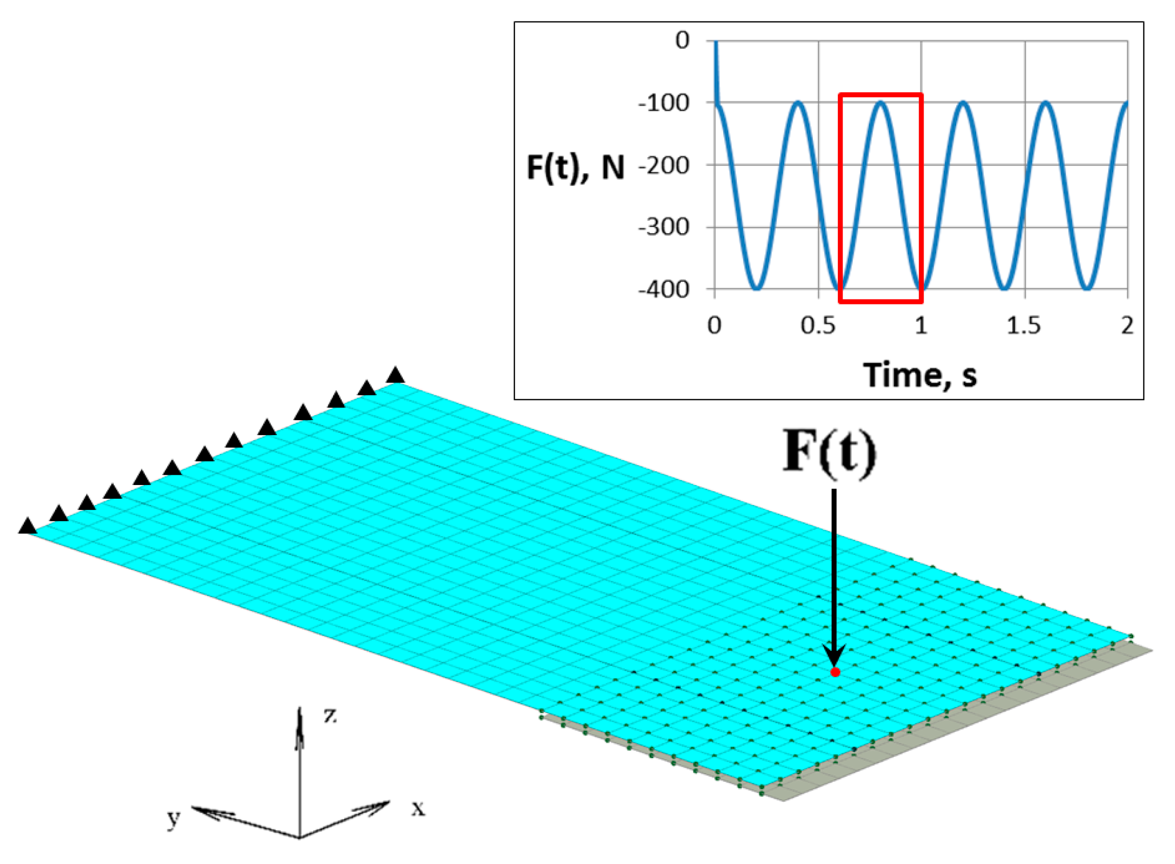
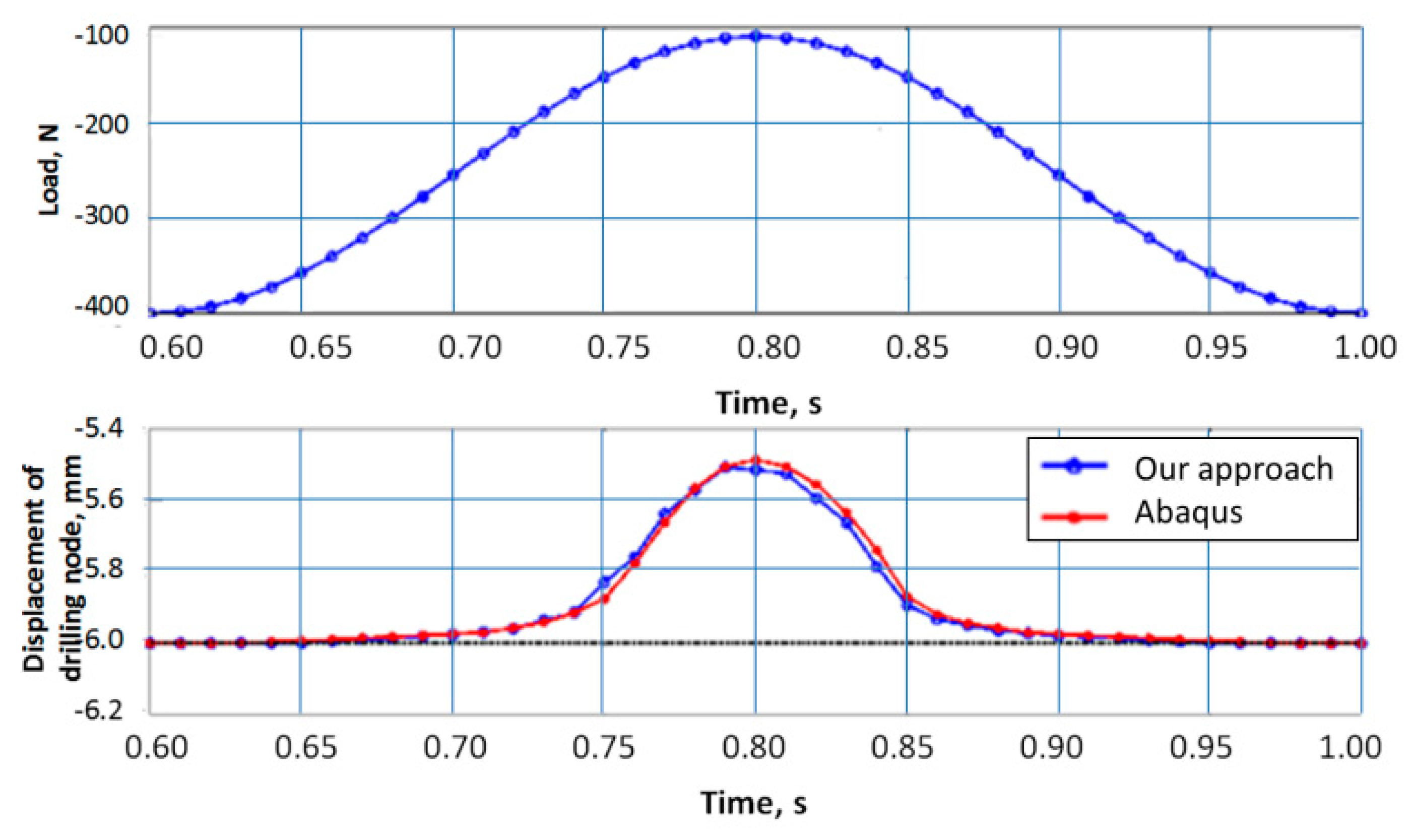
3. Verification with Abaqus

This section is devoted to verification of the proposed approach with the commercial code Abaqus FEA (see [41] for details). A simplified assembly model was used for this. The assembly consisted of two parts: a compliant rectangular panel and a fixed absolutely rigid obstacle. The upper part was fixed to the rear edge (Figure 2). It was modeled by the shell finite elements. A constant initial gap between parts was considered here, which equaled 6 mm everywhere in the junction area. A time-dependent harmonic load was applied to the top panel in the middle of the junction area (see Figure 2). The calculations were carried out for t from 0 to 2 s with a time step $\mathsf{\Delta }t={10}^{-2}$ s.

A comparison of the solution with Abaqus is presented for the vertical displacement of the node to which the drilling load was applied. The time interval from 0.6 s to 1 s corresponds to the time period. The displacements for this time interval are shown in Figure 3. It can be seen that the two solutions were close to each other. The slight time shift was apparently caused by inaccuracies in the reduction of the mass matrix.

Note that the upper panel came into contact with the obstacle at times $t=0.6$ s and $t=1$ s (the position of the obstacle is shown in Figure 3 (below) with a black line).

The computation time with Abaqus was 55.3 s, while the developed numerical procedure solved the problem in 1.2 s (excluding the time required to compute the reduced matrices). The problem was solved on a PC with an Intel Core i5 processor (3.60 GHz) and 16 GB of RAM running Windows 10. This significant speedup makes it possible to use the developed approach in variation analysis, which implies multiple computations with different input parameters.

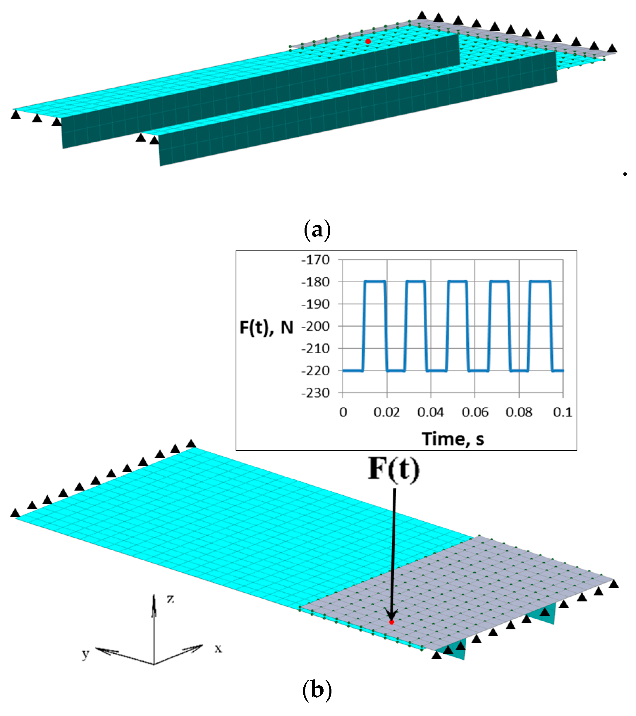
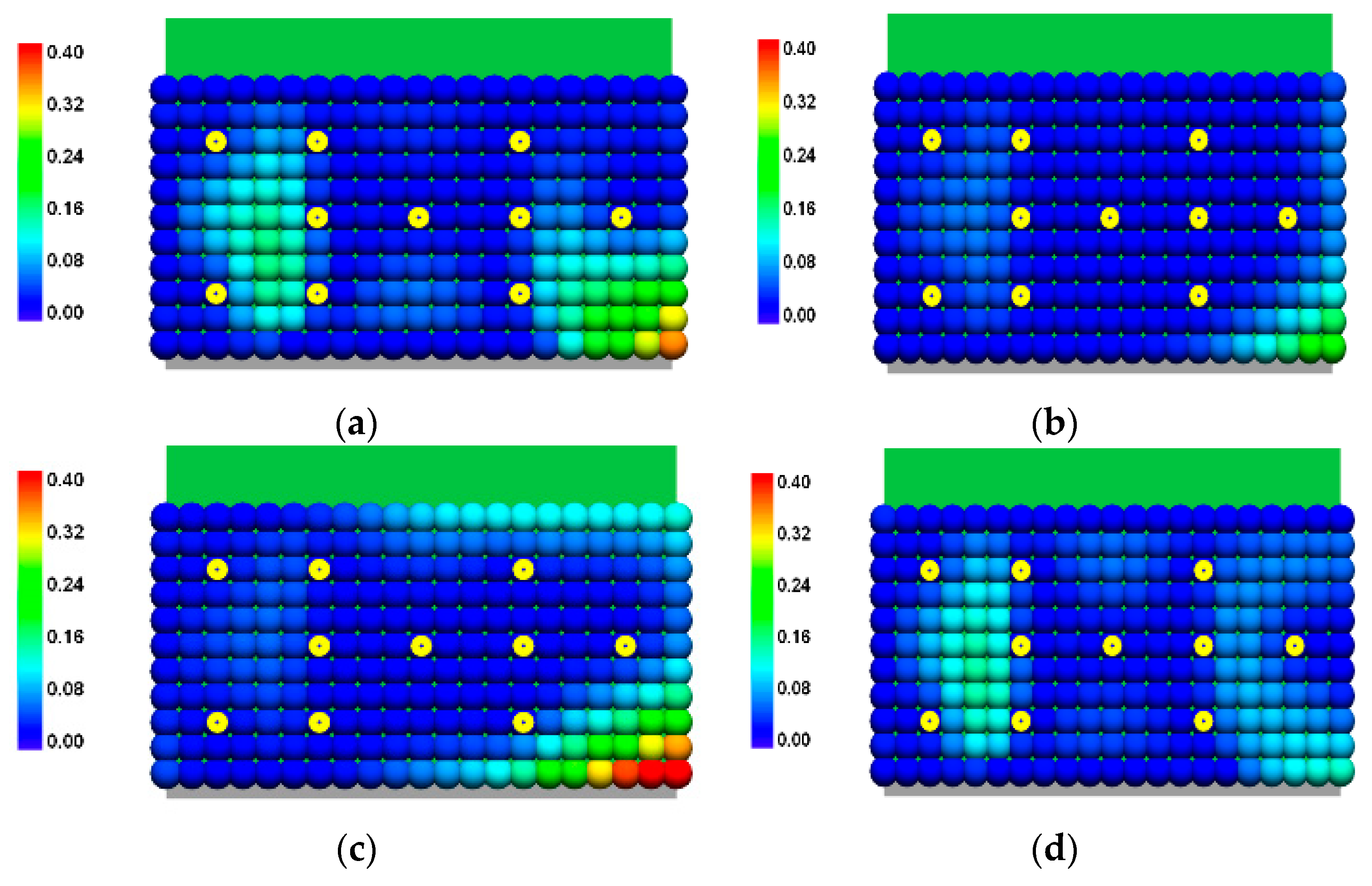
4. Drilling Process Simulation

The considered model of assembly of two compliant panels is shown in Figure 4. The geometrical and mechanical parameters of the assembly were selected to imitate the part of the wing-to-fuselage joint of an aircraft. The lower panel was reinforced with two stringers (see Figure 4a). The thickness was 5 and 10 mm for the lower and upper panels, respectively. The finite element model consisted of the shell elements. The fixed edges are marked in Figure 4 with black triangles. All displacements and rotations were forbidden in all nodes of the marked edges. The panels were made of Al2024 aluminum alloy. The elastic modulus was 73 GPa, the Poisson ratio was 0.33, and the density was 2780 kg/m³. The junction area is depicted with green points in Figure 4. There were 231 nodes in the junction area of each part.

The calculation of the reduced matrices $M_C$, $B_C$ and $K_C$ was carried out in MSC Nastran FEA code. For solving the quadratic programming problem (Equation (13)), the interior point method in MATLAB was used.

In the assembly, there were 15 holes for fastener installation (see Figure 5). Ten temporary fasteners were installed in the holes marked with yellow circles in Figure 5. As is shown in [42], the load in the temporary fasteners could be considered constant. The load in each fastener was set to 5000 N and applied to both panels as presented in Figure 5.

The panels were drilled from top to bottom. The interlayer gap was maximal when the upper panel had already been drilled and the bottom one was starting to be drilled. It was this case that was modeled in the example under consideration. The drilling load acted on the lower panel at the point marked with a red circle in Figure 4b and Figure 5. At this point, a piecewise constant periodic load was applied with a frequency of 53.05 Hz, corresponding to the rotation speed of the drill (see the graph in Figure 4).

The simulation was carried out for a time interval from 0 to 0.5 s. The time step$\Delta t$ was chosen to be equal to ${10}^{-4}$ s. Four random initial gaps [34] were considered to illustrate the combination of transient contact analysis and variation simulation.

The nodes of the computation mesh colored by initial gaps are plotted in Figure 6.

The initial conditions for the transient simulation corresponded to the stress–strain state of the assembly with installed fastening elements. The displacements $U_0$ were obtained by solving the static problem with applied constant loads from the fasteners. The initial velocities $V_0$ were taken as equal to zero. The residual gaps between pars after installation of the fastening elements are presented in Figure 7.

The aim of the simulation was to compare the oscillation amplitudes of the residual gap $g_{drill}\left(t\right)$ between the panels at the drilling point for the different initial gaps. The time dependencies of the gap are shown in Figure 8 in the time interval from 0.3 s to 0.5 s. The green dashed lines in these figures represent the mean values of the gap.

The values of the mean residual gap and the amplitudes of the periodic oscillations (calculated as half the difference between the maximum and minimum) are presented in

Table 1. Parameters of the residual gap in the drilling point.

Initial Gap	Mean Residual Gap (μm)	Mean Amplitude (μm)
$G_1$	137.0	6.4
$G_2$	102.7	7.6
$G_3$	112.5	8.6
$G_4$	138.0	7.7

for each initial gap. It can be seen that the oscillation amplitudes depended on the initial gaps and did not correlate with the mean value of the residual gap. Consequently, non-stationary analysis can provide new information about the quality of the assembly process compared with stationary analysis.

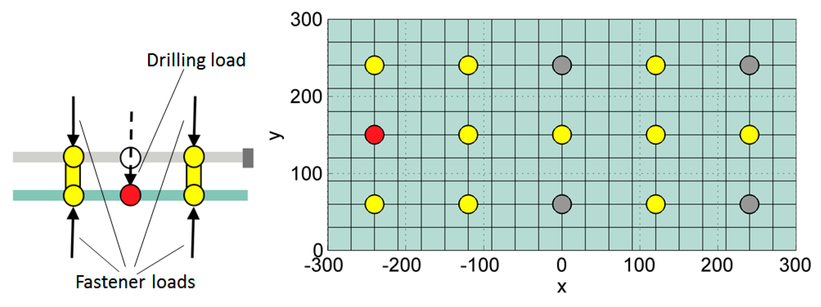
5. Search for Resonance Effects

This section focuses on finding possible resonance effects that can arise during the drilling process and cause dangerous vibration of the parts. This is performed by determining the natural frequencies of the assembly and testing different drilling frequencies in their neighborhood. As the stress–strain state of the assembly is controlled by the initial gap between the parts and installed fastening elements, all these factors need to be included in the analysis. Therefore, the previously described procedure for transient contact analysis was used as the main research tool.

Since it is advisable to look for resonance effects in the neighborhood of the natural frequencies, further calculations were aimed at finding them.

5.1. Determination of Natural Frequencies

The considered process was nonlinear due to the contact interaction in the assembly, and the gap between the parts could be opened and closed during drilling. Therefore, the standard technique for determination of the natural frequencies by modal analysis was not applicable here. Therefore, a different approach was used based on Fourier analysis of the system response to a sudden perturbation, which is commonly employed for examination of nonlinear systems.

Here is a brief description of the numerical algorithm:

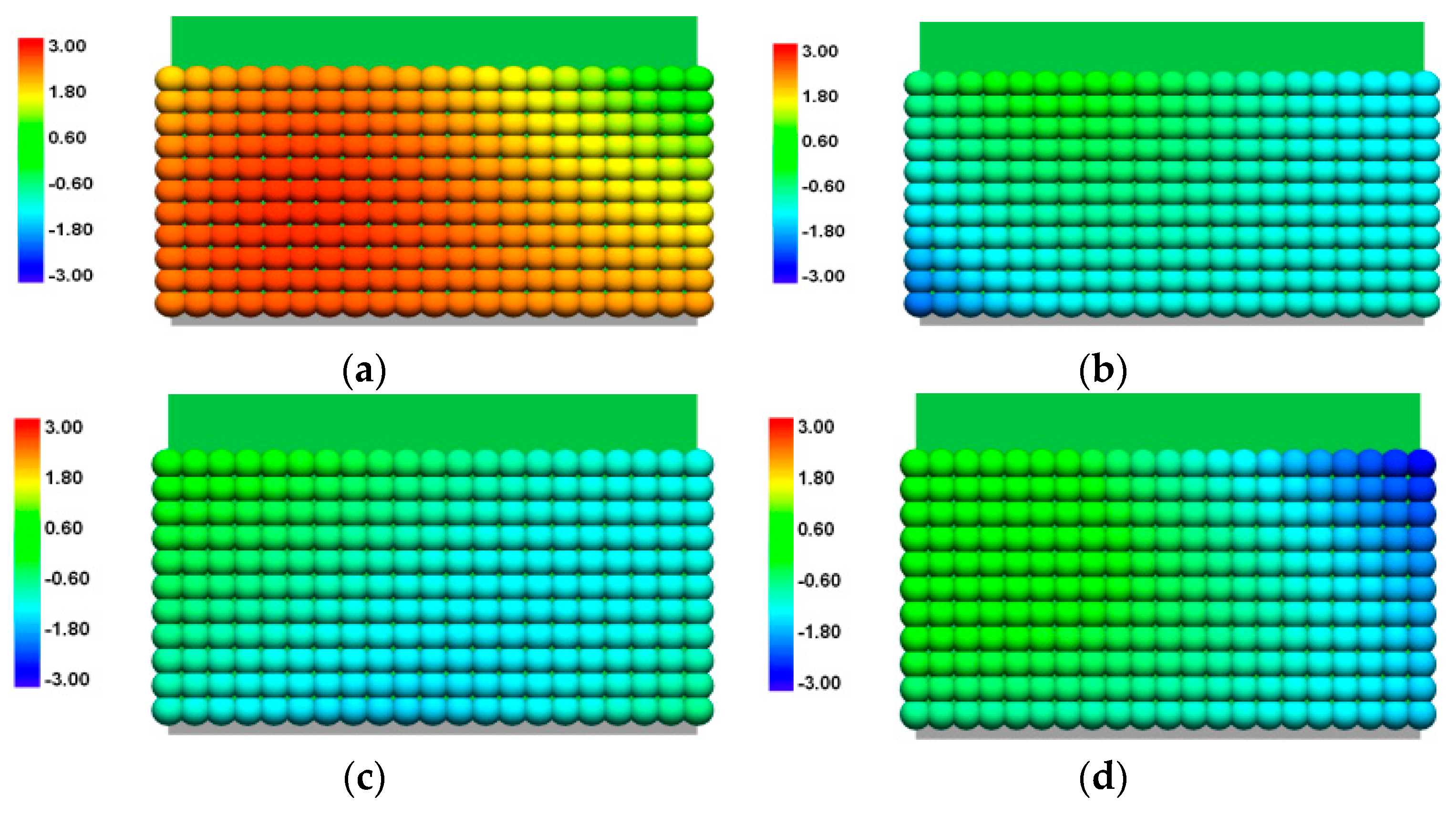
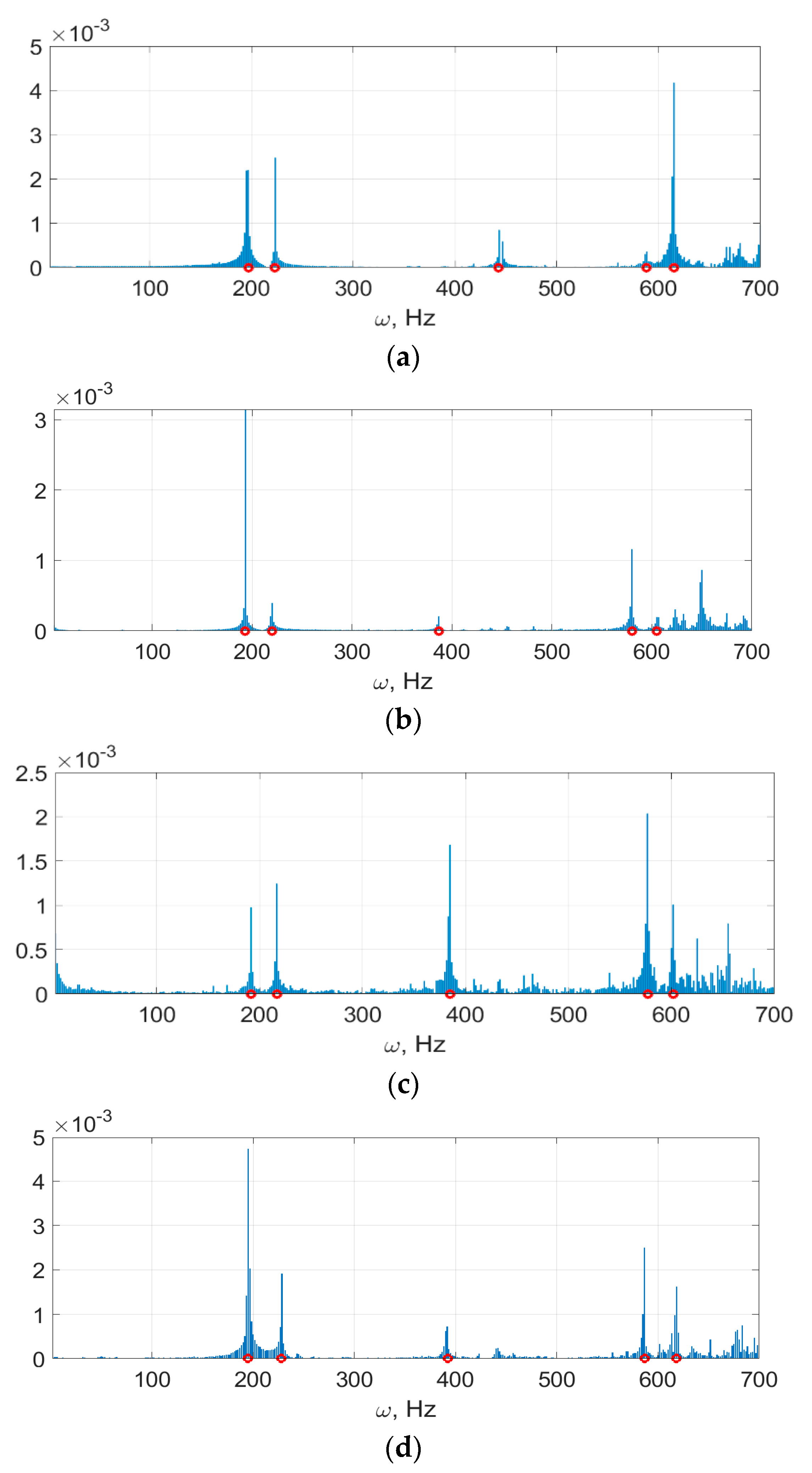
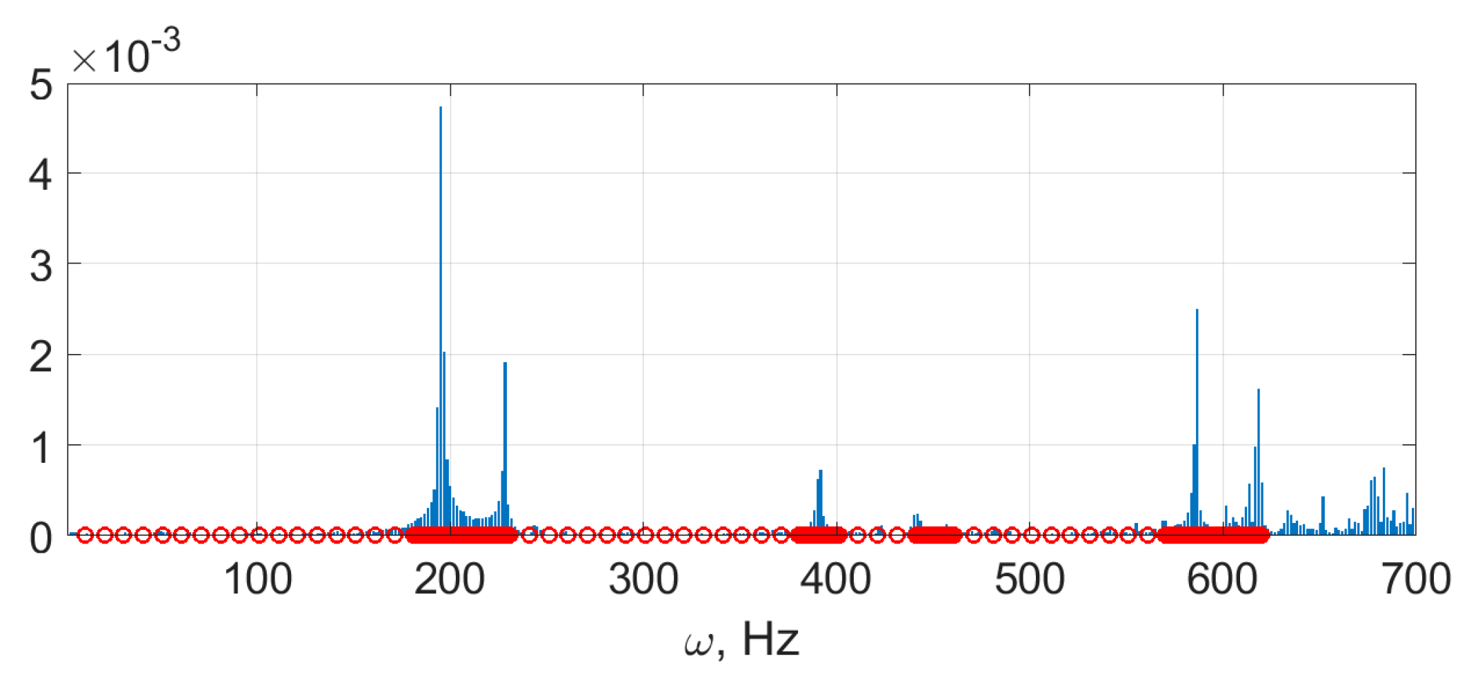
• The upper panel is affected by a sudden impulse to the drilling node (indicated by the red circle in Figure 5). The impulse causes free oscillations of both panels in the assembly. The damping is set to zero, so the oscillations do not decay. These oscillations are simulated by solving Equation (13) with initial conditions corresponding to the installed fasteners, as it was described in the previous section.
• The frequency response function $A_g^{free}\left(\omega \right)$ is obtained as a Fourier transform of the computed residual gap in the drilling node.
• The natural frequencies ${\omega }_{NF}$ of the assembly correspond to the local maxima of $A_g^{free}\left(\omega \right)$.

The natural frequencies are calculated on a time grid with parameters $\mathsf{\Delta }t=5\times {10}^{-4}$ s and $T=1$ s. These parameters allow for obtaining the natural frequencies in the interval between ${\omega }_{min}=10$ Hz and ${\omega }_{max}=1000$ Hz.

The resulting frequency response functions obtained by the algorithm described above are shown in Figure 9 for different initial gaps. The first five natural frequencies are marked by red rings in Figure 9 and are listed in

Table 2. Natural frequencies for different initial gaps.

Initial Gap	Natural Frequencies (Hz)
$G_2$	193	220	387	580	615
$G_1$	197	223	443	588	605
$G_3$	192	217	385	577	602
$G_4$	195	228	392	587	618

in ascending order. As can be seen, the calculated natural frequencies depend, although not very strongly, on the initial gap.

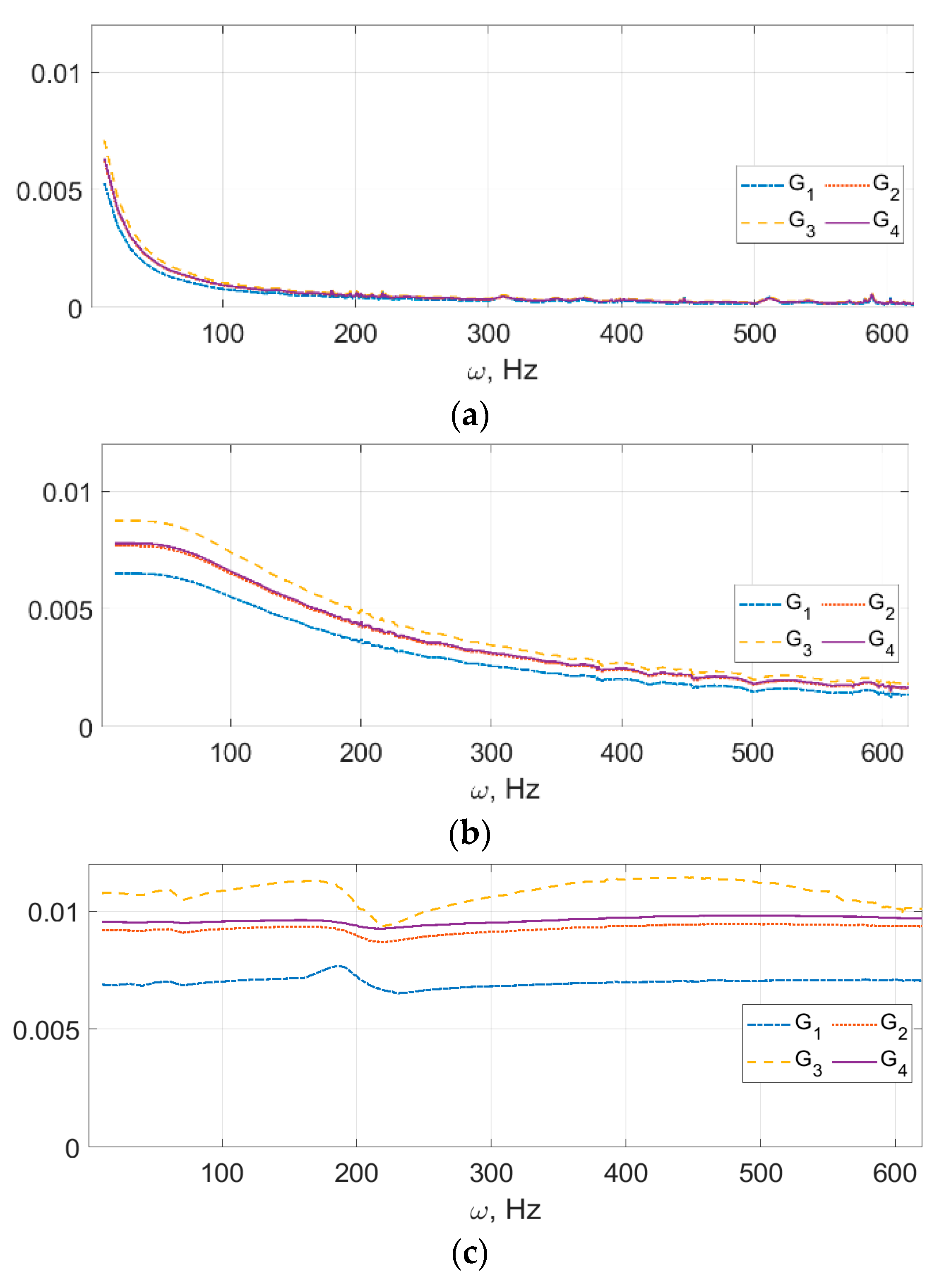
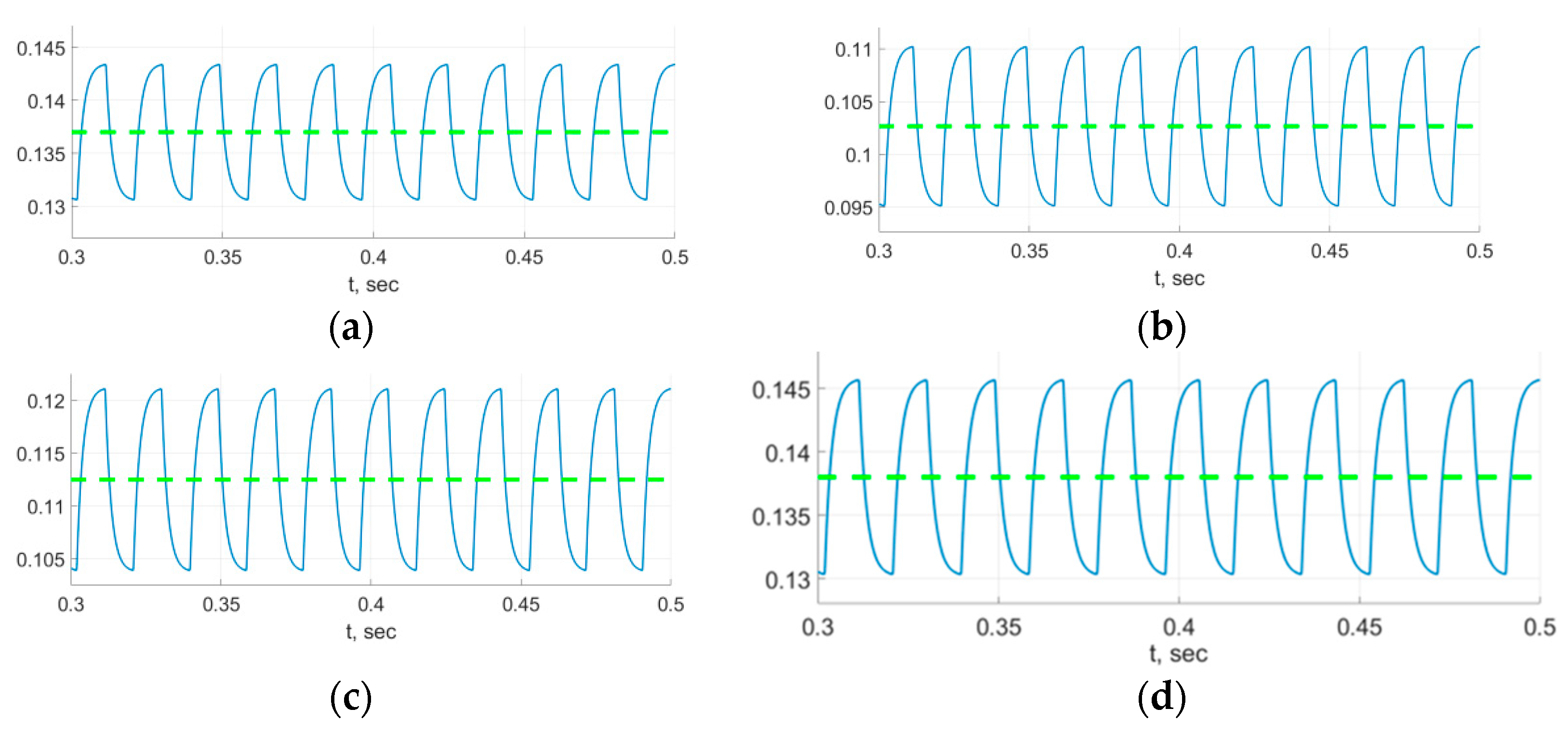
5.2. Building the Dependence of the Vibration Amplitude on the Drill Rotational Speed by Massive Computations

The various drilling frequencies with different initial gaps between parts and damping parameters are investigated here.

Let us define a mesh in a frequency domain that consists of 200 nodes and condenses near the natural frequencies as shown in Figure 10.

In this type of task, it is quite difficult to set the damping of the system correctly. Usually, this parameter is determined by experimentation on a real physical structure. The original damping matrix $B$ was calculated with Nastran as the weighted sum of the mass and stiffness matrices [43]:

$$B={\alpha }_{M}M+{\alpha }_{K}K,$$

where ${\alpha }_M$ is the Rayleigh damping mass matrix scale factor and ${\alpha }_K$ is the Rayleigh damping stiffness matrix scale factor. In order to test the influence of damping on the solution, the factors $b_1>b_2>b_3$ were introduced before the damping matrix $B$:

$$b_n={10}^{-n}, n=1, 2, 3.$$

For each drilling frequency shown in Figure 10, the simulation of the drilling process was performed in the same way as described in Section 4. The four initial gaps (shown in Figure 6) and the three damping coefficients $b_{1,2,3}$ were considered. In total, 2400 transient contact simulations were performed, and the residual gap between panels $g_{drill}$ was computed in all cases. The resulting dependencies of the $g_{drill}$ oscillation amplitude on the drilling load frequency are plotted in Figure 11. As can be seen from Figure 11a,b, all high-frequency oscillations were damped with large damping coefficients. Even with small damping (Figure 11c), the large oscillation amplitudes of the residual gap were not detected in the full range of drilling load frequencies (including the neighborhood of the natural frequencies).

6. Conclusions

This paper presents a methodology for determining potentially dangerous frequencies for drilling, at which a gap between the parts to be joined may open. This effect depends on the initial gap between the parts, as well as the location and properties of the fasteners.

In the examined virtual test assembly, the significant increase in the residual gap between parts was not observed in the whole considered range of drilling frequencies. This was due to the fact that in the considered example, the elastic forces dominated over the inertial ones, and noticeable resonance effects did not appear. As a rule, the resonance effects during drilling are also not revealed in industrial aircraft production. However, there is a possibility that this effect can come out in some particular cases. This should be avoided, as it can cause the injection of drilling cuttings between the contact surfaces of parts, which is considered extremely undesirable when assembling aircraft structures. Thus, it seems to be important to equip the software tools for modeling the assembly process of aircraft structures (such as ASRP [22]) with special modules to determine potentially dangerous resonance effects during drilling. Such modules can work according to the technique described in this work.

References

1. Aamir, M.; Tolouei-Rad, M.; Giasin, K.; Nosrati, A. Recent advances in drilling of carbon fiber–reinforced polymers for aerospace applications: A review. Int. J. Adv. Manuf. Technol. 2019, 105, 2289–2308. [Google Scholar] [CrossRef]
2. Aamir, M.; Giasin, K.; Tolouei-Rad, M.; Vafadar, A. A review: Drilling performance and hole quality of aluminium alloys for aerospace applications. J. Mater. Res. Technol. 2020, 9, 12484–12500. [Google Scholar] [CrossRef]
3. Bañon, F.; Sambruno, A.; Fernandez-Vidal, S.; Fernandez-Vidal, S.R. One-Shot Drilling Analysis of Stack CFRP/UNS A92024 Bonding by Adhesive. Materials 2019, 12, 160. [Google Scholar] [CrossRef] [Green Version]
4. Hassan, M.H.; Abdullah, J.; Franz, G.; Shen, C.Y.; Mahmoodian, R. Effect of Twist Drill Geometry and Drilling Parameters on Hole Quality in Single-Shot Drilling of CFRP/Al7075-T6 Composite Stack. J. Compos. Sci. 2021, 5, 189. [Google Scholar] [CrossRef]
5. Melkote, S.N.; Newton, T.R.; Hellstern, C.; Morehouse, J.B.; Turner, S. Interfacial Burr Formation in Drilling of Stacked Aerospace Materials. In Burrs—Analysis, Control and Removal; Aurich, J.C., Dornfeld, D., Eds.; Springer: Berlin/Heidelberg, Germany, 2010; pp. 89–98. ISBN 978-3-642-00567. [Google Scholar]
6. Giasin, K.; Ayvar-Soberanis, S. An investigation of burrs, chip formation, hole size, circularity and delamination during drilling operation of GLARE using ANOVA. Compos. Struct. 2017, 159, 745–760. [Google Scholar] [CrossRef]
7. Habib, N.; Sharif, A.; Hussain, A.; Aamir, M.; Giasin, K.; Pimenov, D.Y.; Ali, U. Analysis of Hole Quality and Chips Formation in the Dry Drilling Process of Al7075-T6. Metals 2021, 11, 891. [Google Scholar] [CrossRef]
8. Lee, J.H.; Ge, J.C.; Song, J.H. Study on Burr Formation and Tool Wear in Drilling CFRP and Its Hybrid Composites. Appl. Sci. 2021, 11, 384. [Google Scholar] [CrossRef]
9. Xi, F.-F.; Yu, L.; Tu, X.W. Framework on robotic percussive riveting for aircraft assembly automation. Adv. Manuf. 2013, 1, 112–122. [Google Scholar] [CrossRef] [Green Version]
10. Ni, J.; Tang, W.C.; Pan, M.; Qiu, X.; Xing, Y. Assembly sequence optimization for minimizing the riveting path and overall dimensional error. In Proceedings of the Institution of Mechanical Engineers, Part B: Journal of Engineering Manufacture; SAGE Publications: Thousand Oaks, CA, USA, 2018; Volume 232, pp. 2605–2615. [Google Scholar]
11. Gulivindala, A.K.; Bahubalendruni, M.R.; Varupala, S.V.P.; Sankaranarayanasamy, K. A heuristic method with a novel stability concept to perform parallel assembly sequence planning by subassembly detection. Assem. Autom. 2020. [Google Scholar] [CrossRef]
12. Lupuleac, S.; Shinder, J.; Churilova, M.; Zaitseva, N.; Khashba, V.; Bonhomme, E.; Montero-Sanjuan, P. Optimization of Automated Airframe Assembly Process on Example of A350 S19 Splice Joint. SAE Tech. Pap. 2019. [Google Scholar] [CrossRef]
13. Luo, H.; Fu, J.; Wu, T.; Chen, N.; Li, H. Numerical Simulation and Experimental Study on the Drilling Process of 7075-t6 Aerospace Aluminum Alloy. Materials 2021, 14, 553. [Google Scholar] [CrossRef] [PubMed]
14. Liu, J.; Zhao, A.; Wan, P.; Huiyue, D.; Yunbo, B. Modeling and Optimization of Bidirectional Clamping Forces in Drilling of Stacked Aluminum Alloy Plates. Materials 2020, 13, 2866. [Google Scholar] [CrossRef]
15. Tinkloh, S.; Wu, T.; Tröster, T.; Niendorf, T. The Effect of FiberWaviness on the Residual Stress State and Its Prediction by the Hole Drilling Method in Fiber Metal Laminates: A Global-Local Finite Element Analysis. Metals 2021, 11, 156. [Google Scholar] [CrossRef]
16. Savilov, A.V.; Pyatykh, A.S.; Timofeev, S.A. Vibration suppression methods at high performance drilling. In IOP Conference Series: Materials Science and Engineering; IOP Publishing: Bristol, UK, 2019; Volume 632, p. 012108. [Google Scholar] [CrossRef]
17. Zhang, L.; Zhao, C.; Qian, F.; Dhupia, J.S.; Wu, M. A Variable Parameter Ambient Vibration Control Method Based on Quasi-Zero Stiffness in Robotic Drilling Systems. Machines 2021, 9, 67. [Google Scholar] [CrossRef]
18. Lonfier, J.; De Castelbajac, C. A Comparison between Regular and Vibration-Assisted Drilling in CFRP/Ti6Al4V Stack. SAE Int. J. Mater. Manuf. 2015, 8, 18–26. [Google Scholar] [CrossRef]
19. Bleicher, F.; Wiesinger, G.; Kumpf, C.; Finkeldei, D.; Baumann, C.; Lechner, C. Vibration assisted drilling of CFRP/metal stacks at low frequencies and high amplitudes. Prod. Eng. 2018, 12, 289–296. [Google Scholar] [CrossRef] [Green Version]
20. Bisua, C.; Cherifb, M.; Knevezb, J.-Y. Dynamic analysis of the forced vibration drilling process. Procedia CIRP 2018, 67, 290–295. [Google Scholar] [CrossRef]
21. Veiga, F.; Suárez, A.; Del Val, A.A.G.; Penalva, M.; Lopez de Lacalle, L.N. Evaluation on advantages of low frequency assisted drilling (LFAD) aluminium alloy Al7075. Int. J. Mechatron. Manuf. Syst. 2020, 13, 230–246. [Google Scholar] [CrossRef]
22. Zaitseva, N.; Pogarskaia, T.; Minevich, O.; Shinder, J.; Bonhomme, E. Simulation of Aircraft Assembly via ASRP Software. SAE Tech. Pap. 2019. [Google Scholar] [CrossRef]
23. Liu, S.C.; Hu, S.J. Variation simulation for deformable sheet metal assemblies using finite element methods. ASME J. Manuf. Sci. Eng. 1997, 119, 368–374. [Google Scholar] [CrossRef]
24. Wärmefjord, K.; Lindkvist, L.; Söderberg, R. Tolerance simulation of compliant sheet metal assemblies using automatic node-based contact detection. In ASME 2008 International Mechanical Engineering Congress and Exposition; ASME: New York, NY, USA, 2008; Volume 14, pp. 35–44. [Google Scholar]
25. Lupuleac, S.; Kovtun, M.; Rodionova, O.; Marguet, B. Assembly simulation of riveting process. SAE Int. J. Aerosp. 2008, 2, 193–198. [Google Scholar] [CrossRef]
26. Galin, L.A.; Moss, H.; Sneddon, N. Contact Problems in the Theory of Elasticity; North Carolina State College: Raleigh, NC, USA, 1961; p. 233. [Google Scholar]
27. Tu, Y.; Gazis, D. The contact problem of a plate pressed between two spheres. J. Math Ind. 1964, 31, 659–666. [Google Scholar] [CrossRef]
28. Lions, J.L.; Stampacchia, G. Variational Inequalities. Commun. Pure Appl. Math 1967, 20, 493–519. [Google Scholar] [CrossRef] [Green Version]
29. Kinderlehrer, D.; Stampacchia, G. An Introduction to Variational Inequalities and Their Applications; SIAM: Philadelphia, PA, USA, 1980. [Google Scholar]
30. Turner, M.J.; Clough, R.W.; Martin, H.C.; Topp, L.J. Stiffness and deflection analysis of complex structures. J. Aero. Sci. 1956, 23, 805–823. [Google Scholar] [CrossRef]
31. Guyan, R.J. Reduction of stiffness and mass matrix. AIAA J. 1965, 3, 380. [Google Scholar] [CrossRef]
32. Wriggers, C.P. Computational Contact Mechanics, 2nd ed.; Springer: Berlin/Heidelberg, Germany, 2006. [Google Scholar]
33. Lupuleac, S.; Smirnov, A.; Churilova, M.; Shinder, J.; Zaitseva, N.; Bonhomme, E. Simulation of body force impact on the assembly process of aircraft parts. In ASME 2019 International Mechanical Engineering Congress and Exposition; American Society of Mechanical Engineers: New York, NY, USA, 2019. [Google Scholar]
34. Lupuleac, S.; Zaitseva, N.; Stefanova, M.; Berezin, S.; Shinder, J.; Petukhova, M.; Bonhomme, E. Simulation of the wing-to-fuselage assembly process. ASME J. Manuf. Sci. Eng. 2019, 141, 061009. [Google Scholar] [CrossRef]
35. Lorin, S.; Lindau, B.; Lindkvist, L.; Söderberg, R. Efficient compliant variation simulation of spot-welded assemblies. ASME J. Comput. Inf. Sci. Eng. 2019, 19, 011007. [Google Scholar] [CrossRef]
36. Lupuleac, S.; Pogarskaia, T.; Churilova, M.; Kokkolaras, M.; Bonhomme, E. Optimization of fastener pattern in airframe assembly. Assem. Autom. 2020, 40. [Google Scholar] [CrossRef]
37. Petukhova, M.; Lupuleac, S.; Shinder, Y.; Smirnov, A.; Yakunin, S.; Bretagnol, B. Numerical approach for airframe assembly simulation. J. Math. Ind. 2014, 4, 8. [Google Scholar] [CrossRef] [Green Version]
38. Flodén, O.; Persson, K.; Sandberg, G. Reduction methods for the dynamic analysis of substructure models of lighweight building structures. Comput. Struct. 2014, 138, 49–61. [Google Scholar] [CrossRef] [Green Version]
39. Chung, J.; Hulbert, G.M. A time integration algorithm for structural dynamics with improved numerical dissipation: The generalized-α method. J. Appl. Mech. 1993, 60, 371–375. [Google Scholar] [CrossRef]
40. Lupuleac, S.; Petukhova, M.; Shinder, J.; Bretagnol, B. Methodology for solving contact problem during riveting process. SAE Int. J. Aerosp. 2011, 4, 952–957. [Google Scholar] [CrossRef]
41. Vasiliev, A.; Minevich, O.; Lapina, E.; Shinder, J.; Lupuleac, S.; Barboule, J. A Novel Approach to Dynamic Contact Analysis in the Course of Aircraft Assembly Simulation. In Proceedings of the AeroTech® Digital Summit, Online, 9–11 March 2021. [Google Scholar] [CrossRef]
42. Lupuleac, S.; Smirnov, A.; Shinder, J.; Petukhova, M.; Churilova, M.; Victorov, E.; Bouriquet, J. Complex fastener model for simulation of airframe assembly process. In ASME International Mechanical Engineering Congress and Exposition; American Society of Mechanical Engineers: New York, NY, USA, 2020. [Google Scholar] [CrossRef]
43. Nastran In-CAD 2019 for Inventor Help. Available online: http://help.autodesk.com/view/NINCAD/2019/ENU/?guid=GUID-6D2ABB14-6285-441B-883F-358F9E37FA8E (accessed on 10 May 2021).
Figure 1. Illustration of the finite element model of the assembly.
Mathematics 09 02926 g001
Figure 2. Model for verification.
Mathematics 09 02926 g002
Figure 3. Load (above) and displacement (below) at the drilling point at times from 0.6 s to 1.0 s.
Mathematics 09 02926 g003
Figure 4. Model of the aircraft panel assembly. (a) Bottom view. (b) Top view.
Mathematics 09 02926 g004
Figure 5. Location of the empty holes, installed temporary fasteners and the hole to be drilled.
Mathematics 09 02926 g005
Figure 6. Initial gap fields. (a) G 1 (mm). (b) G 2 (mm). (c) G 3 (mm). (d) G 4 (mm).
Mathematics 09 02926 g006
Figure 7. Residual gap fields after fastener installation. (a) G 1 (mm). (b) G 2 (mm). (c) G 3 (mm). (d) G 4 (mm).
Mathematics 09 02926 g007
Figure 8. Time dependence of residual gap g d r i l l for different initial gaps. (a) g d r i l l for G 1 (mm). (b) g d r i l l for G 2 (mm). (c) g d r i l l for G 3 (mm). (d) g d r i l l for G 4 (mm).
Mathematics 09 02926 g008
Figure 9. Frequency response functions for initial gaps (a) G 1 ; (b) G 2 ; (c) G 3 and (d) G 4 .
Mathematics 09 02926 g009
Figure 10. Mesh in the frequency domain used for massive drilling simulation.
Mathematics 09 02926 g010
Figure 11. Frequency responses for different damping. (a) A g f o r c e d for damping coefficient b 1 (mm); (b) A g f o r c e d for damping coefficient b 2 < b 1 (mm); and (c) A g f o r c e d for damping coefficient b 3 < b 2 < b 1 (mm).
Mathematics 09 02926 g011