A Bayesian-Deep Learning Model for Estimating COVID-19 Evolution in Spain

Abstract

This work proposes a semi-parametric approach to estimate the evolution of COVID-19 (SARS-CoV-2) in Spain. Considering the sequences of 14-day cumulative incidence of all Spanish regions, it combines modern Deep Learning (DL) techniques for analyzing sequences with the usual Bayesian Poisson-Gamma model for counts. The DL model provides a suitable description of the observed time series of counts, but it cannot give a reliable uncertainty quantification. The role of expert elicitation of the expected number of counts and its reliability is DL predictions’ role in the proposed modelling approach. Finally, the posterior predictive distribution of counts is obtained in a standard Bayesian analysis using the well known Poisson-Gamma model. The model allows to predict the future evolution of the sequences on all regions or estimates the consequences of eventual scenarios.

1. Introduction

Understanding and predicting the evolution of COVID-19 (SARS-CoV-2) diffusion or future similar pandemics has become of primary importance in the current Spanish society. The study of a disease spread is an old topic in statistical epidemiology, and the present disease is not an exception. Many of the epidemiology monitoring models COVID-19 which exhibit a latency period in which subjects are not infectious, rely on the well-known SEIR [1] model, in which the basic reproduction rate is an indicator of infection evolution. The reproduction rate is a function of the number of cases. These are, in turn, the primary quantities of interest from which many other indicators, not only the reproduction rate, can be derived. The SEIR model in its basic version assumes that the model’s parameters are constant, along with time and space. However, since the beginning, spatial-temporal statistical analysis modelling has evolved by using more sophisticated sampling models for cases. These come from statistical applications in different fields. For instance, in time-series analysis, COVID-19 evolution is viewed as a sequence of counts of daily cases, and autoregressive and moving average models can be used [2,3]. From a spatial analysis point of view, we consider the evolution of COVID-19 at the areal level in a specified time domain. Bayesian modelling is necessary as it accounts for the uncertainty that data, especially noisy data, bears on any statement regarding COVID-19 evolution. In this context, Bayesian models derived from time series analysis with random spatial effects have been proposed in [4] for epidemic monitoring and already applied to COVID-19 diffusion in Italy [5] (a generalization of [3]). The problem with the usual Bayesian spatial-temporal model is that they assume specific parametric forms for evolution along time (e.g., ARMA process) and spread among areas. Spatial effects models often use a neighbourhood matrix plugged in a Conditional AutoRegressive (CAR) model, which assumes that neighbourhoods are defined beforehand, in contrast, to be adaptive on the observed data.

The disease diffusion process is not linear, and while surrounding areas are a good approximation at a local level of disease spread, these may be not optimal at a larger scale. Considering the specific case of Spain, we can state that although Cataluña and the Canary Islands are not surrounding areas of Madrid, these are connected to the Madrid region by high-speed trains and flights. Assuming this statement as on the spread of COVID-19 would be enough to question the concept’s usefulness of the neighbourhood surrounding areas assumption defined beforehand and encoded into the corresponding neighbourhood matrix.

It is necessary to account for dynamics that maybe not be linear in space and time. For example, the current number of cases may preclude future increments, and the past number of infected can explain the number of cases in other regions. Does it make sense to read the sequence from the past to the future (as usual in a time series analysis), or should we further read them in the opposite (retrospective) way? This question is not addressed directly, but instead, we analyze counts in both directions using a bidirectional network later specified. Looking at COVID-19 in this way is what we try to do in reading a text: a new word sometimes can be understood reading forward rather than just looking backwards. This way of modelling the counts recalls that of an ARMA process [6] where the AR part and the Moving Average (MA) mimic the bidirectional network Auto Correlation Function (ACF). However, it is worth noting that the proposed model differs from the ARMA as it may account for the non-monotone behaviour of the ACF.

To complicate things even more, we must consider that the data collecting process is far from regular. First of all, in Spain, there is no centralized official unit dedicated to collecting COVID-19 data and assuring data consistency. In this paper, we will only use the version of the counts provided by the Instituto Carlos III de Salud (www.isciii.es, (accessed on the 25 October 2021)). The collection protocol changed several times and induced noise into the counts that require robust statistical methods.

In practice, COVID-19 spread results from complex dynamics in time and space that an excellent epidemiological expert should model. Unfortunately, this expert is not available, and the idea is to build it from noisy data employing modern machine learning techniques. The expert/DL model predictions will elicit priors on a Bayesian model for counts. The discrepancy between observations and experts is appropriately taken into account by the Bayes theorem, which finally allows predicting counts and corresponding uncertainty.

The organization of the paper is as follows: Section 2 discusses the two-step analysis. Results on available data are in Section 3. With the proposed approach, we are also able to forecast the eventual scenarios illustrated in Section 3.4. Section 4 discusses possible generalizations of the approach. These are possible by modifying the python code available within the GitHub project: https://github.com/scabras/covid19-bayes-dl (accessed on the 25 October 2021). The current posted code allows the user to reproduce results reported in this work. Conclusions are discussed in Section 5.

2. Model

Let $Y_{ts}\in 0,1,2,\dots$ be the random variable of interest representing the 14 days cumulative incidence per 100,000 inhabitants in region $s=1,\dots ,S=19$ at day $t=1,\dots ,T$, where T is the total number of observed days. In the sequel, we refer to this cumulative incidence as counts.

Stated in summarized and simple words, the proposed model for these counts is an Artificial Intelligence (AI) expert (built from the data), eliciting a conditional mean number of cases at s and t with a Gamma distribution. Finally, the predictive posterior distribution of counts, obtained using standard Bayesian conjugate modelling, provides the final prediction and uncertainty.

The paper aims to estimate the posterior predictive distribution of cumulative incidence given the observed data $\mathcal{D}$,

$$Pr(Y_{ts}=y|\mathcal{D})=Pr(Y_{ts}=y|{\mathcal{F}}_{t-1},\mathcal{D})\pi \left({\mathcal{F}}_{t-1}\right|\mathcal{D}),$$

(1)

where ${\mathcal{F}}_{t-1}$ represents the process filtration or process history up to the day $t-1$ and $\mathcal{D}$ is the collection of all counts up to time $t-1$. The incidence prediction for day t and region s is produced by considering all s and all days up to day $t-1$ and the model is far more complicated than a simple Autoregressive (AR) model of order p. For instance, an AR(1) would consider the prediction using only counts observed at day $t-1$. The recent review on models for count series in [6] locates this model among the multivariate observation-driven models (formula (23) in [6]) but with a random effect later specified in Equations (3)–(6). As pointed in [6], the proposed model does not imply that the marginal distribution of $Y_{ts}$ is Poisson as it can be far from Poisson. However, the Poisson conditional assumption allows easy derivation of a conditional likelihood (3). The Bayesian approach to estimate the incidence is needed to properly account for the conditioning argument on observed data $\mathcal{D}$ in (1). That is, the probability in (1) is calculated under the posterior predictive distribution on the filtration, namely $\pi \left({\mathcal{F}}_{t-1}\right|\mathcal{D})$. Expression (1) is the usual data augmentation process employed to develop complex Bayesian models. In the proposed modelling approach, the data augmentation is done through the introduction of a non-parametric estimation of the process filtration by means of the Deep Learning (DL) model: ${\mathcal{F}}_{t-1}$ is in fact the evolution of all sequences, that is overall possible s and up to the day $t-1$ and estimated according to the a DL model later specified. This step finally guarantees that ${\mathcal{F}}_{t-1}$ is jointly evaluated with data $\mathcal{D}$ as reported into the right side of (1). Estimation of ${\mathcal{F}}_{t-1}$ it would be possible even with parametric models but at the cost of requiring strong and reliable expertise on fixing, beforehand, the parametric form of $Pr(Y_{ts}=y|{\mathcal{F}}_{t-1},\mathcal{D})$ by including how to relate past and future COVID-19 evolution as well as the contagions among different areas. To avoid assumptions on relations on space and time, we only fix the family of $Pr(Y_{ts}=y|{\mathcal{F}}_{t-1},\mathcal{D})$ being the Negative Binomial, derived from the usual Poisson likelihood and a Gamma prior on the Poisson mean (see below). Hence,

$$Y_{ts}|{\eta }_{ts}\sim Poisson\left({\eta }_{ts}\right),$$

where $E\left(Y_{ts}\right)={\eta }_{ts}$.

For estimating ${\eta }_{ts}$ we first project all observations up to $t-1$ into a point guess ${\widehat{y}}_{ts}$ using a biderectional Long Short Term Memory (LSTM) model having as input all sequences up to day $t-1$. This is illustrated in Section 2.1. Secondly, we derive the posterior distribution of ${\eta }_{ts}$ by assuming a priori, $E\left({\eta }_{ts}\right)={\widehat{y}}_{ts}$ and variance $Var\left({\eta }_{ts}\right)=E\left({({\widehat{y}}_{ts}-Y_{ts})}^2\right)$, where the latter is obtained conditionally to s and to the delay in predicting, e.g., eliciting the mean seven days ahead bears more uncertainty than those borne by eliciting one day ahead. The Bayes theorem finally allows us to obtain (1) as illustrated in Section 2.2.

Overall, the model employed here is simple; if conditioned to the LSTM estimation ${\eta }_{ts}$, it is very complex when marginalizing over t and s. Such a complexity accounts for non-regularities over the s time series that are not possible by using the models mentioned in Section 1. More on this, including comparisons, is in Section 4.

2.1. Long Short Term Memory (LSTM)

A deep learning (DL) model is a neural network with many layers of neurons [7], it is an algorithmic approach rather than probabilistic, see [8] for the merits of both approaches. Each neuron is a deterministic function such that a neuron of a neuron is a function of a function along with an associated vector of weights $\mathbf{w}=(w_1,\dots ,w_k)$. Essentially, for a generic response variable $Y_i$ of the ith statistical unit and a corresponding predictor $X_i$, we have to estimate

$$Y_i=w_1{f}_1\left(w_2{f}_2(\dots \left(w_k{f}_k\left(X_i\right)\right))\right).$$

(2)

The larger k is, the “deeper” is the network. With many stacked layers of neurons connected (a.k.a. dense layers), it is possible to capture high nonlinearities and interactions among variables. The approach to model estimation underpinned by a DL model is that of a compositional function in contrast to that of additive function underpinned by the usual regression techniques including the most modern one (e.g., Smoothing Splines, Non-parametric regression, etc…), as $Y_i=w_1{f}_1\left(X_i\right)+w_2{f}_2\left(X_i\right)+\dots +w_k{f}_k\left(X_i\right)$. A throughout revision of DL is beyond the scope of this paper. It can be found, for instance, at [7].

When $f\left(X\right)$ functions are linear in its argument, the DL model can be also interpreted as a maximum a posteriori estimation of $Pr\left(Y\right|X,\mathcal{D})$ for Gaussian process priors [9].

Fitting a DL consists of estimating the vectors of weights $\mathbf{w}$. The open-source software, Google Tensor Flow [10], is employed to fit the DL model.

Most of the DL models are suitable for independent observations in which batches of observations can be drawn at random from the sample and then used to estimate $\mathbf{w}$. Such models make no sense here as observations are sequences and thus not independent. For these purposes, we have to resort to specific DL models as those belonging to the class of recurrent neural networks (RNN) [11]. The work of [12] illustrates the fundamentals of RNN and LSTM models (a specific instance of RNN). Unfortunately, this paper needs some translation to a statistical audience. Still, basically, an RNN acts similarly to a Hidden Markov Model (HMM) [6] or more specifically to a Dynamic Linear Model (DLM) [13] for observed sequences $Y_1,\dots ,Y_t$ and also implemented in Section 4. RNNs differ from usual HMM in that they do not manage conditional probabilities. Instead, RNNs manage point guesses (signals from nodes) of observed and hidden states. The modeling approach consists in posing an additive deterministic model on the evolution equation of counts evaluated at time $t^{*}$, $\frac{dY\left(t\right)}{dt}{\mid }_{t=t^{*}}$ with the same structure as in (2) in which the evolution of sequence at time $t^{*}$, $\frac{dY\left(t\right)}{dt}{\mid }_{t=t^{*}}$, is the response (the output of the last neuron/node) and $\left(\frac{dY\left(t\right)}{dt}{\mid }_{t=t^{*}-1},\dots ,\frac{dY\left(t\right)}{dt}{\mid }_{t=t^{*}-k}\right)$ are the predictors/neurons. In this case, k has the meaning of lag in time series analysis, and it is also the number of hidden layers in this model architecture.

RNN with says k hidden layers implies that the evolution at time $t^{*}$ is a nonlinear function of k past evolution equations. Here is how the model accounts for a non-monotone behaviour of the ACF. The problem is that if the observations were not informative for estimating such a complex function with the corresponding $\mathbf{w}$, then the gradient would vanish. Thus $\mathbf{w}$ cannot be updated, which prevents the train of RNN architecture. To avoid the vanishing gradient problem, the LSTM model introduces an adjustment [12] of the gradient, which avoids it being zero, allowing to estimate short effects (terms of the evolution equation near to $t^{*}$) and long-term effects (t far from $t^{*}$).

The network structure complicates by connecting an LSTM network that analyzes sequences in the order $1,\dots ,t-1,t$ with another LSTM network that analyzes sequences in the opposite order $t,t-1,\dots ,1$. These types of architectures are called bidirectional LSTM. They are employed AI language understanding and speaking, described, for instance, in [14]. This type of architecture is not state of the art in modelling time series, and other DL architectures are possible (see Section 4). However, the implemented modelling approach is new for count time series (never reported in [6]). Also, given the obtained estimation accuracy, it is enough to provide a suitable answer to the epidemiological problem here considered.

The output of the Bidirectional LSTM is further connected among the $S=\left\{1,\dots ,19\right\}$ time series, one per region, by a dense layer which is a layer of all connected nodes, which accounts for spatial relations. So, the model can look at correlation dynamics, not just correlations among time series, such that nonlinear dynamic in one region is associated with dynamics in the other areas.

Finally, if we let Y be a vector of S time series, each one with length T and X the corresponding vector of past (future, depending on the direction) values of Y each of length $k=14$ days. A time window of 14 days predicts the next $d=1,2,\dots ,7$ days ahead. Once $\mathbf{w}$ has been estimated (i.e., the network has been trained), we end up in having the guess, ${\widehat{y}}_{ts}$, of the mode of $Pr\left(Y_{ts}\right|{\mathcal{F}}_{t-1})$ in (1) as the bidirectional LSTM model jointly considers the past evolution of COVID-19 in Spain.

The guess ${\widehat{y}}_{ts}$ represent a suitable projection of all sequences evolution into the space of sequence guesses, just as does a sample mean to resume observed quantities or to elicit priors from historical data. Here, it is considered an elicitation of the expected number of counts at time t and region s. Also, from an empirical Bayes point of view, ${\widehat{y}}_{ts}$ can be considered as a point estimation of the prior hyper-parameter $E\left(Y_{ts}\right)$ by setting ${\eta }_{ts}={\widehat{y}}_{ts}$.

Given the input up to time $t-1$ a prediction is made for day $t-1+d$, with $d=1,2,\dots ,7$. Predictions of a sequence of unobserved days are recursive: the prediction of the day $d=1$ serves as input for predicting the next day $d=2$ and so on. Up to $d=7$ days ahead are considered as safe to be predicted.

The uncertainty around such elicitation is the expert reliability, gathered by looking at the prediction error of the LSTM architecture of $d\ge 1$ days ahead predictions. The prediction error is the difference between the observed count (not included in the trained sequence up to that day) and the predicted count by the LSTM using observations d days before the forecasted one. The prediction error leads to the variance $Var\left({\widehat{y}}_{ts}\right)$, which is just the average squared prediction error.

2.2. Poisson-Gamma Model

This second step of the model building process consists in analysing the cumulative incidence $Y_{ts}$ to derive the uncertainty for counts at time t, region s given the elicited mean ${\widehat{y}}_{ts}$ and the variance $Var\left({\widehat{y}}_{ts}\right)$. The model is very simple, given t and s we set

$$\begin{array}{ccc}\hfill Y_{ts}|{\eta }_{ts}& \sim & Poisson\left({\eta }_{ts}\right),\left(\mathrm{Likelihood}\right)\hfill \end{array}$$

(3)

$$\begin{array}{ccc}\hfill {\eta }_{ts}|{\mathcal{F}}_{t-1}& \sim & Gamma(a,b),\left(\mathrm{Prior}\right)\hfill \end{array}$$

(4)

$$\begin{array}{ccc}\hfill E\left({\eta }_{ts}\right)& =& ab={\widehat{y}}_{ts},(\mathrm{Prior} \mathrm{mean})\hfill \end{array}$$

(5)

$$\begin{array}{ccc}\hfill Var\left({\eta }_{ts}\right)& =& a{b}^2=Var\left({\widehat{y}}_{ts}\right),(\mathrm{Prior} \mathrm{variance}).\hfill \end{array}$$

(6)

The predictive posterior distribution of counts (1) is a Negative Binomial distribution according to the standard conjugate prior analysis for the Poisson model with a Gamma prior on its mean:

$$Pr(Y_{ts}=y|\mathcal{D})=\frac{\Gamma \left(a+y_{ts}+y\right)}{\Gamma (y+1)\Gamma \left(a+y_{ts}\right)}{\left(\frac{b+1}{b+2}\right)}^{a+y_{ts}}{\left(\frac{1}{b+2}\right)}^y$$

(7)

while the prediction of an unobserved day is:

$$Pr(Y_{ts}=y|\mathcal{D})=\frac{\Gamma \left(a+y\right)}{\Gamma (y+1)\Gamma \left(a\right)}{\left(\frac{b}{b+1}\right)}^a{\left(\frac{1}{b+1}\right)}^y$$

(8)

Given a and b, the predicted variance of (8) is greater than that of (7) as we are facing the unobserved future.

All other quantities of interest, such as cumulative counts, reproduction rate, and aggregation at higher territorial levels, can be obtained by simulating from (7) and (4).

3. COVID-19 Modelling

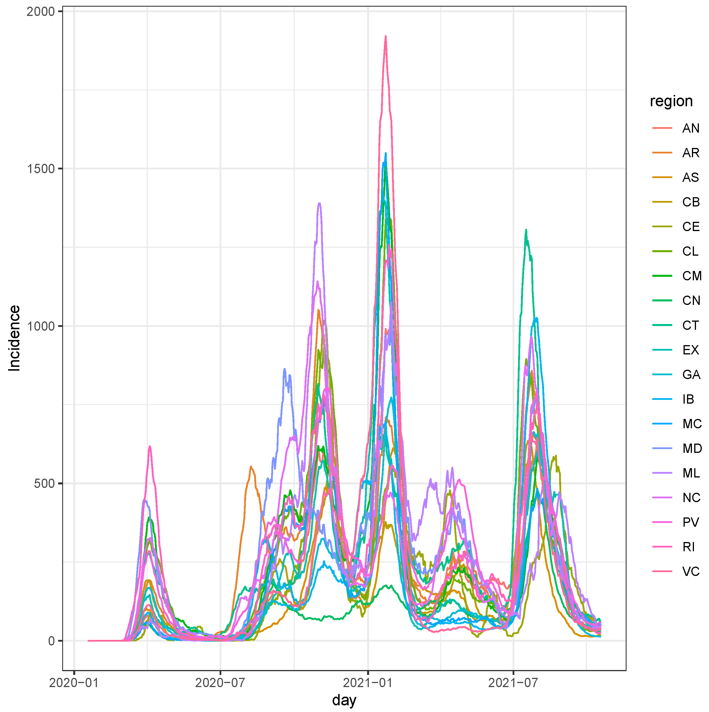
In this section, we apply the above model to estimate the evolution of COVID-19 in Spanish regions. Results here refer to data available up to the 18 October 2021.

3.1. Data

The data is from the Instituto Carlos III de Madrid in Madrid at https://cnecovid.isciii.es/covid19/resources/casos_diag_ccaadecl.csv (accessed on the 25 October 2021). These are the most reliable data for Spain available at the moment. From the database, we used the total number of reported cases from different types of tests. Such a number is not updated regularly, especially at the beginning of the spread, so observed counts for the last days may be outdated. Hence, we considered the cumulative incidence over 14 days, which leads to more reliable information about the dynamic of the pandemic. That is for the number of residents in region s, $Po{p}_s$, the sum over 14 days leading to $Y_{ts}\times Po{p}_s/\mathrm{100,000}$ compensates all under sampling effects mentioned above.

Figure 1 reports the observed incidence, $y_{ts}$ over all regions and all available periods. Five waves are present in the observed period. The period starts the 18 January 2020 till the 18 October 2021 for a total of $T=640$ days by $S=19$ regions. Starting the 18 January 2020, at the day of the first reported case in Spain (the 29 March), it is more justified from the modelling approach as, in theory, the domain of the Poisson process of infections extends to even before when the first case showed up in China. In practice, the variability in the number of observations ($T\times S$), from the 18 January 2020 until the day of the first reported case in Spain, does not practically affect the estimations.

ISO standards (https://en.wikipedia.org/wiki/ISO_3166-2:ES (accessed on the 25 October 2021)) represent the Spanish regions in all figures and tables.

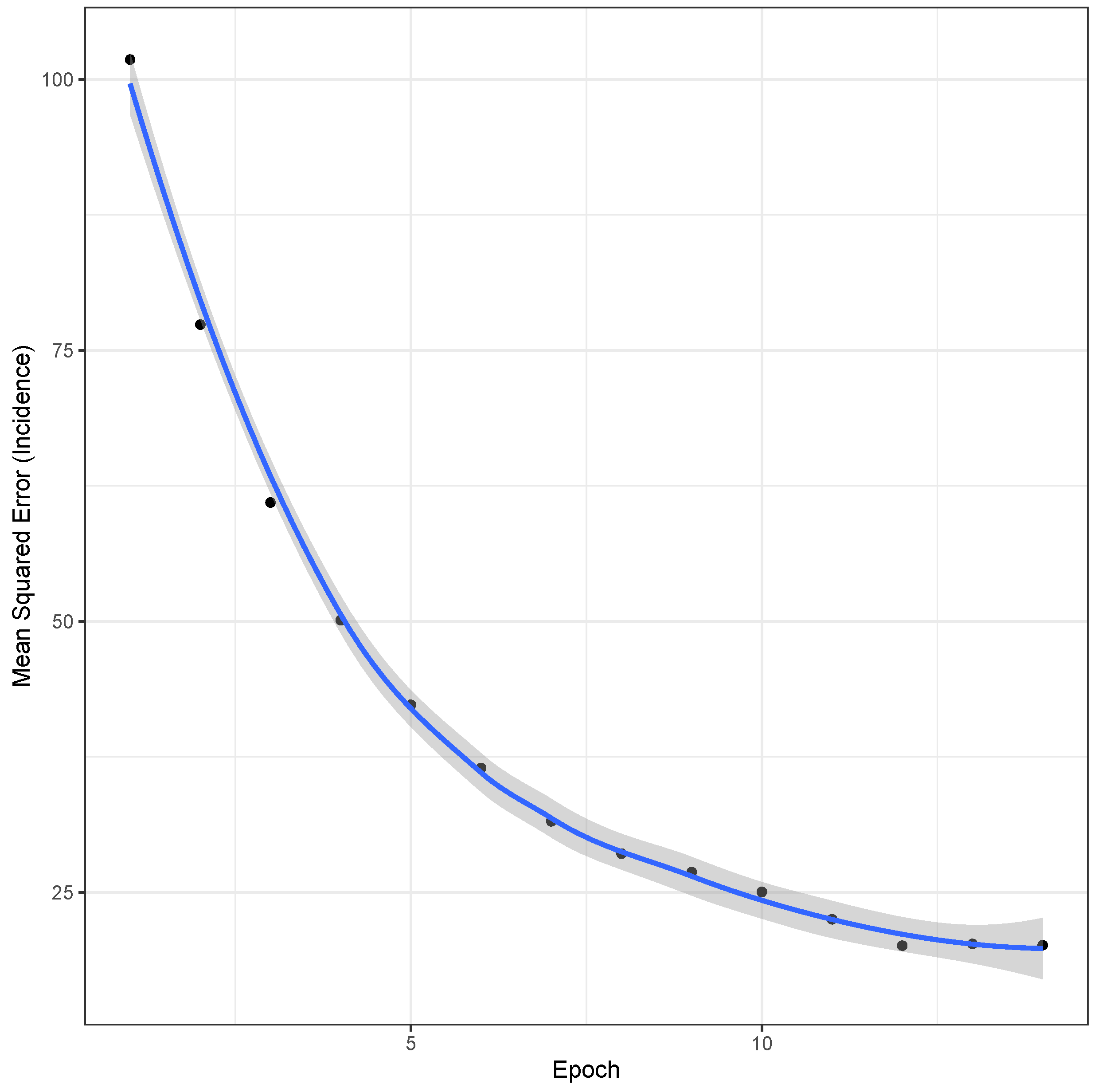
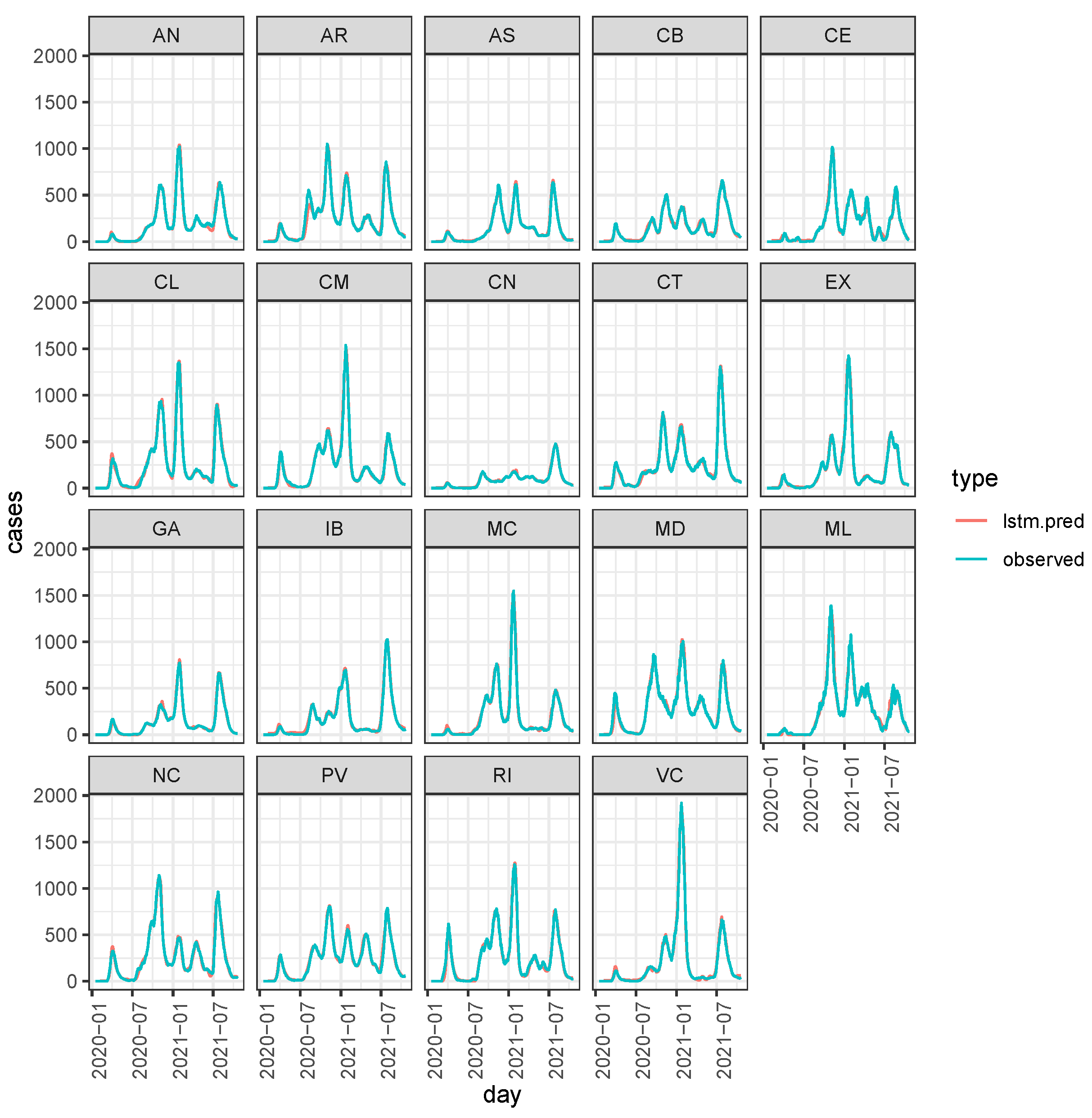
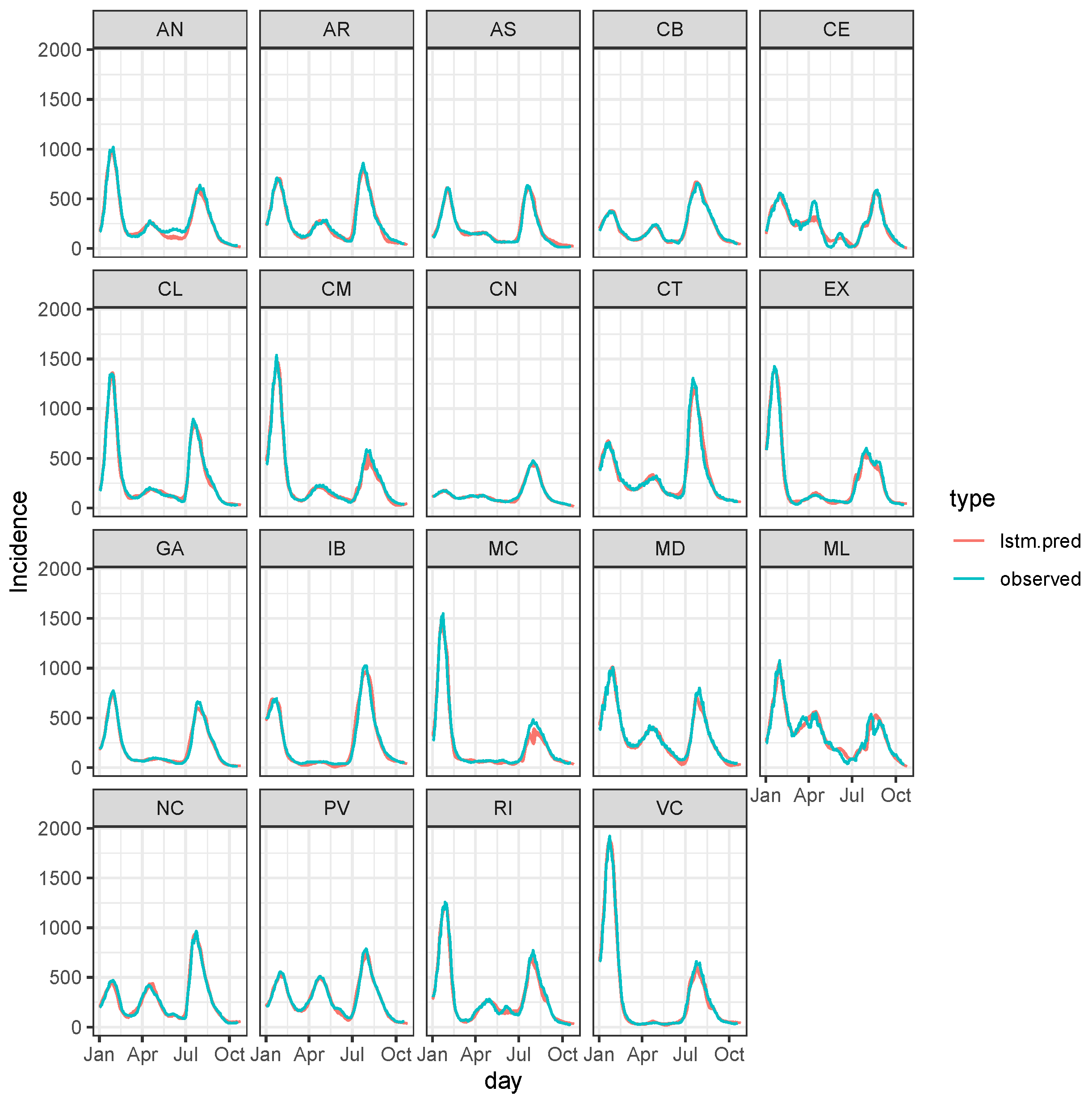
3.2. LSTM Interpolation

The presence of noisy counts reported in Figure 1 justifies the need for using robust models to describe the data. The bidirectional LSTM model looks back (and forward), and the input is a batch of $k=14$ days: the usual two weeks for an asymptomatic case to become symptomatic and show up in the database as a case. At each time t, for the backward direction, the process filtration ${\mathcal{F}}_{\bigsqcup -\infty }$ refers to the history up to two weeks before. In contrast, the forward part estimates the evolution of the two weeks ahead.

The DL model has two stacked layers of neurons: 64 LSTM layers (for each direction), and the second is a layer of $19\times 7$ (i.e., $d=7$) all connected linear neurons. The model capability is of around 52 thousand weights (nodes are all connected). Most will be zero as the data are not informative enough to update all original zero weights.

Such architecture models the following:

• sequence evolution, that is, $Y_{ts}|Y_{t^{\prime }s}$ for all $t^{\prime }\ne t$;
• between-sequence evolution that is $Y_{ts}|Y_{t^{\prime }{s}^{\prime }}$ for all $t^{\prime }\ne t$, $s^{\prime }\ne s$.

It means that, for instance, the number of cases in Madrid could be affected by past incidences in other regions, and it will affect future cases (in sequence evolution) in all other areas (between-sequence evolution). Thus, the between-sequence evolution models are contagious at the area level instead of at individual levels like the SEIR model. Modelling COVID-19 in the above way is the main contribution to the current literature on modelling the COVID-19 evolution already mentioned above.

The iterative fitting process of model weights consists of 17 steps (epochs), and the training sample at each stage has 21 random sequences ($k+d=21$ subsequent rows of the original data matrix $\mathcal{D}$ of size $T\times S$). Thus, the initial point of each sequence is random, and training sequences may overlap.

All nodes in the network are linear in their arguments. Therefore, weights are estimated to minimize the mean absolute error between the obtained counts from the final nodes and observed ones.

For the 17 steps, Figure A1 reports the estimation error, which decreases at a low plateau along with steps meaning that the network learned from the available sample. A lack of overfitting is deduced by looking at Figure A1 and also at the behaviour of the predictions on the test set (Figure A5). This statement is appropriate as the number of parameters is larger than the observed counts. This result is also related to model capability, which differs from the model dimension typical in usual regression analysis (without shrinkage methods). The standard regression model imposes to estimate all parameters from the data, while this is not necessary here. Thus, only nodes with non zero weights account for relevant information in the data, and the over-fitting is somehow limited (the training error is bounded away from zero).

Figure 2 shows the distribution of differences ${\widehat{y}}_{ts}-y_{ts}$ conditionally to region and the number of days ahead in the prediction, the delay d.

The variance of each distribution in Figure 2, $Var\left({\widehat{y}}_{ts}\right)$, is used as the prior variance (6). The general error is around 0, and predicting with more days ahead leads to greater errors. However, this is not constant over regions, and there are regions whose dynamics are more difficult to predict than others. This is again corroborated in Figure 3, where we can see that observed $y_{ts}$ and predicted ${\widehat{y}}_{ts}$ are barely indistinguishable.

It seems that the LSTM expects a decrease of cases during October 2021 in all regions, but that decrease reached a plateau, indicating that COVID-19 will not disappear in Spain. Looking at the prediction over the whole period (Figure A2 in Appendix A), predicted and observed are barely distinguishable, suggesting that the LSTM expert is generally reliable for eliciting prior (4).

Even if the observed sequences are noisy, the point is that such noise is common in many regions, and paradoxically it turns out to be “regular noise”. That is, the network can detect the effect of under-reporting counts. However, like those mentioned in the introduction, simple models may not account for this unless very informative experts were available for assessing interactions among the 19 series of counts.

The LSTM “expert” indicates that the incidence decreasing is slowing down in many regions. But, of course, we have no clue how much is probable in the above statements, and the following Section 3.3 addresses it. The additional problem in using the output of a DL model directly is that it is challenging to understand why that decrease/increases in the number of cases, which casts doubt on the direct use of such an output as a final prediction. However, why should a model that did well in the past failures in the future? Is this due to overfitting? The subsequent Bayesian analysis addresses them by assigning probabilities to the two statements: (1) how well did it do in the past? And (2) how much do we trust the predicted future? However, specifically to the overfitting problem, we already estimated the prediction errors on d days. Given that the number of time points is large, then $Var\left({\widehat{y}}_{ts}\right)$ estimated from Figure 2 is a reliable estimation of the model’s goodness: the model fits well for the days that were not into the k past days used to predict it.

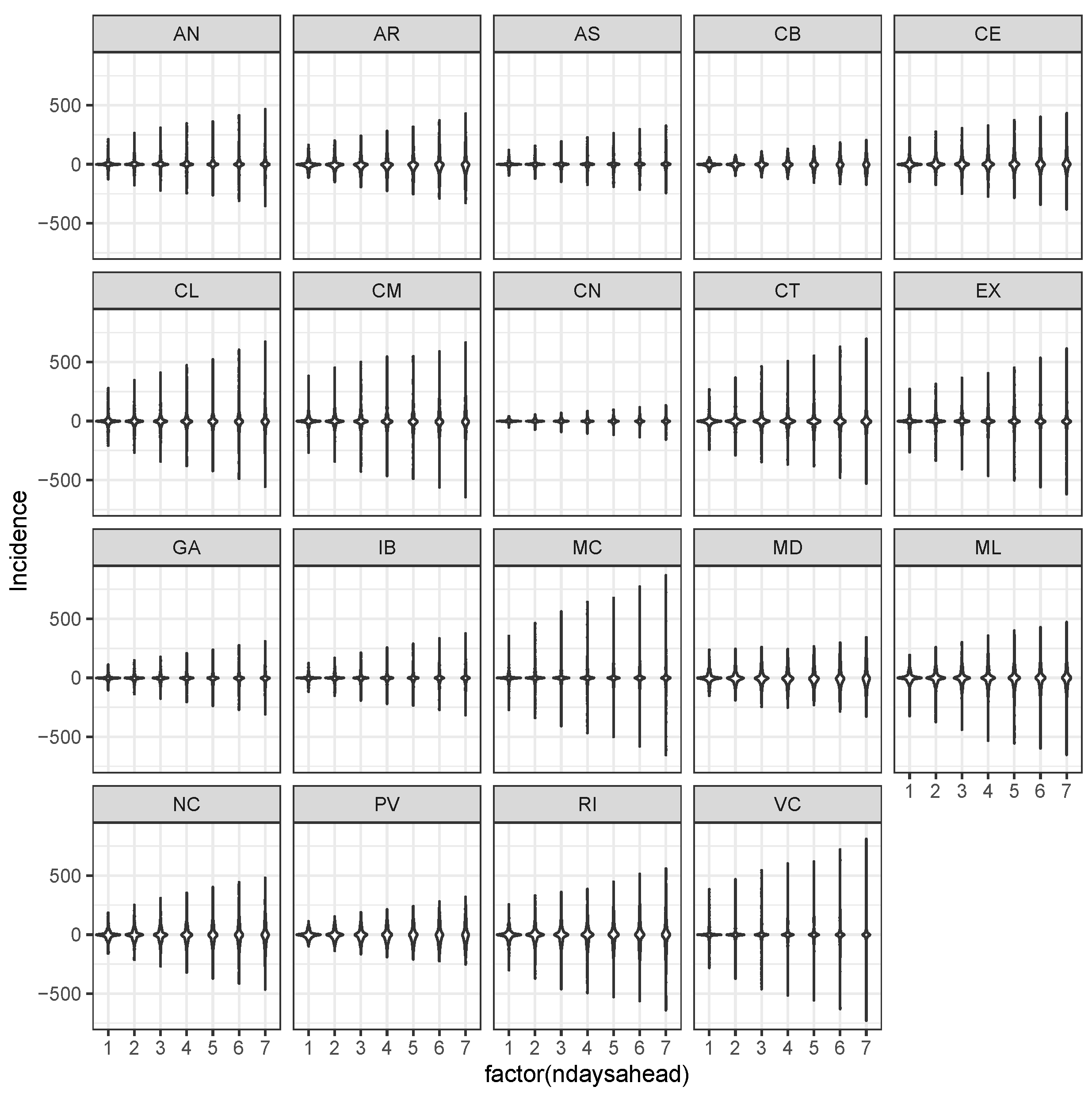
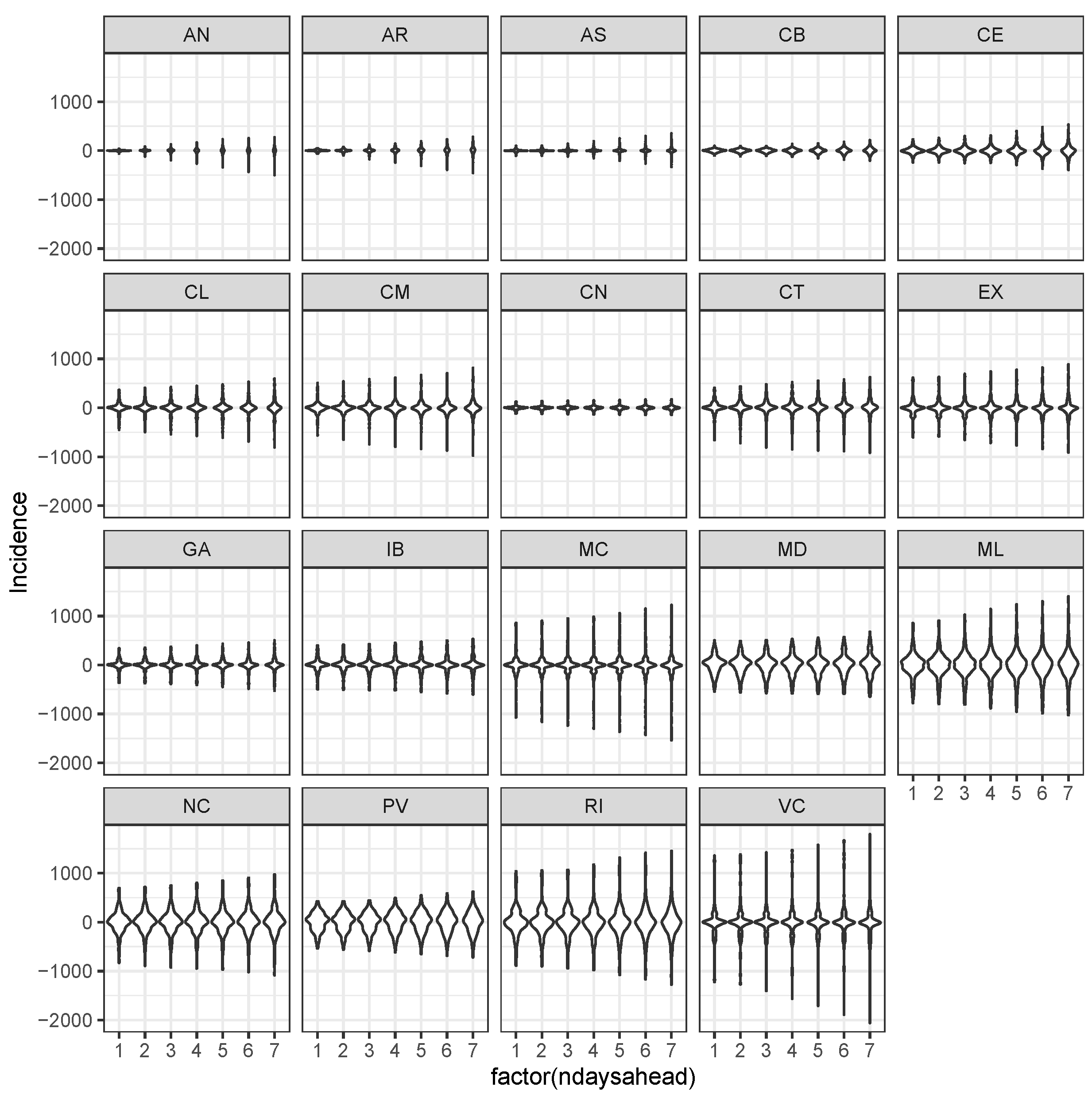
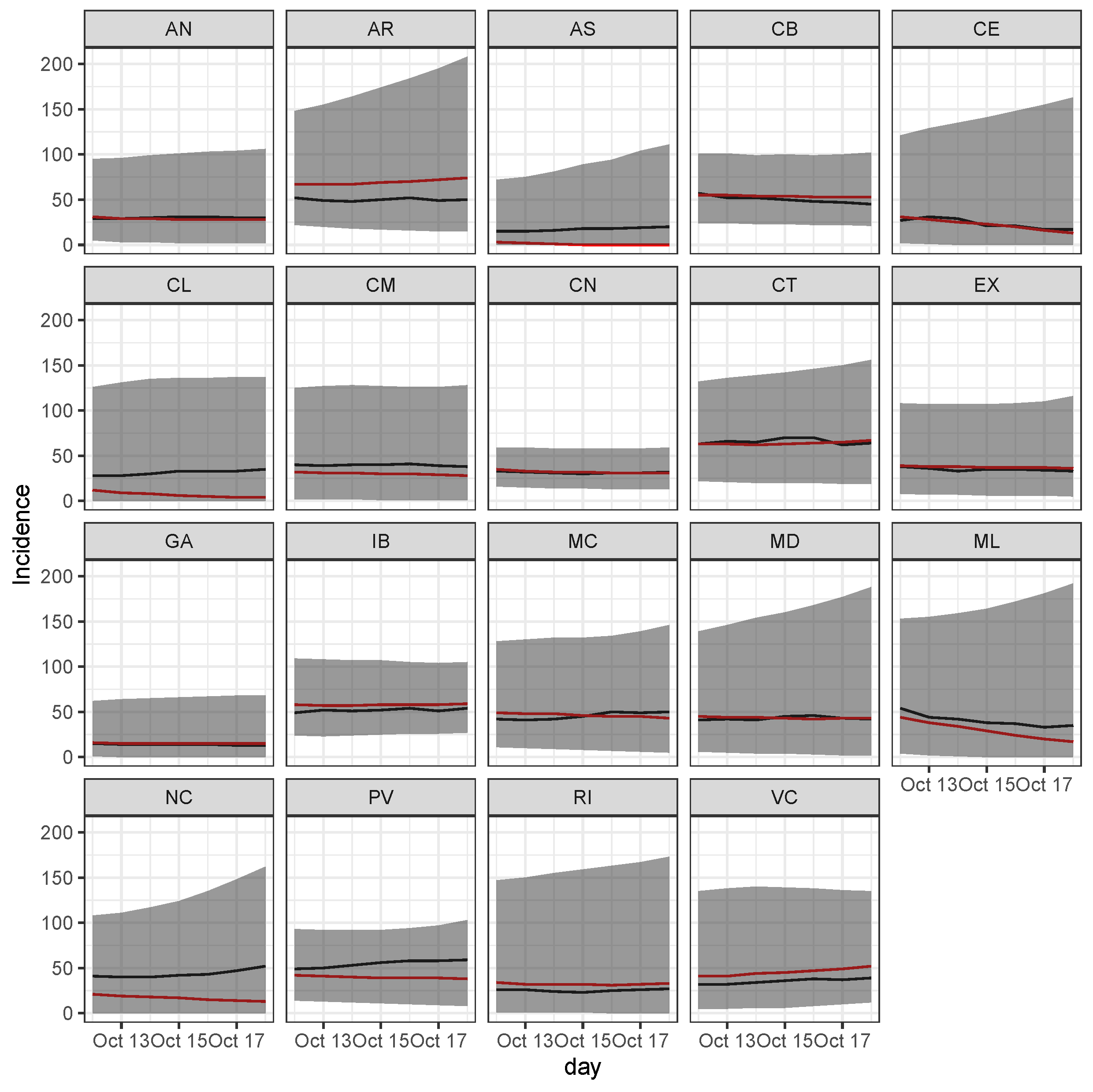
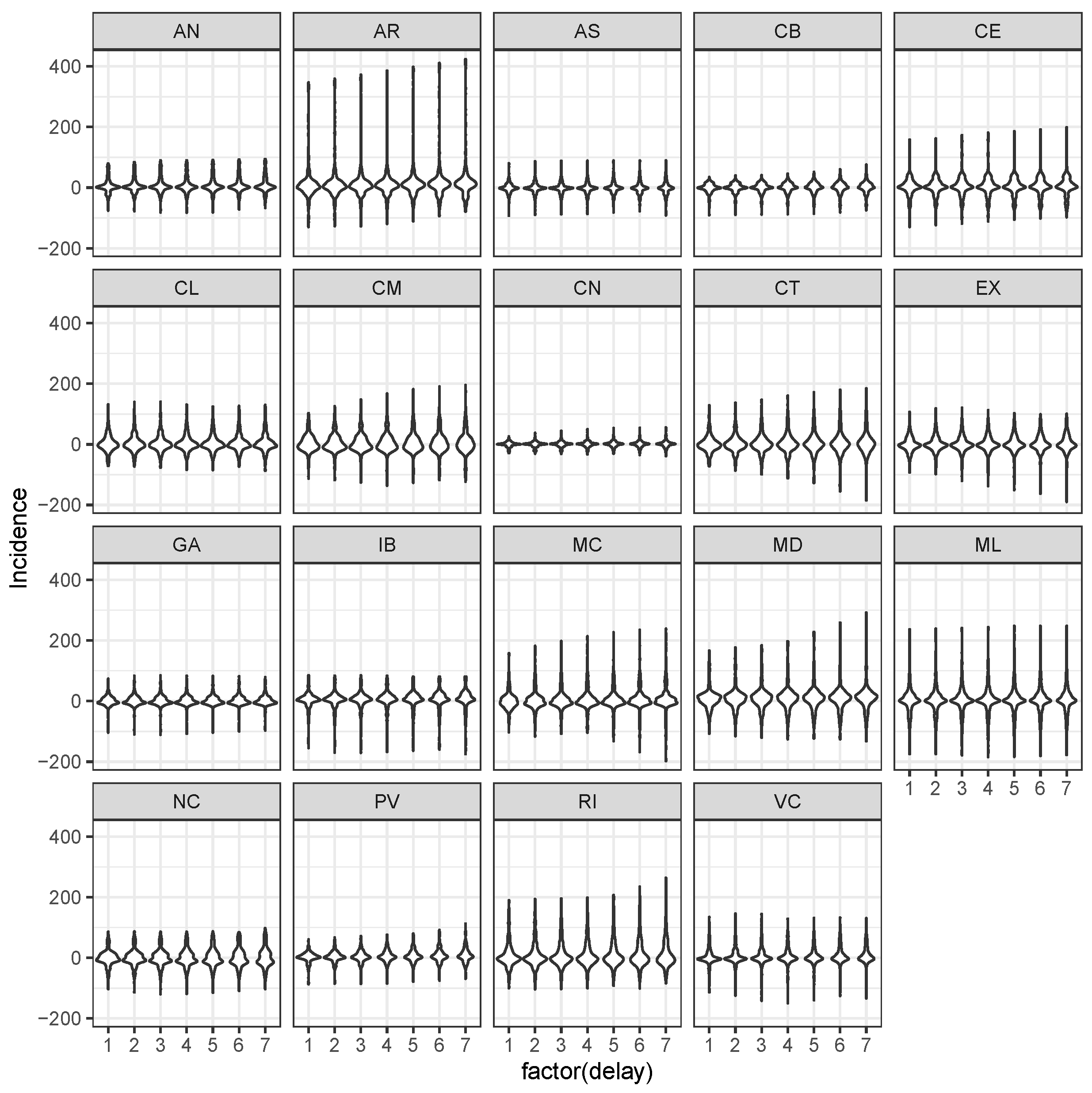
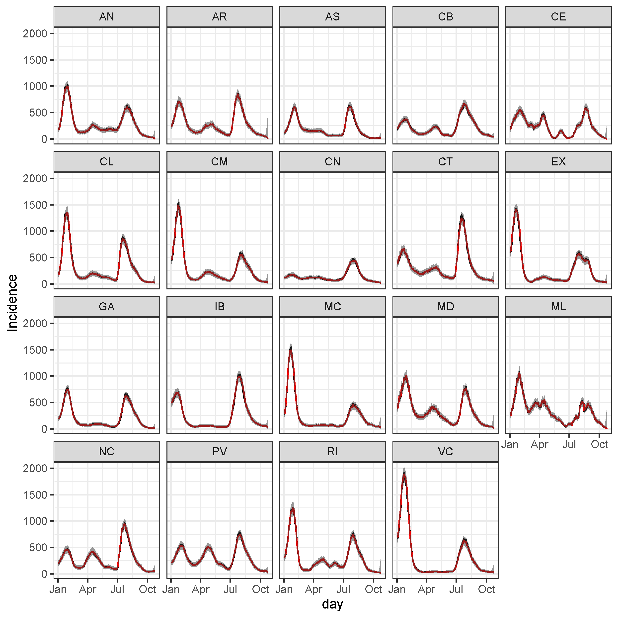
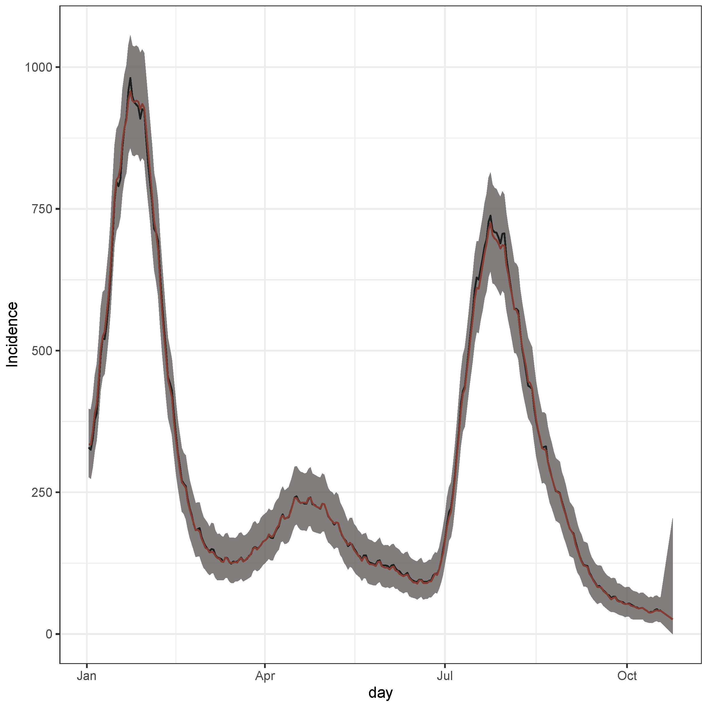
3.3. Bayesian Predictive Analysis and Goodness of Fit Assessment

Results shown in Figure 3 and the above LSTM model do not convey a proper evaluation of the uncertainty around the estimation of days ahead evolution. For this purpose, we calculate the posterior predictive distribution of $Y_{ts}$ according to (7) and (8).

The result is the prediction along with its uncertainty, which is the estimation of (1). Figure 4 we report the observed and predicted (with the median) counts along with 99% equal tail credible intervals (CI).

From Figure 4 we can see that accounting for the uncertainty, the observed values are compatible with 99% CI. Moreover, this uncertainty increases for unobserved days, the last seven days, namely from the 12 October till the 18 October.

The overall prediction for Spain is the weighted average over regional predictions, where weights are proportional to the resident region’s population. This is shown in Figure 5.

From Figure 5 we can appreciate a general decrease of the incidence, which should be below 100 cases per 100,000 residents for the next week.

To further validate the model, the LSTM expert was trained up to the last observed seven days, such that their prediction comes from (8).

Figure A5 shows that the observed incidence is almost compatible, taking into account the uncertainty provided by the Bayesian model. The CI uncertainty is ample for two reasons: past jumps in counting the number of cases (e.g., changes in collecting protocol) and the nominal CI level, 99%. Thus, considering lower nominal values (e.g., 95% or 90%) narrows CI at the cost of less coverage.

Using the median of the Negative Binomial predictive posterior distribution, (1) we have average marginal error (per day and region) over the test set of just six cases over 100,000 people with a standard deviation of 12 cases. Such a result indicates that the final prediction is very accurate over this test set.

Figure A5 further shows that the observed incidence in some regions is forecast with more precision than others.

Table A1. Predicted incidence ${\widehat{y}}_{ts}$ with their 99% CI and observed daily incidence over last observed week (12th till October 18th). These observations are out of the training sample. The first day is one day ahead prediction, and the last is seven days ahead prediction. These numbers appear in Figure A5.

		Number of Days Ahead Predictions
Region	Variable	1	2	3	4	5	6	7
AN	inf (0.5%)	6	5	4	4	4	3	2
AN	obs.	29	29	30	31	31	30	30
AN	pred (50%)	41	40	40	41	41	40	39
AN	sup (99.5%)	128	132	137	142	147	153	162
AR	inf (0.5%)	0	0	0	0	0	0	0
AR	obs.	52	49	48	50	52	49	50
AR	pred (50%)	41	38	37	36	35	34	34
AR	sup (99.5%)	385	394	404	415	426	438	449
AS	inf (0.5%)	0	0	0	0	0	0	0
AS	obs.	15	15	16	18	18	19	20
AS	pred (50%)	2	3	4	4	4	5	4
AS	sup (99.5%)	195	197	204	213	222	230	240
CB	inf (0.5%)	11	9	7	5	4	3	2
CB	obs.	57	52	52	50	48	47	45
CB	pred (50%)	43	41	41	39	39	38	37
CB	sup (99.5%)	104	110	117	124	132	140	150
CE	inf (0.5%)	0	0	0	0	0	0	0
CE	obs.	27	31	29	21	21	17	17
CE	pred (50%)	30	25	23	22	20	18	16
CE	sup (99.5%)	192	200	207	215	222	230	239
CL	inf (0.5%)	0	0	0	0	0	0	0
CL	obs.	28	28	30	33	33	33	35
CL	pred (50%)	31	27	26	26	25	24	24
CL	sup (99.5%)	181	199	215	234	255	280	307
CM	inf (0.5%)	0	0	0	0	0	0	0
CM	obs.	40	39	40	40	41	39	38
CM	pred (50%)	31	26	23	22	20	18	17
CM	sup (99.5%)	231	266	298	328	359	393	430
CN	inf (0.5%)	9	8	8	8	7	7	7
CN	obs.	33	32	31	30	31	31	32
CN	pred (50%)	35	34	34	34	33	33	33
CN	sup (99.5%)	84	84	84	85	85	86	88
CT	inf (0.5%)	9	8	7	6	5	4	4
CT	obs.	63	66	65	70	70	62	64
CT	pred (50%)	79	78	78	78	78	78	77
CT	sup (99.5%)	269	280	294	308	323	338	354
EX	inf (0.5%)	0	0	0	0	0	0	0
EX	obs.	38	36	33	35	35	34	33
EX	pred (50%)	31	28	26	22	19	17	15
EX	sup (99.5%)	223	258	298	337	377	416	454
GA	inf (0.5%)	0	0	0	0	0	0	0
GA	obs.	15	14	14	14	14	13	13
GA	pred (50%)	13	12	13	14	13	13	12
GA	sup (99.5%)	101	101	105	110	117	125	136
IB	inf (0.5%)	6	6	5	5	4	3	3
IB	obs.	49	52	51	52	54	51	54
IB	pred (50%)	54	56	56	57	58	58	59
IB	sup (99.5%)	192	199	207	217	230	244	259
MC	inf (0.5%)	0	0	0	0	0	0	0
MC	obs.	42	41	42	45	50	49	50
MC	pred (50%)	15	9	7	4	2	1	0
MC	sup (99.5%)	324	379	423	473	527	581	638
MD	inf (0.5%)	0	0	0	0	0	0	0
MD	obs.	41	42	41	45	46	43	42
MD	pred (50%)	23	22	24	25	25	26	26
MD	sup (99.5%)	186	206	225	243	262	282	303
ML	inf (0.5%)	5	3	2	1	0	0	0
ML	obs.	54	44	42	38	37	33	35
ML	pred (50%)	57	51	47	43	40	37	33
ML	sup (99.5%)	211	214	218	224	232	242	255
NC	inf (0.5%)	3	2	2	1	1	1	0
NC	obs.	41	40	40	42	43	47	52
NC	pred (50%)	36	35	37	37	38	37	38
NC	sup (99.5%)	138	144	155	167	182	200	219
PV	inf (0.5%)	1	2	2	2	2	2	2
PV	obs.	49	50	53	56	58	58	59
PV	pred (50%)	49	50	50	52	53	52	53
PV	sup (99.5%)	252	239	236	236	238	242	247
RI	inf (0.5%)	0	0	0	0	0	0	0
RI	obs.	26	26	24	23	25	26	27
RI	pred (50%)	19	14	13	11	9	7	5
RI	sup (99.5%)	232	244	261	281	305	335	372
VC	inf (0.5%)	0	0	0	0	0	0	0
VC	obs.	32	32	34	36	38	37	39
VC	pred (50%)	42	38	38	37	37	37	36
VC	sup (99.5%)	251	278	307	336	366	395	425

reports the values in Figure A5.

To formally check model Goodness of Fit (GOF), we can again look at Figure A5 and see that all prediction intervals for all regions contain the future observed incidence values. The observed proportion (100%) is near the nominal 99% of probability for the reported credible intervals. However, the observed values in Figure A5, are not used to fit the model, and checking with them agrees with [15] and [16] which warns about the double use of the data: first to fit the model and then to assess its GOF.

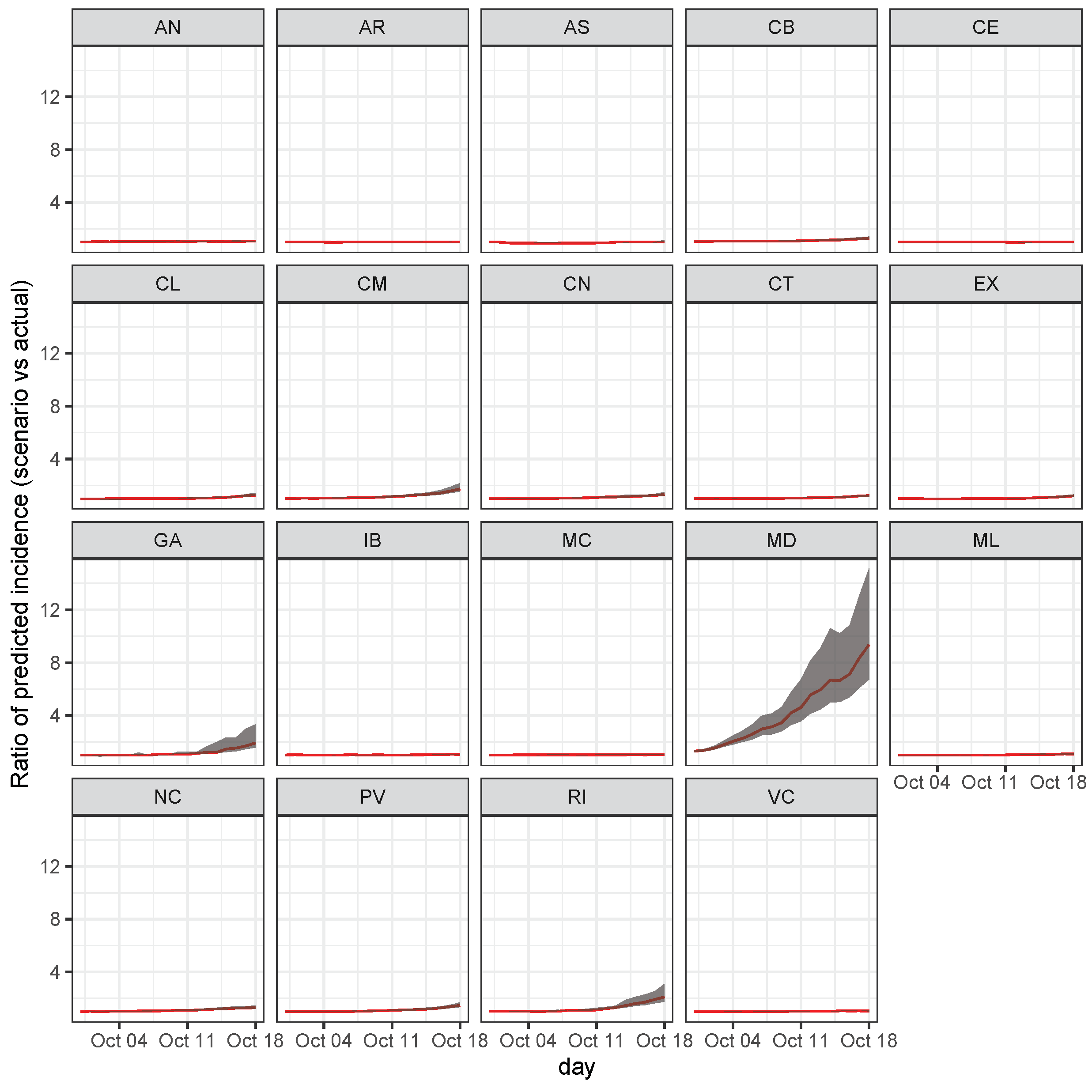
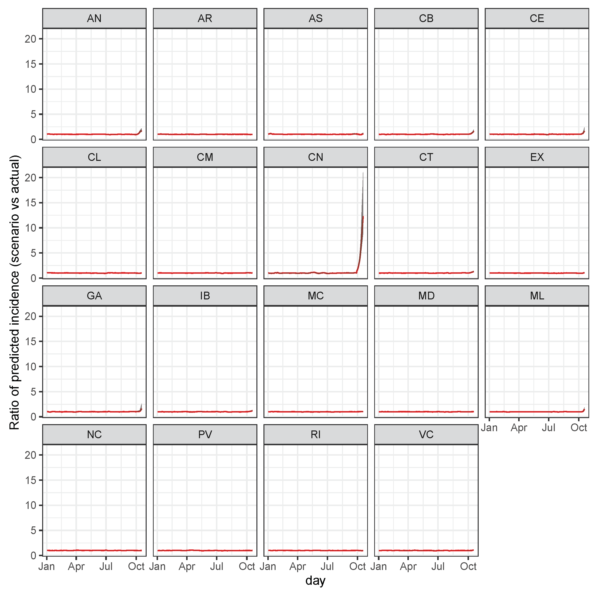
3.4. Impact Scenarios

This section is devoted to analyzing the impact of hypothetical scenarios and thus illustrates how public policymakers can eventually use this model. This section also has a twofold purpose: first, to analyze the impact of plausible scenarios in making predictions and, secondly, to interpret the overall model given that the LSTM projections lack a straightforward interpretation. DL models are black boxes. For instance, a perturbation in a region and the impact on other areas can shed light on the spatial relation between areas that the LSTM learned from the data.

3.4.1. Scenario 1: The Case of Increase in Madrid

Suppose that during the last 20 days up to the previously observed day, the number of cases in the Madrid region was artificially increased by 10% every day from the day before (i.e., the reproduction rate is 1.1). What should be the impact on other areas?

Figure A6 reports the ratio between the predicted incidence for the scenario and current estimations.

This scenario induces a sure increment of cases in the rest of the country, and in most regions, this increment is significant even considering the prediction uncertainty.

3.4.2. Scenario 2: Cases Increase in the Canary Islands

Suppose that the same number of cases as in scenario 1 occur in the Canary Islands, with a smaller population and a more dispersed one than the Madrid region. Figure A7 reports the impact on all of Spain.

Contrary to the previous scenario, an increase in the incidence in the Canary Islands does not induce a general solid increment of the incidence in other regions. Such an effect could be because, being isolated, the dynamic of the Canary Islands is not so related to the COVID-19 dynamics in the rest of Spain. That’s what the model learned from the data.

4. Discussion

The proposed analysis can extend to temporal and spatial effects by using other DL architectures, such as Convolutional Neural Networks (CNN). CNN is a specific class of DL models suitable for analyzing structured samples as images [17] which can be generalized to time and spatial dimension. The spatial dimension is here not imposed into the model because of the reason explained in Section 1, as it is not clear how to define the surrounding areas relevant for describing the evolution of COVID-19. Experience has suggested that COVID-19 appeared in different regions of the world almost at the same time. The idea here is that capturing relations among the dynamics of counts of other areas improves over estimating relations among counts.

Other DL architectures are even more popular than the LSTM for modelling counts. In particular, we recall Echo networks [18] and self-attention networks [19]. Comparing the proposed approach with these architectures would be an interesting exercise that is out of the scope of this paper. However, the interest in the DL architecture matters only at the level of the prior distribution and not the likelihood. The proposed priors can be more or less informative depending on their success in estimating the test set, and the prior variance (6) accounts for it.

To compare the proposed approach with others, we consider Vector Autoregressive (VAR) linear models [20] for modelling these data. This model jointly considers all series, and thus the spatial correlation (a linear dynamic) for all regions is accounted into one model. A joint model is necessary more to gather evidence from one region to others and to make a scenario analysis like that in Section 3.4. A VAR model of order 1 is considered and it just regresses the vector of responses $log(1+Y_{(2:t)(1:S)}$ over past values up to $t-1$: $log(1+Y_{(1:t-1)(1:S)}$, where the subscript $(i:j)$ indicates that for any pair of integers $(i,j)$, with $i\le j$ denote the observations from the ith to the jth, inclusive. Coefficients estimators are the Maximum Likelihood ones. The estimated model would replace the LSTM model in our proposal. However, if the prediction errors from the VAR model would be larger than the LSTM, the final predictions, even under the Poisson-Gamma model in Section 2.2 would also have large uncertainty and bias. Therefore, it is important to compare the errors in Figure 2 with that of the VAR model reported in Figure A3. In this case, we can see that errors with the VAR have around five orders of magnitude compared to the proposed LSTM. A possible explanation is that the spatial and temporal relationships among regional incidences are much more complex than those assumed in the VAR model.

Another model for comparison purposes would be a multivariate Dynamic Linear Model (DLM) [21]. The number of involved parameters for these models grows with S, and thus, the posterior mode for these parameters is difficult to estimate. Therefore, this implies modelling each region independently, preventing it from being used in scenario analysis (Section 3.4). Concretely, we used a seventh order polynomial DLM. The latent state on the mean has dimension seven. Similarly to the VAR model, the posited DLM considers advance predictions of seven days, the seven days ahead evolutions of the state variable Y. Again, comparing the errors in Figure 2 with that of the DLM model reported in Figure A4, we can see that the latter are much larger than that with LSTM. Thus, using a seventh order polynomial DLM, the temporal dynamic at each region is much more complex than that assumed by the posed DLM.

5. Conclusions

The proposed modelling approach is general in its essential lines (DL model to elicit priors), and it can be applied to analyze spatiotemporal models for counts. It can incorporate other definitions of regions, such as a province or hospital areas or even point data from geo-localization of cases. It could include other covariates on estimating the evolution of COVID-19, such as meteorological data if they were relevant or in the presence of social restriction measures. The GitHub code makes this kind of generalization of the analysis here proposed relatively easy. The model assumes that all evolution processes can be learned from the observed counts and not from other sources of information as, for instance, social mobility or the vaccination campaign.

The proposed model allows us to account for the complexity of the evolution of COVID-19 in Spain by summarizing it in a complicated model structure represented by the bidirectional LSTM network whose output serves as an input for a Bayesian Poisson-Gamma model. The latter finally accounts for the randomness and proper conditional inference of the pandemic evolution given the collected counts.

The important message here is that relying on a single approach for estimating the evolution of COVID-19 (i.e., only machine learning or only parametric Bayes) is not optimal. Still, the combination of different methods would be more profitable. On the contrary, the drawback of this hybrid approach is that it becomes difficult to assess the overall theoretical reliability. For instance, we know very well that the Poisson-Gamma model leads to estimates close to the true one (in mean squared error) when the prior precision is not too high. However, we don’t have explicitly theoretical results on the consistency of LSTM models, although there exists other successful applications of LSTM [22]. Furthermore, there is no theoretical consistency in the proposed hybrid models.

In contrast, we here face a concrete (not theoretical) problem of predicting and forecasting the evolution of COVID-19. Other theories may arrive in the future to support or disprove the proposed two-stage approach.

References

1. Li, M.Y.; Muldowney, J.S. Global stability for the SEIR model in epidemiology. Math. Biosci. 1995, 125, 155–164. [Google Scholar] [CrossRef]
2. Agosto, A.; Cavaliere, G.; Kristensen, D.; Rahbek, A. Modeling corporate defaults: Poisson autoregressions with exogenous covariates (PARX). J. Empir. Financ. 2016, 38, 640–663. [Google Scholar] [CrossRef] [Green Version]
3. Agosto, A.; Giudici, P. A Poisson Autoregressive Model to Understand COVID-19 Contagion Dynamics. Risks 2020, 8, 77. [Google Scholar] [CrossRef]
4. Paul, M.; Held, L. Predictive assessment of a non-linear random effects model for multivariate time series of infectious disease counts. Stat. Med. 2011, 30, 1118–1136. [Google Scholar] [CrossRef] [PubMed]
5. Giuliani, D.; Dickson, M.M.; Espa, G.; Santi, F. Modelling and predicting the spread of Coronavirus (COVID-19) infection in NUTS-3 Italian regions. BMC Infect. Dis. 2020, 20, 700. [Google Scholar]
6. Davis, R.A.; Fokianos, K.; Holan, S.H.; Joe, H.; Livsey, J.; Lund, R.; Pipiras, V.; Ravishanker, N. Count time series: A methodological review. J. Am. Stat. Assoc. 2021, 3, 1–15. [Google Scholar] [CrossRef]
7. Schmidhuber, J. Deep learning in neural networks: An overview. Neural Netw. 2015, 61, 85–117. [Google Scholar] [CrossRef] [PubMed] [Green Version]
8. Breiman, L. Statistical modeling: The two cultures (with comments and a rejoinder by the author). Stat. Sci. 2001, 16, 199–231. [Google Scholar] [CrossRef]
9. Polson, N.G.; Sokolov, V. Deep Learning: A Bayesian Perspective. Bayesian Anal. 2017, 12, 1275–1304. [Google Scholar] [CrossRef]
10. Abadi, M.; Agarwal, A.; Barham, P.; Brevdo, E.; Chen, Z.; Citro, C.; Corrado, G.S.; Davis, A.; Dean, J.; Devin, M.; et al. TensorFlow: Large-Scale Machine Learning on Heterogeneous Systems, 2015. Software. 2015. Available online: tensorflow.org (accessed on 25 August 2021).
11. Lim, B.; Zohren, S. Time-series forecasting with deep learning: A survey. Philos. Trans. R. Soc. A 2021, 379, 20200209. [Google Scholar] [CrossRef] [PubMed]
12. Sherstinsky, A. Fundamentals of Recurrent Neural Network (RNN) and Long Short-Term Memory (LSTM) network. Phys. D Nonlinear Phenom. 2020, 404, 132306. [Google Scholar] [CrossRef] [Green Version]
13. West, M.; Harrison, J. The Dynamic Linear Model. In Bayesian Forecasting and Dynamic Models; Springer: New York, NY, USA, 1989; pp. 105–141. [Google Scholar] [CrossRef]
14. Wöllmer, M.; Eyben, F.; Graves, A.; Schuller, B.; Rigoll, G. Bidirectional LSTM networks for context-sensitive keyword detection in a cognitive virtual agent framework. Cogn. Comput. 2010, 2, 180–190. [Google Scholar] [CrossRef] [Green Version]
15. Conn, P.B.; Johnson, D.S.; Williams, P.J.; Melin, S.R.; Hooten, M.B. A guide to Bayesian model checking for ecologists. Ecol. Monogr. 2018, 88, 526–542. [Google Scholar] [CrossRef]
16. Bayarri, M.; Castellanos, M. Bayesian checking of the second levels of hierarchical models. Stat. Sci. 2007, 22, 322–343. [Google Scholar]
17. Rawat, W.; Wang, Z. Deep Convolutional Neural Networks for Image Classification: A Comprehensive Review. Neural Comput. 2017, 29, 2352–2449. [Google Scholar] [CrossRef] [PubMed]
18. Jaeger, H. The “Echo State” Approach to Analysing and Training Recurrent Neural Networks-with an Erratum Note; GMD Technical Report; German National Research Center for Information Technology: Bonn, Germany, 2001; Volume 148, p. 13. [Google Scholar]
19. Wu, Y.; Ma, Y.; Liu, J.; Du, J.; Xing, L. Self-attention convolutional neural network for improved MR image reconstruction. Inf. Sci. 2019, 490, 317–328. [Google Scholar] [CrossRef] [PubMed] [Green Version]
20. Hamilton, J.D. Time Series Analysis; Princeton University Press: Princeton, NJ, USA, 2020. [Google Scholar]
21. Campagnoli, P.; Petrone, S.; Petris, G. Dynamic Linear Models; Springer: New York, NY, USA, 2009. [Google Scholar]
22. Karpatne, A.; Atluri, G.; Faghmous, J.H.; Steinbach, M.; Banerjee, A.; Ganguly, A.; Shekhar, S.; Samatova, N.; Kumar, V. Theory-guided data science: A new paradigm for scientific discovery from data. IEEE Trans. Knowl. Data Eng. 2017, 29, 2318–2331. [Google Scholar] [CrossRef]
Figure 1. Observed cumulative incidence at 14 days for the 19 Spanish regions. The period starts 18 January 2020 and ends on 18th October 2021 for a total number of T = 640 days by S = 19 regions.
Mathematics 09 02921 g001
Figure 2. Violin plots of distributions of differences y ^ t s y t s conditionally to the region and the number of days ahead in the prediction, namely the delay d. The variance of the LSTM used for the Poisson mean elicitation is just the average of the squared differences y ^ t s y t s . These increase as there is more uncertainty in predicting with delay d = 7 than d = 1 .
Mathematics 09 02921 g002
Figure 3. Predicted y ^ t s and observed daily incidence over 2021 only.
Mathematics 09 02921 g003
Figure 4. Daily incidence for year 2021. Posterior predicted distribution summarized by the median (red) and 99% credible intervals (shaded grey area) for observed days (black) This is the estimation of (1) for observed and future predictions starting from d = 1 day ahead up to d = 7 days ahead, namely from 12 October till 18 October.
Mathematics 09 02921 g004
Figure 5. Daily incidence for the year 2021 for overall Spain. Posterior predicted distribution summarized by the median (red) and 99% credible intervals (shaded grey area) for observed days (black) This is the estimation of (1) for observed and future predictions starting from d = 1 day ahead up to d = 7 days ahead, namely from 12 October till 18 October.
Mathematics 09 02921 g005
Publisher’s Note: MDPI stays neutral with regard to jurisdictional claims in published maps and institutional affiliations.