Adaptive Active Disturbance Rejection Control of Solar Tracking Systems with Partially Known Model

Abstract

In this article, the trajectory tracking control of a solar tracking system is tackled by means of an adaptive active disturbance rejection control scheme. The state and disturbance estimation system is based on the combination of a time varying identification system and an adaptive observer. The stability and robustness of the controller is mathematically tested by means of the second method of Lyapunov, and its effectiveness is experimentally tested in a robotic test bed, achieving both lower energy consumption and better tracking results with respect to a PID-based controller.

1. Introduction

The tendency of using alternative energy sources has led to the solution of problems concerning a wide variety of collecting technologies, storage and management systems. In the case of solar energy, the increased efficiency of the collected energy has a close relation with the capacity to manipulate the collecting device (photovoltaic module, concentrating lens, etc.) such that the light incidence is normal to a specific area of interest (tilt angle control). The last aspect is especially important in Fresnel-lens-based concentration systems [1,2,3].

The aim to increase the benefits of energy collecting systems has led to the development of solar trackers [4,5], the efficiency of which can be improved through the use of optimal design technologies [6,7,8,9] and concurrent engineering tools [10] as well as highly accurate positioning control systems such as solar sensors [11,12,13,14,15].

The accuracy and energy consumption in the positioning policy are considered to be among the main aspects of the performance of a solar tracker. Both problems are directly related to the nature of the mechanism of the tracker, which can have uncertain dynamics or nonlinearities, and the operation may be affected by external disturbance elements such as wind disturbances, which can produce tracking errors, or high energy compensation actions reducing the energetic efficiency of the controller. Addressing both features concurrently demands robustness and an energy management adaptation.

Several control approaches are reported in the literature, and some comprehensive studies and reviews provide further information and specific features regarding existing control studies and implementations [16,17,18,19], in which the application may lead to specific precision demands (see [20]). Among recent studies, in [21], a comprehensive practical classification of active solar tracking systems is presented, focusing on the importance of the control law and the sensing technology used to achieve appropriate results in solar concentration tasks. In this sense, proportional integral derivative-based control (PID) is the most popular closed-loop strategy in active solar tracking systems (see [22,23]). This scheme is suitable for solar trackers that include a gear train transmission with a high gear ratio [24]. The strategy has a wide variety of tuning strategies, including optimal gain selection, that make this scheme the natural choice for practitioners [25].

Due to the high-gain nature of PID control, diverse tuning schemes to avoid overshooting effects are used. On one hand, some schemes based on set points or the internal model control principle have been developed [26,27]. Although these approaches are a precise alternative, some tests and several criteria are necessary to obtain the best results with the approach. In contrast, some adaptive variations of PID have been developed to ease the drawbacks of high gain by means of time-varying gain dynamics [28,29,30,31]. In [32], an adaptive gain PID controller is implemented for dual-axis sun tracker applications. The gains are normalized in terms of the tracking error, improving upon the classic PID control. However, most of the reported schemes lack time derivative measurements, which may affect the final result by using computationally costly platforms (for instance, matlab) or dirty derivative-based computation with high computational and energetic costs and possible measurement noise problems. Moreover, low gear ratio transmissions or the possible presence of nonlinearities in the mechanism or the actuator motivate robust adaptive strategies that deal with the original multivariable nonlinear tracker model.

Other control strategies include model predictive control [33,34], sliding mode control [35,36] and neural and fuzzy control [37,38,39,40]. Most of these schemes solve one of the aforementioned problems effectively, while the other important aspects are partially achieved due to the fact that optimizing strategies usually need exact information of the system and they usually work for linear models; on the other hand, robust strategies usually demand high energetic costs. This motivates the development of a control scheme that can strike a balance between robustness and adaptivity.

Active disturbance rejection control (ADRC) [41,42,43,44,45,46] represents a control paradigm in which the system can be simplified such that the main external disturbances and unknown dynamics are lumped into a generalized disturbance input to be estimated and further cancelled. This scheme provides some of the advantages of classic PID control while enhancing the performance by means of the use of extended state observers [47]. The possibility of estimating the generalized disturbance simplifies the control actions, obtaining accurate results in trajectory tracking tasks. One of the most popular approaches to active disturbance rejection is linear active disturbance rejection (LADRC) [48], which consists of the use of an extended state observer of the Luenberger type. This scheme is highly effective for the estimation of a large class of additive disturbances, and the high-gain nature of the strategy results in an easy-to-tune procedure. The high-gain nature of classic LADRC may be sensitive to noises and can increase the energy consumption in the control applications, and the compromise between robustness and low energy consumption can be improved by proposing alternative schemes that keep the estimation advantages of LADRC with some restrictions in the high-gain nature. To achieve robustness and low energy consumption, adaptive designs for the ADRC [49,50] provide accurate tracking, robustness and adaptivity, which make them suitable for solar tracking applications.

In this article, an adaptive active disturbance rejection control design is proposed to solve the problem of the trajectory tracking system in a two-axis solar tracking system. The proposed observer is based on the combination of a time-varying identification system and an adaptive observer. This combination is used for online generalized disturbance estimation, which is used in the control loop. The main contributions are listed as follows:

1.

In contrast with the disturbance estimation approach proposed in [49], in this article, the disturbance is estimated in terms of both states and an additional constant term used to compensate possible offset errors and external components that are independent of the states.

2.

The stability and robustness of the controller is mathematically tested by means of the second method of Lyapunov, and its effectiveness is experimentally tested in a robotic test bed.

3.

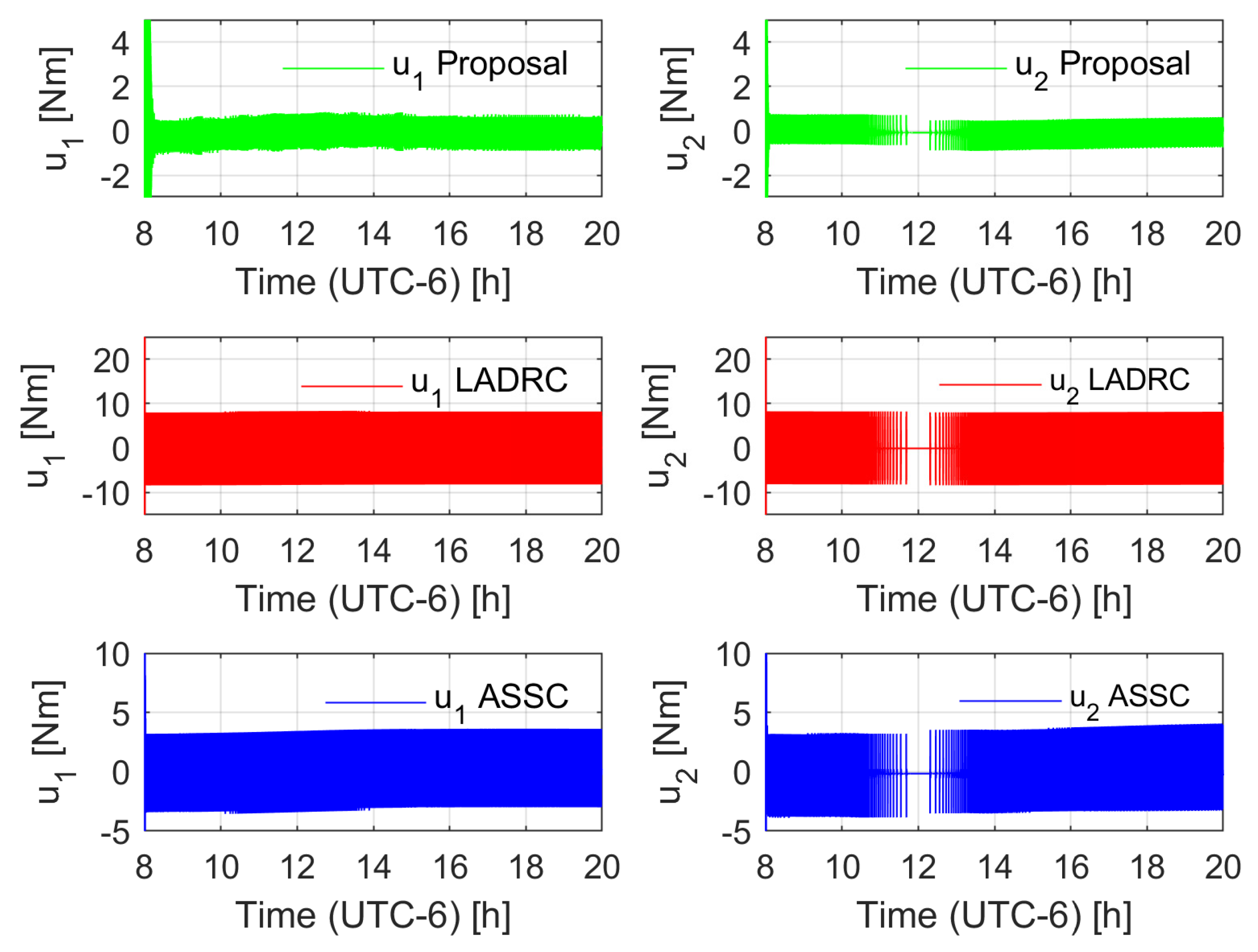
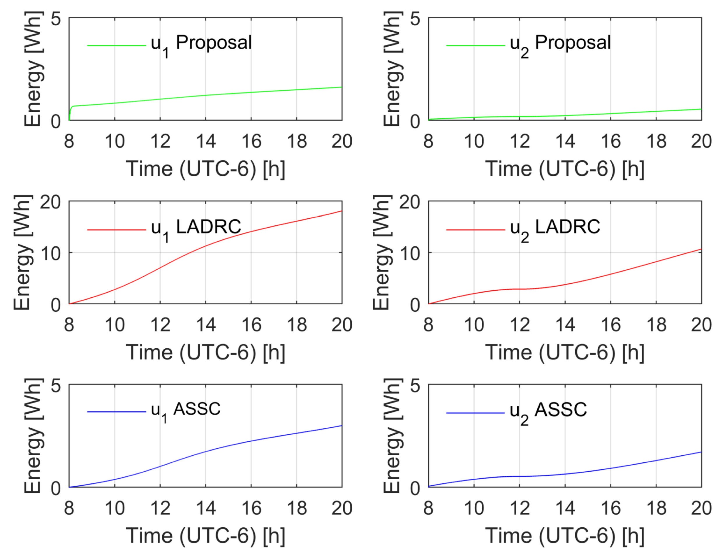
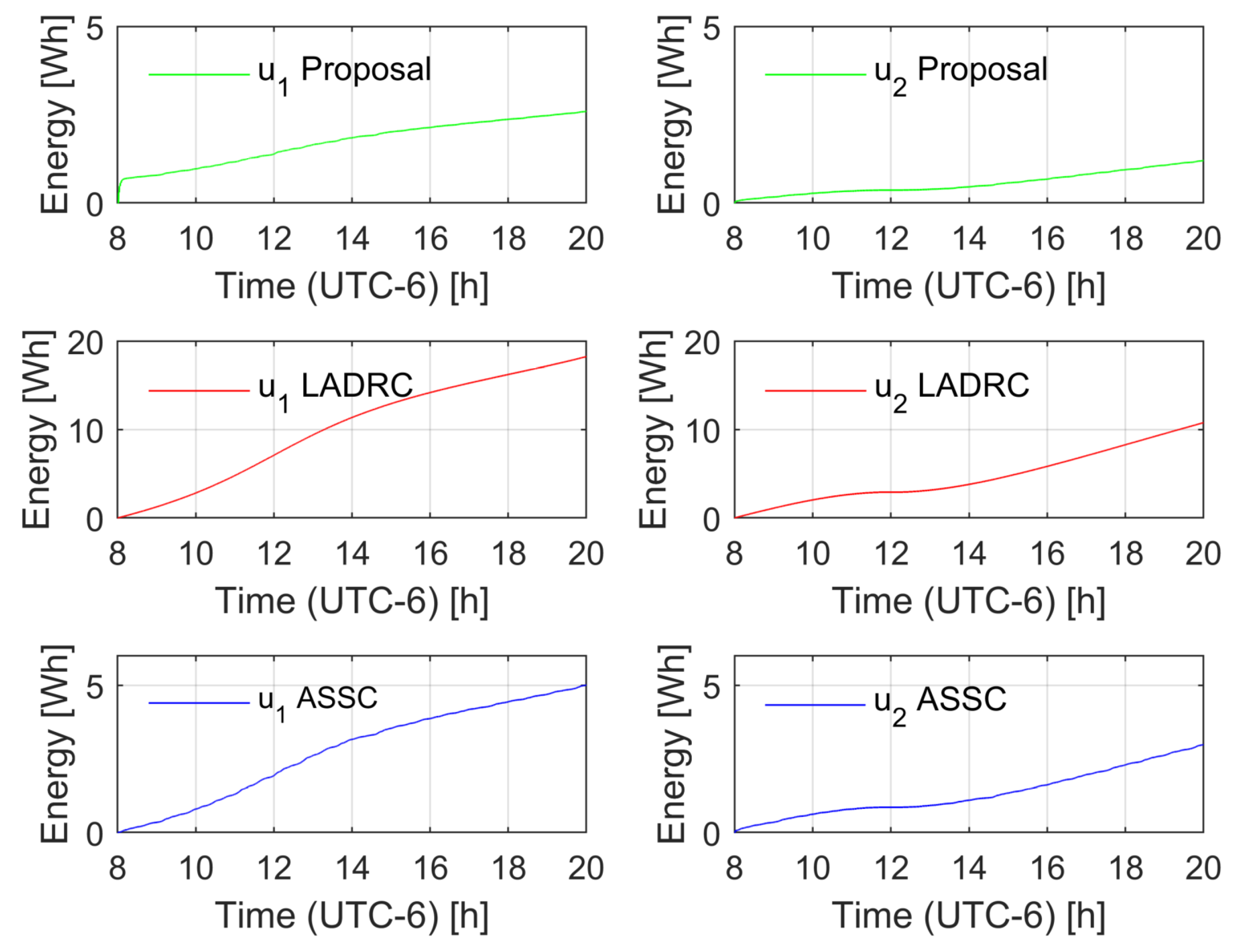
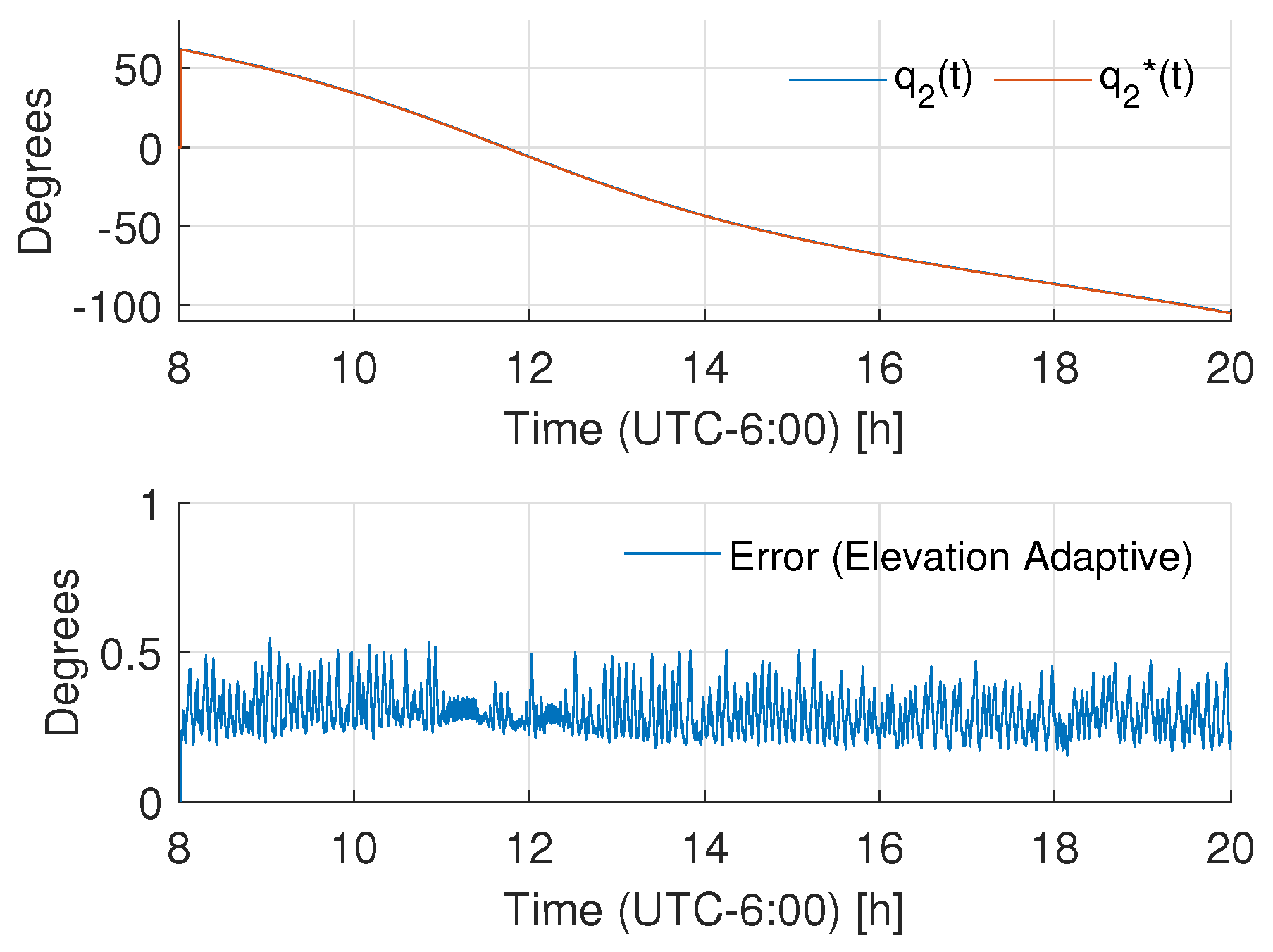
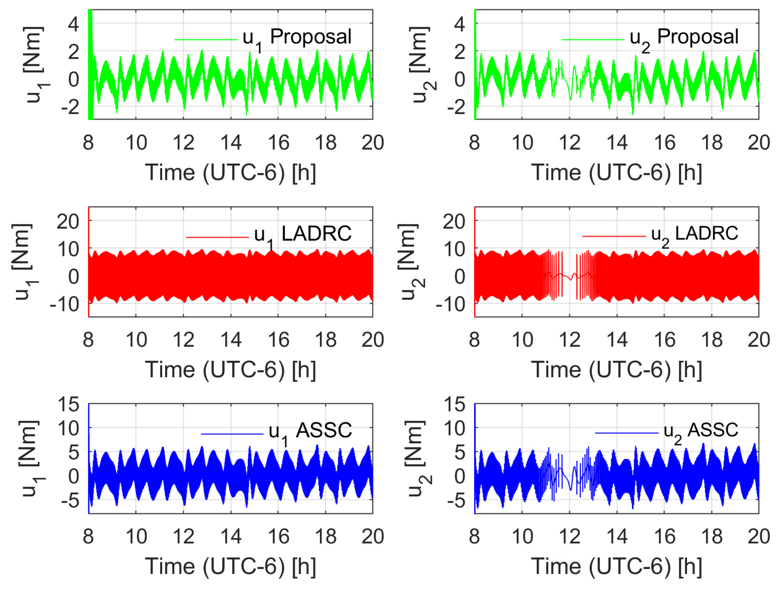
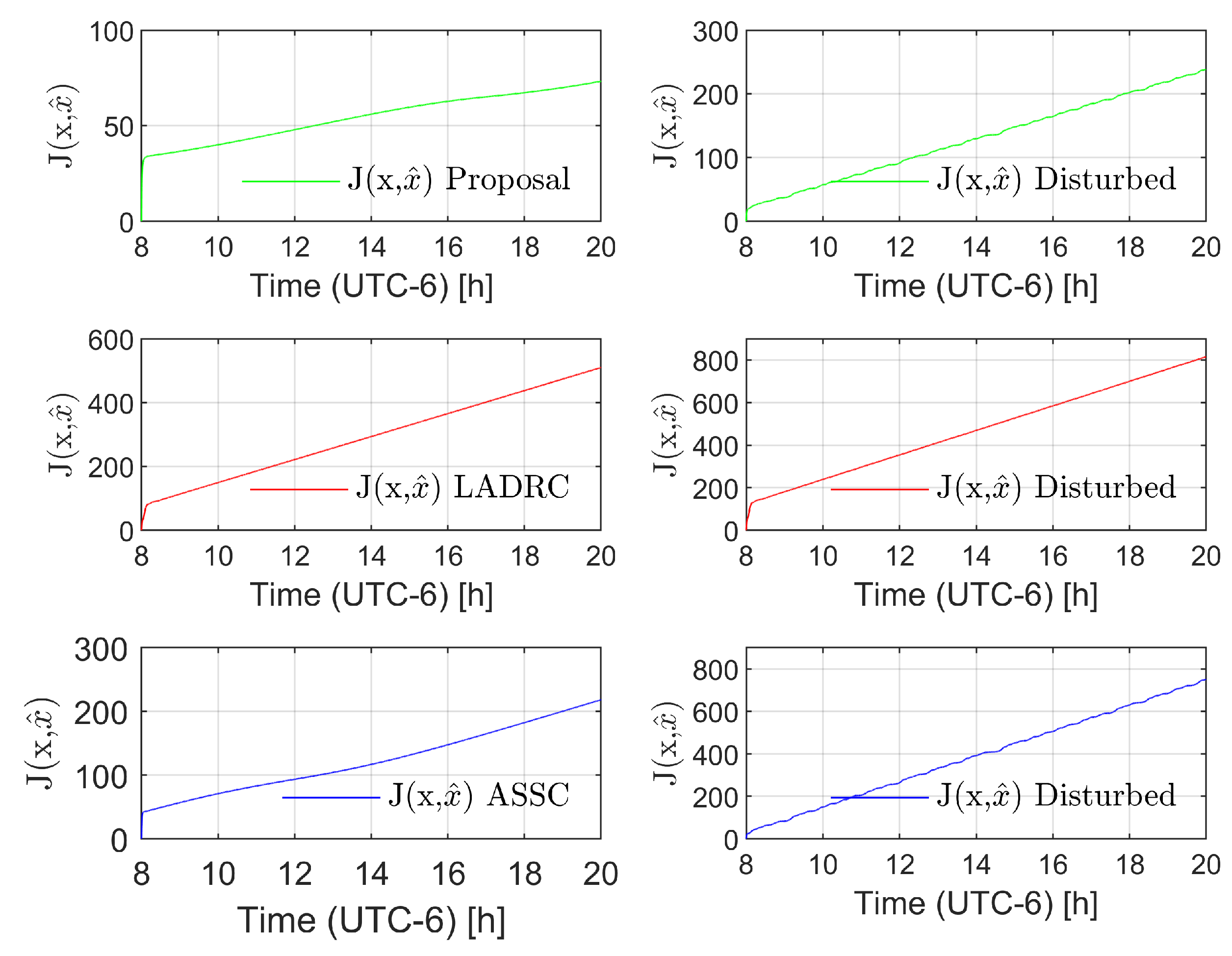
Some numerical and experimental tests show that the proposed controller demands a low energy consumption, in contrast to a classic ADRC scheme, while keeping appropriate estimation and tracking results for the solar tracking application.

The remainder of the article is given as follows. Section 2 presents the class of systems and the control problem. Section 3 provides the adaptive observer design and the stability test. Then, Section 4 presents the experimental results in the tracking of a numerically generated solar trajectory. Finally, Section 5 provides some concluding remarks and a general discussion of the contribution.

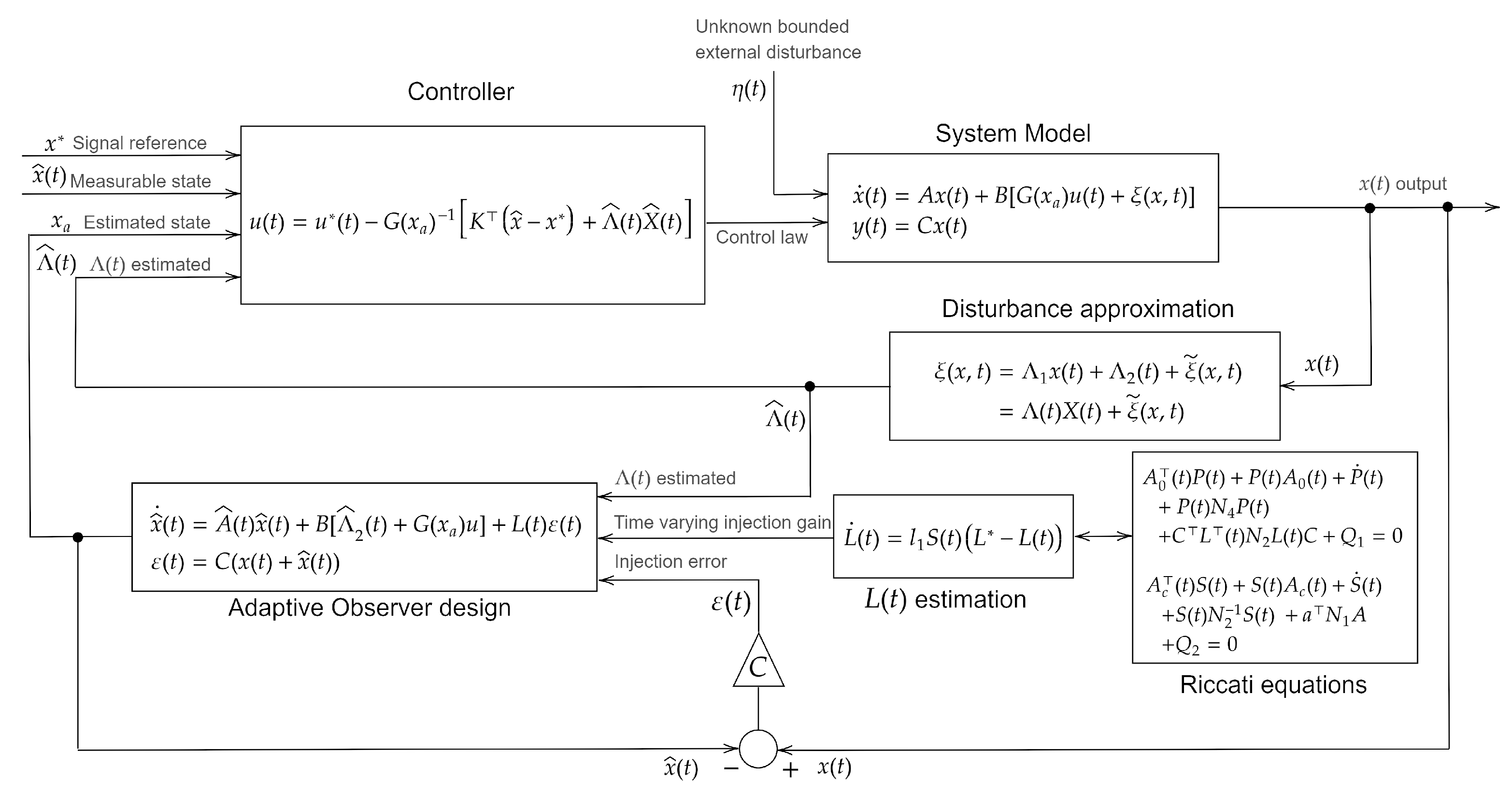
2. Controller Design

Consider the model which describes a class of open kinematic chain robotic manipulators:

$$\begin{array}{c}\hfill D\left(q\right)\ddot{q}+C(q,\dot{q})\dot{q}+g\left(q\right)=u+\eta \left(t\right)\end{array}$$

(1)

where $D\left(q\right)\in {\mathbb{R}}^{n\times n}$ is the inertia matrix (positive definite), $C(q,\dot{q})\in {\mathbb{R}}^{n\times n}$ is the coriolis matrix, $g\left(q\right)\in {\mathbb{R}}^n$ is the gravity vector, $u\in {\mathbb{R}}^n$ denotes the control input vector, and $\eta \left(t\right)\in {\mathbb{R}}^n$ denotes a vector of bounded external disturbances of unknown nature.

The last model can be represented as follows:

$$\begin{array}{cc}\hfill {\dot{x}}_a& =x_b\hfill \\ \hfill {\dot{x}}_b& =f\left(x\right)+G\left(x_a\right)u+\eta \left(t\right)\hfill \end{array}$$

(2)

where $x_a\left(t\right):=q\left(t\right)$, $x_b\left(t\right):=\dot{q}\left(t\right)$, $x\in {\mathbb{R}}^{2n}$, $x={\left[\begin{array}{cc}{x}_a^{⊺}& x_b^{⊺}\end{array}\right]}^{⊺}$ is the state vector, $G\left(x_a\right):=D{\left(q\right)}^{-1}$, which is always well defined from the positive definiteness condition on $D\left(q\right)$.

A direct consequence of the inertia matrix bounds property is the following inequality:

$$\begin{array}{c}\hfill 0<g^{-}\le \parallel G(·)\parallel \le g^{+},g^{-},g^{+}\in {\mathbb{R}}^{+}\end{array}$$

(3)

Assuming a lack of knowledge of the terms f and $\eta$, both terms can be lumped into a generalized disturbance input $\xi (x,t):=f\left(x\right)+\eta \left(t\right)$. Then, system (2) can be rewritten as

$$\begin{array}{cc}\hfill \dot{x}\left(t\right)& =Ax\left(t\right)+B\left[G\left(x_a\right)u\left(t\right)+\xi (x,t)\right]\hfill \\ \hfill y\left(t\right)& =Cx\left(t\right)\hfill \end{array}$$

(4)

where $y\in {\mathbb{R}}^{n\times 1}$, $y=x_a$ denotes the measurable output. $A\in {\mathbb{R}}^{2n\times 2n}$, $B\in {\mathbb{R}}^{2n\times n}$, $C\in {\mathbb{R}}^{n\times 2n}$ with values given by

$$\begin{array}{c}\hfill A=\left[\begin{array}{cc}{0}_{n\times n}& I_{n\times n}\\ 0_{n\times n}& 0_{n\times n}\end{array}\right],B=\left[\begin{array}{c}{0}_{n\times n}\\ I_{n\times n}\end{array}\right],C:=\left[\begin{array}{cc}{I}_{n\times n}& 0_{n\times n}\end{array}\right]\end{array}$$

(5)

Disturbance approximation: In this article, the generalized disturbance input is proposed to be approximated by the time varying combination of the system states and an additionally constant term (to incorporate arising offset contributions):

$$\begin{array}{cc}\hfill \xi (x,t)& ={\Lambda }_1\left(t\right)x\left(t\right)+{\Lambda }_2\left(t\right)+\tilde{\xi }(x,t)\hfill \\ \hfill & =\Lambda \left(t\right)X\left(t\right)+\tilde{\xi }(x,t)\hfill \end{array}$$

(6)

where $\Lambda \left(t\right)\in {\mathbb{R}}^{n\times 2n+1}$ is the time varying approximation matrix, $\Lambda \left(t\right)=\left[\begin{array}{cc}{\Lambda }_1\left(t\right)& {\Lambda }_2\left(t\right)\end{array}\right]$, with ${\Lambda }_1\left(t\right)\in {\mathbb{R}}^{n\times 2n}$ denoting the approximation based on the state vector and ${\Lambda }_2\left(t\right)\in {\mathbb{R}}^{n\times 1}$ representing the offset adjustment. The vector $X\in {\mathbb{R}}^{2n+1\times 1}$ is defined as $X:={\left[\begin{array}{cc}{x}^{⊺}& 1\end{array}\right]}^{⊺}$, and $\tilde{\xi }\in {\mathbb{R}}^n$ denotes the approximation error.

In this article, the approximation error is proposed to be minimized through a time window least squares criterion (see [49] for the single input-single output unbiased case).

3. Observer Design

The adaptive observer for the system (4) is proposed as

$$\begin{array}{cc}\hfill \dot{\widehat{x}}& =\widehat{A}\left(t\right)\widehat{x}\left(t\right)+B\left[{\widehat{\Lambda }}_2\left(t\right)+G\left(x_a\right)u\right]+L\left(t\right)\epsilon \left(t\right)\hfill \\ \hfill \epsilon \left(t\right)& =C\left(x\left(t\right)-\widehat{x}\left(t\right)\right)\hfill \\ \hfill \widehat{A}\left(t\right)& =\left[\begin{array}{c}{0}_{n\times n}{I}_{n\times n}\\ {\widehat{\Lambda }}_1\left(t\right)\end{array}\right]\hfill \end{array}$$

(7)

where $G\left(x_a\right)$ is used instead of $G\left({\widehat{x}}_a\right)$ since $x_a$ is a measurable state. The term $\widehat{x}\in {\mathbb{R}}^{2n}$ denotes the estimate of x, the matrix $C\in {\mathbb{R}}^{n\times 2n}$ maps the state vector to the measurable states $x_a$, $\epsilon \left(t\right)\in {\mathbb{R}}^n$ denotes the injection error, and $L\left(t\right)\in {\mathbb{R}}^{2n\times n}$ is the time varying injection gain subject to an adaptation law of the form:

$$\begin{array}{cc}\hfill \dot{L}\left(t\right)& =l_{1}S\left(t\right)\left(L^{*}-L\left(t\right)\right)\hfill \end{array}$$

(8)

where $l_1\in {\mathbb{R}}^{+}$ is a positive constant, and $S\left(t\right)\in {\mathbb{R}}^{2n\times 2n}$, $P\left(t\right)\in {\mathbb{R}}^{2n\times 2n}$ positive definite time varying matrices which satisfy the following Riccati equations:

$$\begin{array}{cc}\hfill A_o^{⊺}\left(t\right)P\left(t\right)+P\left(t\right)A_o\left(t\right)+\dot{P}\left(t\right)+P\left(t\right)N_{4}P\left(t\right)+C^{⊺}{L}^{⊺}\left(t\right)N_{2}L\left(t\right)C+Q_1& =0\hfill \end{array}$$

(9)

$$\begin{array}{cc}\hfill A_c^{⊺}S\left(t\right)+S\left(t\right)A_c+\dot{S}\left(t\right)+S\left(t\right)N_2^{-1}S\left(t\right)+A^{⊺}{N}_{1}A+Q_2& =0\hfill \end{array}$$

(10)

where $A_c=A-B{K}^{⊺}$, $A_o:=A-L\left(t\right)C$, and $N_2\in {\mathbb{R}}^{2n\times 2n}$, $N_2=N_2^{⊺}>0$. The term $L^{*}$ is a user defined parameter such that the matrix $A-L^{*}C$ is Hurwitz.

Control Law

Let $x^{*}\in {\mathbb{R}}^{2n}$ be a smooth reference trajectory for the state vector x. From the nominal dynamics (4) without the presence of disturbances, the feedforward input $u^{*}$ can be defined such that the following relation is satisfied:

$$\begin{array}{cc}\hfill {\dot{x}}^{*}\left(t\right)& =A{x}^{*}\left(t\right)+BG\left(x_a\right)u^{*}\left(t\right)\hfill \end{array}$$

(11)

which leads to

$$\begin{array}{cc}\hfill u^{*}\left(t\right)& =G{\left(x_a\right)}^{-1}{\dot{x}}_b^{*}\hfill \end{array}$$

(12)

The output-based control is proposed as

$$\begin{array}{c}\hfill u\left(t\right)=u^{*}\left(t\right)-G{\left(x_a\right)}^{-1}[K^{⊺}\left(\widehat{x}-x^{*}\right)+\widehat{\Lambda }\left(t\right)\widehat{X}\left(t\right)]\end{array}$$

(13)

where $K\in {\mathbb{R}}^{n\times 2n}$ is the control gain matrix and the last term of the control law stands for the estimate of the generalized disturbance input $\xi (x,t)$; that is, $\widehat{\xi }(x,t)=\widehat{\Lambda }\left(t\right)\widehat{X}\left(t\right)$. Figure 1 shows a block diagram of the proposed control structure.

The following result states the convergence of the tracking and estimation errors, in an ultimate bound sense, of the output based adaptive control law:

Theorem 1.

Consider the class of partially known robotic systems (4), where the lumped disturbance input $\xi (x,t)$ satisfies the condition of being absolutely bounded given a reference trajectory $x^{*}\left(t\right)$ and an output feedback control (13) based on a linear time varying identification of the disturbance input, given by (16), and an adaptive observer (7), such that the control gain K forces the matrix $A-B{K}^{⊺}$ to be Hurwitz. If there exist positive definite matrices $P\left(t\right),S\left(t\right)N_1,N_2,N_4,Q_1,Q_2\in {\mathbb{R}}^{2n\times 2n}$, such that the time varying Riccati Equations (9) and (10) have positive definitive solutions, the state estimation and tracking errors $\Delta \left(t\right)$ and $\delta \left(t\right)$ are uniformly ultimate bounded.

Proof. 

The estimation error obeys the following dynamics:

$$\begin{array}{cc}\hfill \dot{\Delta }\left(t\right)& =\left(A-L\left(t\right)C\right)\Delta \left(t\right)+A\widehat{x}\left(t\right)+B\tilde{\xi }(x,t)\hfill \\ \hfill & =(A-L\left(t\right)C)\Delta \left(t\right)+A\delta \left(t\right)+A{x}^{*}\left(t\right)+B\tilde{\xi }(x,t)\hfill \end{array}$$

(14)

Let define the difference between the estimate state $\widehat{x}$ and the desired trajectory $x^{*}$ as $\delta \left(t\right)$. The dynamics of $\delta \left(t\right)$ are computed as

$$\begin{array}{cc}\hfill \dot{\delta }\left(t\right)& =\left(A-B{K}^{⊺}\right)\delta \left(t\right)+L\left(t\right)C\Delta \left(t\right)\hfill \end{array}$$

(15)

From the observer dynamics (7) and the disturbance approximation proposal (6), the time varying approximation matrix $\widehat{\Lambda }\left(t\right)$ is proposed as the solution of the following optimization problem:

$$\begin{array}{cc}\hfill {\widehat{\Lambda }}^{*}\left(t\right)& =\underset{\widehat{\Lambda }\in {\mathbb{R}}^{n\times (2n+1)}}{argmin}{\left[{\int }_{t-\nu }^t\omega \left(\tau \right)-\widehat{\Lambda }\left(\tau \right)X\left(\tau \right)d\tau \right]}^2\hfill \\ \hfill & \mathrm{where}\hfill \end{array}$$

(16)

$$\begin{array}{cc}\hfill \omega \left(t\right)& =B^{⊺}\left[\widehat{x}\left(t\right)-\widehat{x}(t-\nu )\right]-\left[{\int }_{t-\nu }^{t}G\left(x_a\right)u\left(\tau \right)+B^{⊺}L\left(\tau \right)\epsilon \left(\tau \right)d\tau \right]\hfill \end{array}$$

(17)

whose solution leads to the following dynamics [51]:

$$\begin{array}{c}\hfill {\widehat{\Lambda }}^{⊺}\left(t\right)={[{\int }_{t-\nu }^t\widehat{X}\left(\tau \right){\widehat{X}}^{⊺}\left(\tau \right)d\tau ]}^{-1}{[{\int }_{t-\nu }^t\omega \left(\tau \right){\widehat{X}}^{⊺}\left(\tau \right)d\tau ]}^{⊺}\end{array}$$

(18)

Now, let us propose the following quadratic Lyapunov candidate function:

$$\begin{array}{cc}\hfill V& (\Delta ,\delta ,L,\rho ,K^{⊺},t)={\Delta }^{⊺}P\left(t\right)\Delta +{\delta }^{⊺}S\left(t\right)\delta +\mathrm{tr}\left\{{\displaystyle \frac{1}{2}}{l}_1^{-1}{\tilde{L}}^{⊺}\left(t\right)\tilde{L}\left(t\right)\right\}+\mathrm{tr}\left\{{\displaystyle \frac{1}{2}}{\rho }^{⊺}\left(t\right)\rho \left(t\right)\right\}\hfill \end{array}$$

(19)

where

$$\begin{array}{cc}\hfill \rho \left(t\right)& ={\int }_0^t\left[{\int }_{\tau -\nu }^{\tau }\widehat{x}\left(\sigma \right)\omega \left(\sigma \right)-{\int }_{\tau -\nu }^{\tau }\widehat{x}\left(\sigma \right){\widehat{x}}^{⊺}\left(\sigma \right)d\sigma \widehat{\Lambda }\left(\tau \right)\right]d\tau \hfill \end{array}$$

(20)

$$\begin{array}{cc}\hfill \tilde{L}\left(t\right)& =L^{*}-L\left(t\right)\hfill \end{array}$$

(21)

The time derivative of the Lyapunov candidate function (19) is given by

$$\begin{array}{cc}\hfill \dot{V}& (\Delta ,\delta ,L,\rho ,K^{⊺},t)={\Delta }^{⊺}\left[A_o^{⊺}\left(t\right)P\left(t\right)+P\left(t\right)A_o\left(t\right)+\dot{P}\left(t\right)\right]\Delta +\mathrm{tr}\left\{{\tilde{L}}^{⊺}\left(t\right)\dot{\tilde{L}}\left(t\right)\right\}+\hfill \\ \hfill & +{\delta }^{⊺}\left[A_c^{⊺}S\left(t\right)+S\left(t\right)A_c+\dot{S}\left(t\right)\right]\delta +{\delta }^{⊺}{A}^{⊺}P\left(t\right)\Delta +{\Delta }^{⊺}P\left(t\right)A\delta +{\Delta }^{⊺}{C}^{⊺}{L}^{⊺}\left(t\right)S\left(t\right)\delta \hfill \\ \hfill & +{\delta }^{⊺}{S}^{⊺}\left(t\right)L\left(t\right)C\Delta +{(A{x}^{*}+B\tilde{\epsilon })}^{⊺}P\left(t\right)\Delta +{\Delta }^{⊺}P\left(t\right)(A{x}^{*}+B\tilde{\epsilon })+\mathrm{tr}\left\{{\rho }^{⊺}\left(t\right)\dot{\rho }\left(t\right)\right\}\hfill \end{array}$$

(22)

From the lambda inequality [52], there exists a set of symmetric positive definite matrices $N_i\in {\mathbb{R}}^{2n\times 2n},i=1,2,3,$ such that

$$\begin{array}{cc}\hfill {\delta }^{⊺}{A}^{⊺}P\left(t\right)\Delta +{\Delta }^{⊺}P\left(t\right)A\delta \le & {\delta }^{⊺}{A}^{⊺}{N}_{1}A\delta +\hfill \\ \hfill & +{\Delta }^{⊺}P\left(t\right)N_1^{-1}P\left(t\right)\Delta \hfill \end{array}$$

(23)

$$\begin{array}{cc}\hfill {\Delta }^{⊺}{C}^{⊺}{L}^{⊺}\left(t\right)S\left(t\right)\delta +{\delta }^{⊺}S\left(t\right)L\left(t\right)C\Delta \le & {\Delta }^{⊺}{C}^{⊺}{L}^{⊺}\left(t\right)N_{2}L\left(t\right)C\Delta +\hfill \\ \hfill & +{\delta }^{⊺}S\left(t\right)N_2^{-1}S\left(t\right)\delta \hfill \end{array}$$

(24)

$$\begin{array}{cc}\hfill {(A{x}^{*}+B\tilde{\epsilon })}^{⊺}P\left(t\right)\Delta +{\Delta }^{⊺}P\left(t\right)(A{x}^{*}+B\tilde{\epsilon })\le & {(A{x}^{*}+B\tilde{\epsilon })}^{⊺}{N}_3(A{x}^{*}+B\tilde{\epsilon })+\hfill \\ \hfill & +{\Delta }^{⊺}P\left(t\right)N_3^{-1}P\left(t\right)\Delta \hfill \end{array}$$

(25)

Using (23)–(25) in (22),

$$\begin{array}{cc}\hfill \dot{V}(\Delta ,\delta ,L,\rho ,K^{⊺},t)& ={\Delta }^{⊺}[A_o^{⊺}\left(t\right)P\left(t\right)+P\left(t\right)A_o\left(t\right)+\dot{P}\left(t\right)+P\left(t\right)N_1^{-1}P\left(t\right)+\hfill \\ \hfill & +C^{⊺}{L}^{⊺}\left(t\right)N_{2}L\left(t\right)C+P\left(t\right)N_3^{-1}P\left(t\right)]\Delta +\hfill \\ \hfill & +{\delta }^{⊺}\left[A_c^{⊺}S\left(t\right)+S\left(t\right)A_c+\dot{S}\left(t\right)+A^{⊺}{N}_{1}A+S\left(t\right)N_2^{-1}S\left(t\right)\right]\delta +\hfill \\ \hfill & +{(A{x}^{*}+B\tilde{\epsilon })}^{⊺}{N}_3(A{x}^{*}+B\tilde{\epsilon })+\mathrm{tr}\left\{{\rho }^{⊺}\left(t\right)\dot{\rho }\left(t\right)\right\}+\mathrm{tr}\left\{{\tilde{L}}^{⊺}\left(t\right)\dot{\tilde{L}}\left(t\right)\right\}\hfill \end{array}$$

(26)

Since $N_1,N_2$ are positive definite, the terms $A^{⊺}{N}_{1}A$, $C^{⊺}{L}^{⊺}\left(t\right)N_{2}L\left(t\right)C$ are positive definite (see Section 7.1 of [53]). Then, to complete the time varying Riccati equations while ensuring the negative definiteness condition of the time derivative of V, let us add $\pm {\Delta }^{⊺}\left(t\right)Q_1\Delta \pm {\delta }^{⊺}{Q}_2\delta$, for symmetric positive definite matrices $Q_1,Q_2\in {\mathbb{R}}^{2n\times 2n}$. Then, we obtain

$$\begin{array}{cc}\hfill \dot{V}(\Delta ,& \delta ,L,\rho ,K^{⊺},t)={\Delta }^{⊺}[A_o^{⊺}\left(t\right)P\left(t\right)+P\left(t\right)A_o\left(t\right)+\dot{P}\left(t\right)+P\left(t\right)N_{4}P\left(t\right)+\hfill \\ \hfill & \hfill +C^{⊺}{L}^{⊺}\left(t\right)N_{2}L\left(t\right)C+Q_1]\Delta +{\delta }^{⊺}[A_c^{⊺}S\left(t\right)+S\left(t\right)A_c+\dot{S}\left(t\right)+S\left(t\right)N_2^{-1}S\left(t\right)+\\ \hfill & +A^{⊺}{N}_{1}A+Q_2]\delta +{(A{x}^{*}+B\tilde{\epsilon })}^{⊺}{N}_3(A{x}^{*}+B\tilde{\epsilon })+\mathrm{tr}\left\{{\rho }^{⊺}\left(t\right)\dot{\rho }\left(t\right)\right\}+\hfill \\ \hfill & +\mathrm{tr}\left\{{\tilde{L}}^{⊺}\left(t\right)\dot{\tilde{L}}\left(t\right)\right\}-{\Delta }^{⊺}{Q}_1\Delta -{\delta }^{⊺}{Q}_2\delta \hfill \end{array}$$

(27)

where $N_4=N_1^{-1}+N_3^{-1}$. Using the dynamics (18), the following equality is obtained:

$$\begin{array}{c}\hfill {\int }_{t-\nu }^t\widehat{x}\left(\tau \right)\omega \left(\tau \right)d\tau -{\int }_{t-\nu }^t\widehat{x}\left(\tau \right){\widehat{x}}^{⊺}\left(\tau \right)d\tau \widehat{\Lambda }\left(t\right)=0\end{array}$$

(28)

which implies that ${\eta }^{⊺}\left(t\right)\dot{\eta }\left(t\right)=0$ (see [49]). From (8),

$$\begin{array}{c}\hfill \mathrm{tr}\left\{{\tilde{L}}^{⊺}\left(t\right)\dot{\tilde{L}}\left(t\right)\right\}=-\mathrm{tr}\left\{{\tilde{L}}^{⊺}\left(t\right)S\left(t\right)\tilde{L}\left(t\right)\right\}\end{array}$$

(29)

Since ${\tilde{L}}^{⊺}\left(t\right)S\left(t\right)\tilde{L}\left(t\right)$ is at least positive semidefinite (positive definite if $\tilde{L}\left(t\right)$ is full rank in columns), then (29) is negative or zero. Using (28) and (29) in (26), the following expression is obtained:

$$\begin{array}{cc}\hfill \dot{V}(\Delta ,\delta ,& L,\rho ,K^{⊺},t)={\Delta }^{⊺}[A_o^{⊺}\left(t\right)P\left(t\right)+P\left(t\right)A_o\left(t\right)+\dot{P}\left(t\right)+P\left(t\right)N_{4}P\left(t\right)+\hfill \\ \hfill & +C^{⊺}{L}^{⊺}\left(t\right)N_{2}L\left(t\right)C+Q_1]\Delta +{\delta }^{⊺}[A_c^{⊺}S\left(t\right)+S\left(t\right)A_c+\dot{S}\left(t\right)+\hfill \\ \hfill & +S\left(t\right)N_2^{-1}S\left(t\right)+A^{⊺}{N}_{1}A+Q_2]\delta +{(A{x}^{*}+B\tilde{\epsilon })}^{⊺}{N}_3(A{x}^{*}+B\tilde{\epsilon })-\hfill \\ \hfill & -\mathrm{tr}\left\{{\tilde{L}}^{⊺}\left(t\right)S\left(t\right)\tilde{L}\left(t\right)\right\}-{\Delta }^{⊺}{Q}_1\Delta -{\delta }^{⊺}{Q}_2\delta \hfill \end{array}$$

(30)

Using the assumption of the positive definiteness of the solutions of the Equations (9) and (10),

$$\begin{array}{cc}\hfill \dot{V}& (\Delta ,\delta ,L,\rho ,K^{⊺},t)={(A{x}^{*}+B\tilde{\epsilon })}^{⊺}{N}_3(A{x}^{*}+B\tilde{\epsilon })-\mathrm{tr}\left\{{\tilde{L}}^{⊺}\left(t\right)S\left(t\right)\tilde{L}\left(t\right)\right\}-{\Delta }^{⊺}{Q}_1\Delta -{\delta }^{⊺}{Q}_2\delta \hfill \end{array}$$

(31)

Let define the vectors z and $\tilde{z}$ as

$$\begin{array}{cc}\hfill z& :=\left[\begin{array}{c}\Delta \\ \delta \end{array}\right]\hfill \end{array}$$

(32)

$$\begin{array}{cc}\hfill \tilde{z}& :=A{x}^{*}+B\tilde{\epsilon }\hfill \end{array}$$

(33)

From the last definitions, (31) becomes

$$\begin{array}{cc}\hfill \dot{V}& (z,L,K^{⊺},t)={\tilde{z}}^{⊺}{N}_3\tilde{z}-\mathrm{tr}\left\{{\tilde{L}}^{⊺}\left(t\right)S\left(t\right)\tilde{L}\left(t\right)\right\}-z^{⊺}{Q}_{3}z\hfill \end{array}$$

(34)

with

$$\begin{array}{c}\hfill Q_3:=\left[\begin{array}{cc}{Q}_1& 0\\ 0& Q_2\end{array}\right]\end{array}$$

(35)

Using the Rayleigh inequality

$$\begin{array}{cc}\hfill \dot{V}(z,L,K^{⊺}& ,t)\le -{\lambda }_{min}\left(Q_3\right){\parallel z\parallel }^2-\mathrm{tr}\left\{{\tilde{L}}^{⊺}\left(t\right)S\left(t\right)\tilde{L}\left(t\right)\right\}+{\lambda }_{max}\left(N_3\right){\parallel \tilde{z}\parallel }^2\hfill \end{array}$$

(36)

Let us introduce the auxiliary term $\theta \in (0,1)$. Rewriting (36),

$$\begin{array}{cc}\hfill \dot{V}(z,L,K^{⊺},t)\le & -(1-\theta ){\lambda }_{min}\left(Q_3\right){\parallel z\parallel }^2-\theta {\lambda }_{min}\left(Q_3\right){\parallel z\parallel }^2-\hfill \\ \hfill & -\mathrm{tr}\left\{{\tilde{L}}^{⊺}\left(t\right)S\left(t\right)\tilde{L}\left(t\right)\right\}+{\lambda }_{max}\left(N_3\right){\parallel \tilde{z}\parallel }^2\hfill \end{array}$$

(37)

Then,

$$\begin{array}{cc}\hfill \dot{V}(z,L,K^{⊺},t)& \le -(1-\theta ){\lambda }_{min}\left(Q_3\right){\parallel z\parallel }^2-\mathrm{tr}\left\{{\tilde{L}}^{⊺}\left(t\right)S\left(t\right)\tilde{L}\left(t\right)\right\}<0;\hfill \\ \hfill & {\mathrm{for}\mathrm{all}\parallel z\parallel }^2\ge {\displaystyle \frac{{\lambda }_{max}\left(N_3\right){\parallel \tilde{z}\parallel }^2}{\theta {\lambda }_{min}\left(Q_3\right)}}\hfill \end{array}$$

From the last expression and using Definition 4.6 from [54], it is proven that the tracking and estimation errors are uniformly ultimately bounded. □

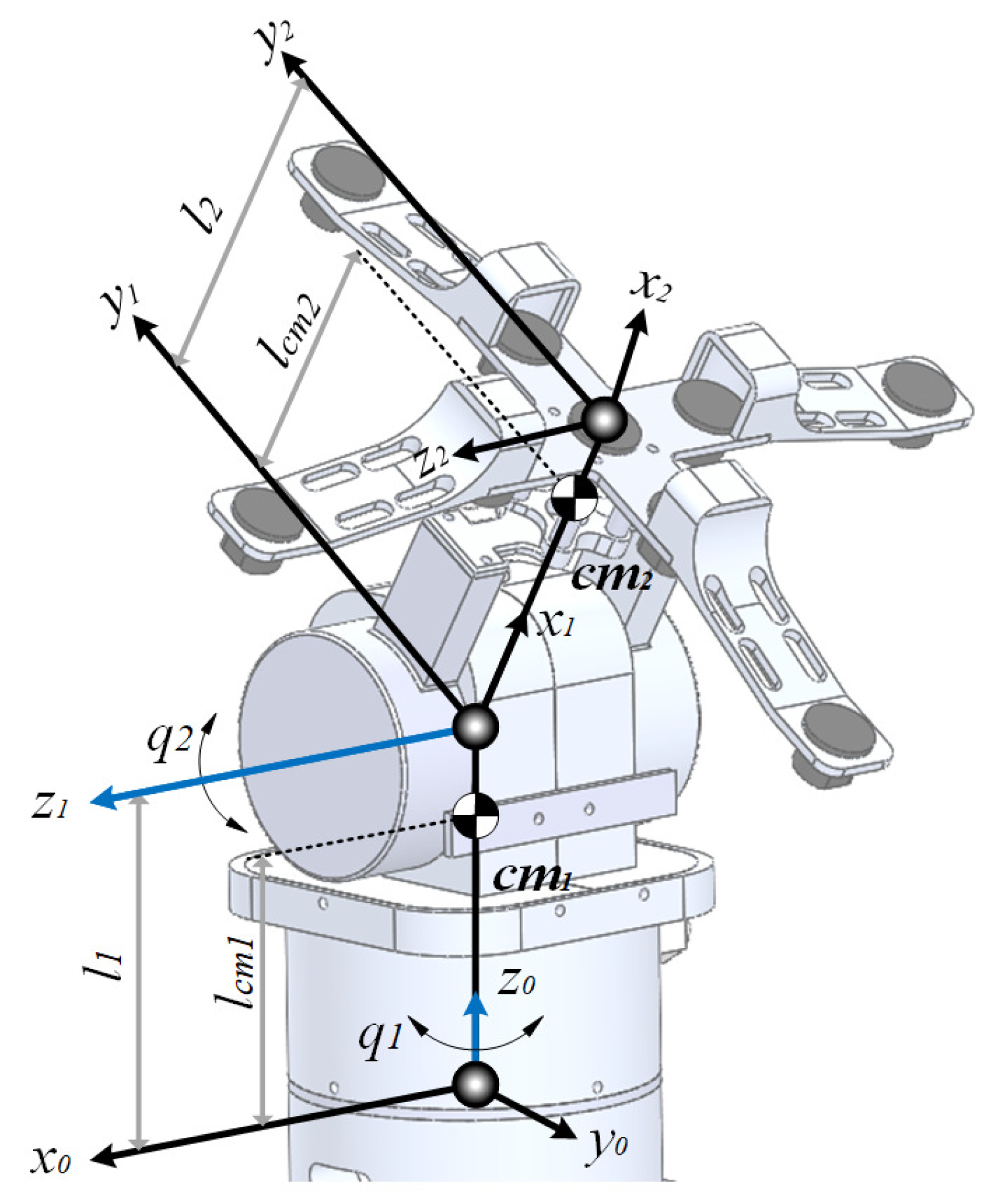
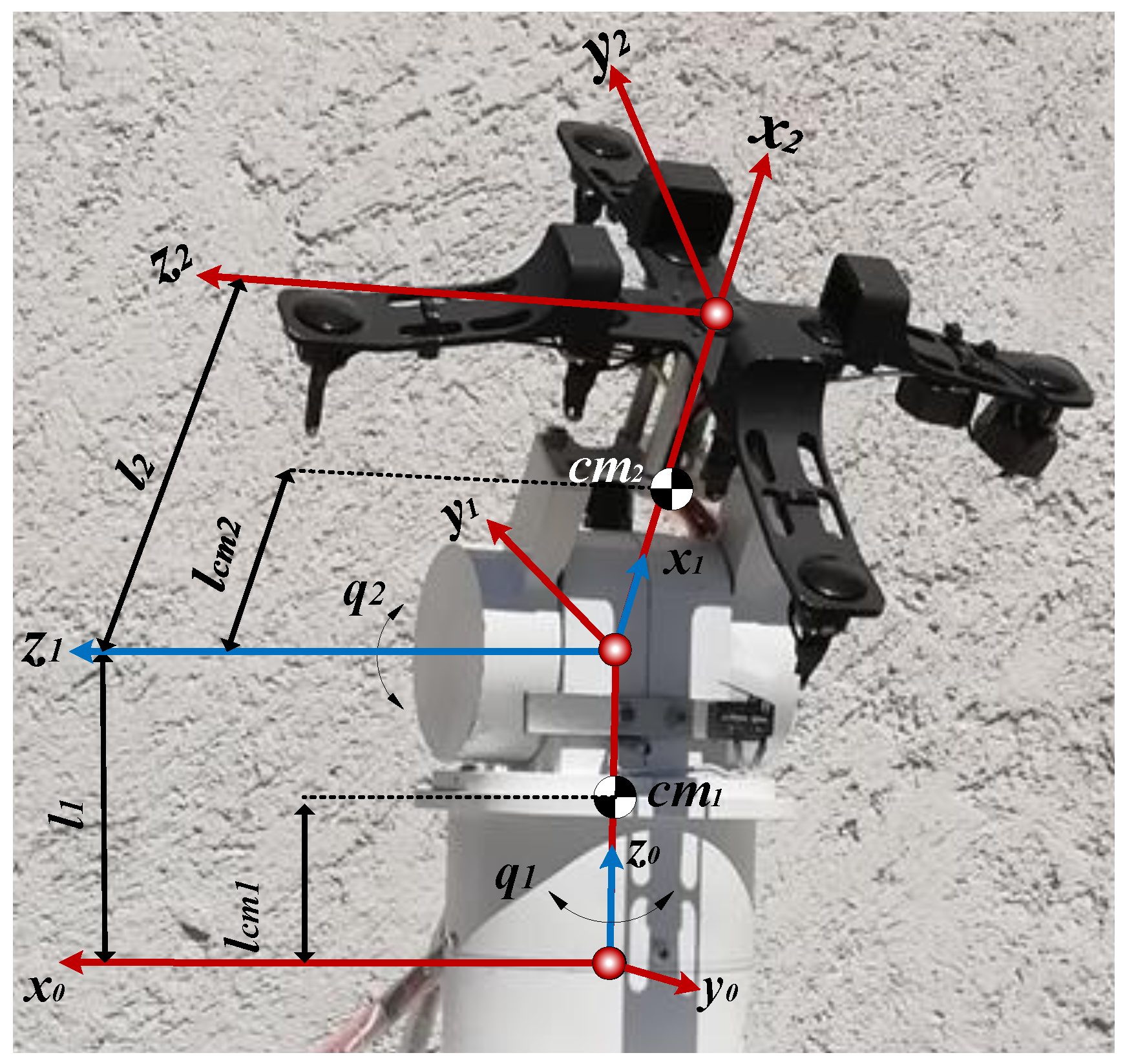
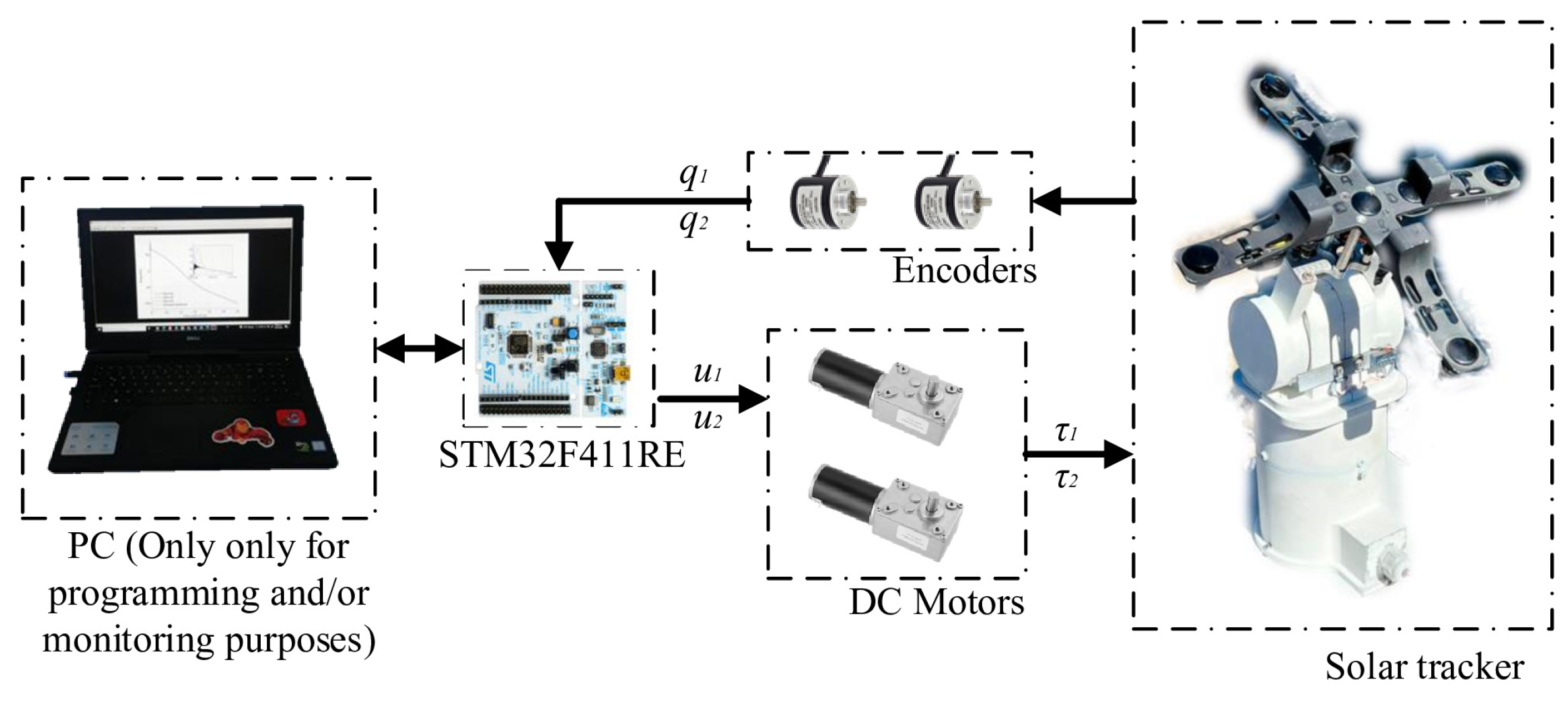
4. Case Study: A Two Degrees of Freedom Solar Tracker

Consider a two degrees of freedom solar tracking system in an azimuthal elevation configuration, the axis representation of which is given in Figure 2. The frames $\left\{0\right\}$, $\left\{1\right\}$, and $\left\{2\right\}$ denote the inertia, the azimuth link, and the end effector frame, respectively. Variables $m_i$, $I_i=\mathrm{diag}\{I_{xi},I_{yi},I_{zi}\}$ stand for the mass and Inertia tensor of the $i-th$ link (it is assumed to be diagonal since the links are assumed to besymmetric with respect to their center of mass). $\overline{g}$ denotes the gravity vector, $l_{cmi}$ is the distance from the previous frame ($i-1$) to the center of mass of the $i-th$ link, and $l_i$ is the length of the $i-th$ link, respectively.

Using the Euler Lagrange procedure, the dynamic model of the system in the form (1) is given as follows [55]:

$$\begin{array}{cc}\hfill & \left[\begin{array}{cc}{d}_{11}\left(q_2\right)& 0\\ 0& d_{22}\end{array}\right]\left[\begin{array}{c}{\ddot{q}}_1\\ {\ddot{q}}_2\end{array}\right]+\left[\begin{array}{cc}{c}_{11}(q_2,{\dot{q}}_2)& c_{12}(q_2,{\dot{q}}_1)\\ c_{21}(q_2,{\dot{q}}_1)& 0\end{array}\right]\left[\begin{array}{c}{\dot{q}}_1\\ {\dot{q}}_2\end{array}\right]+\left[\begin{array}{c}0\\ g_2\left(q_2\right)\end{array}\right]=\left[\begin{array}{c}{u}_1\\ u_2\end{array}\right]\hfill \\ \hfill & d_{11}\left(q_2\right):=(m_2{l}_{cm2}^2+I_{y2}){cos}^2\left(q_2\right)+I_{x2}{sin}^2\left(q_2\right)+I_{y1}\hfill \\ \hfill & d_{22}:=m_2{l}_{cm2}^2+I_{z2}\hfill \\ \hfill & c_{11}(q_2,{\dot{q}}_2):=cos\left(q_2\right)sin\left(q_2\right)(m_2{l}_{cm2}^2+I_{y2}-I_{x2}){\dot{q}}_2\hfill \\ \hfill & c_{12}(q_2,{\dot{q}}_1):=(I_{x2}-I_{y2}-m_2{l}_{cm2}^2)cos\left(q_2\right)sin\left(q_2\right){\dot{q}}_1\hfill \\ \hfill & c_{21}(q_2,{\dot{q}}_1):=-c_{12}(q_2,{\dot{q}}_1)\hfill \\ \hfill & g_2\left(q_2\right):=m_2{g}_r{l}_{cm2}cos\left(q_2\right)\hfill \end{array}$$

(38)

where $g_r$ stands for the gravity constant.

Let define the variables $x_a={\left[\begin{array}{cc}{x}_{a1}& x_{a2}\end{array}\right]}^{⊺}:={\left[\begin{array}{cc}{q}_1& q_2\end{array}\right]}^{⊺}$, $x_b={\left[\begin{array}{cc}{x}_{b1}& x_{b2}\end{array}\right]}^{⊺}:={\left[\begin{array}{cc}{\dot{q}}_1& {\dot{q}}_2\end{array}\right]}^{⊺}$. Then, the system (38) can be expressed as the class of systems (2) as follows:

$$\begin{array}{cc}\hfill {\dot{x}}_a& =x_b\hfill \end{array}$$

(39)

$$\begin{array}{cc}\hfill {\dot{x}}_b& =f\left(x\right)+G\left(x_a\right)u\hfill \end{array}$$

(40)

where

$$\begin{array}{cc}\hfill f\left(x\right)& =\left[\begin{array}{c}-{\displaystyle \frac{1}{d_{11}\left(x_{a2}\right)}}\left[c_{11}\left(x_{a2},x_{b2}\right)x_{b1}+c_{12}(x_{a2},x_{b1})x_{b2}\right]\\ -{\displaystyle \frac{1}{d_{22}}}\left[c_{21}\left(x_{a2},x_{b1}\right)x_{b1}+g_2\left(x_{a2}\right)\right]\end{array}\right],\hfill \\ \hfill G\left(x_a\right)& =\left[\begin{array}{cc}{\displaystyle \frac{1}{d_{11}\left(x_{a2}\right)}}& 0\\ 0& {\displaystyle \frac{1}{d_{22}}}\end{array}\right]\hfill \end{array}$$

4.1. System and Control Parameters

Since system (38) satisfies the class of systems to be controlled by the adaptive scheme (13), for this application, the following conditions were proposed:

• The parameters of the robotic system are provided in

  Table 1. Physical parameters of the robotic system.

  Parameter	Value
  $l_1$	100 mm
  $l_2$	120 mm
  $l_{cm1}$	61 mm
  $l_{cm2}$	104 mm
  $m_1$	$0.908$ Kg
  $m_2$	$0.290$ Kg
  $I_{y1}$	$0.01$ g·mm${}^2$
  $I_{x2}$	$0.04$ g·mm${}^2$
  $I_{y2}$	$0.01$ g·mm${}^2$
  $I_{z2}$	$0.95$ g·mm${}^2$
  $g_r$	$9.81$ Kg·m/s${}^2$

  .
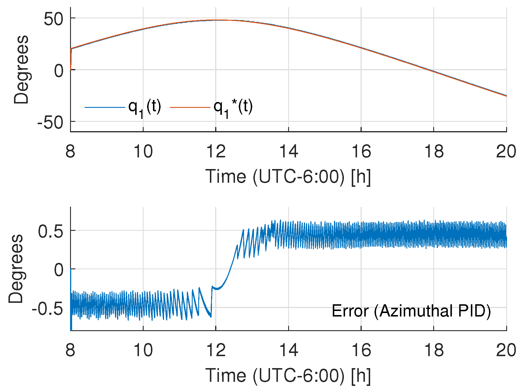
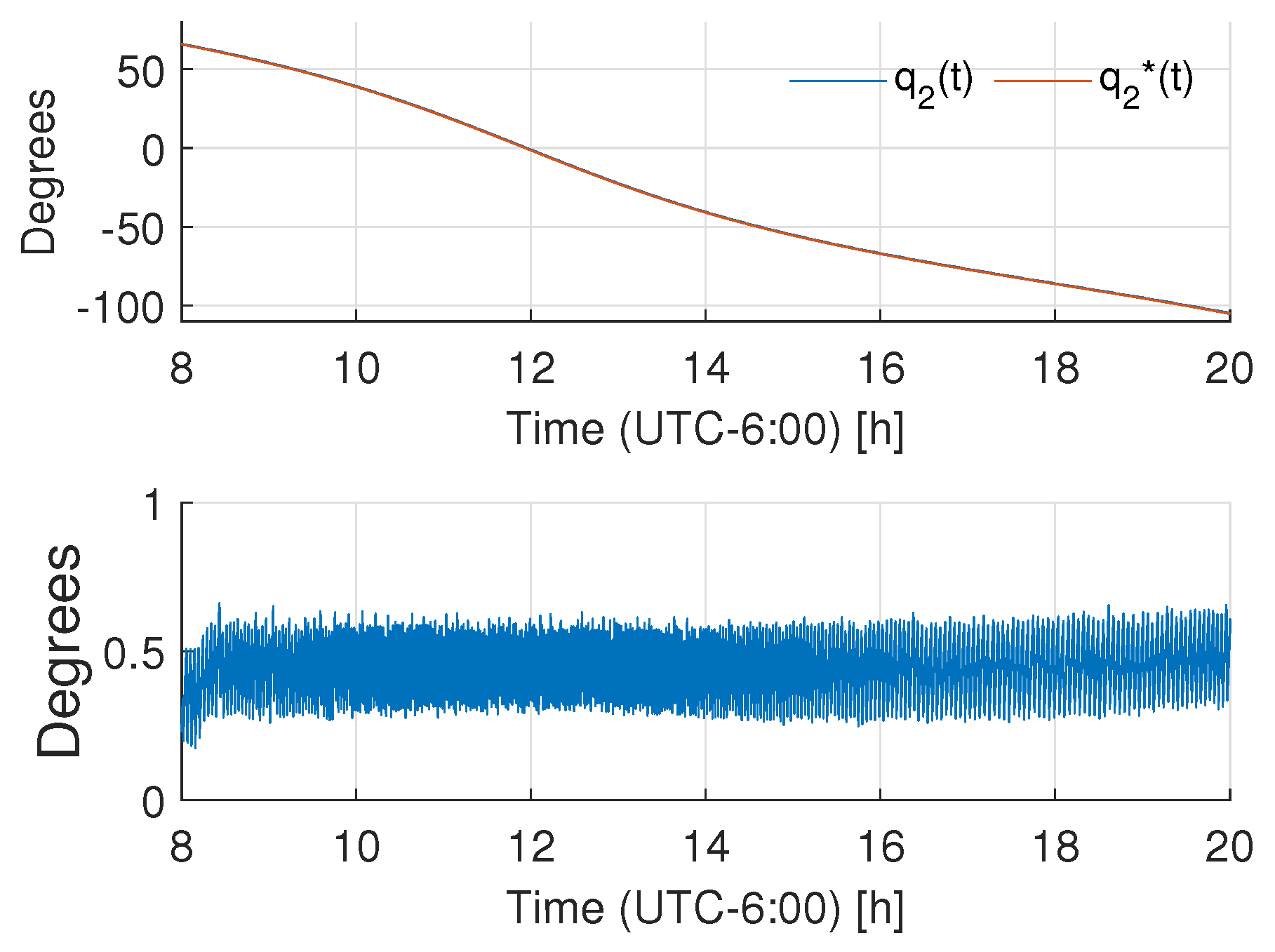
• The reference trajectory is defined by the Cooper’s algorithm [56], given by

  $$\begin{array}{cc}\hfill {\delta }_r& =23.45°sin\left(360\left({\displaystyle \frac{284+n}{365}}\right)\right)\hfill \\ \hfill q_2^{*}& =arcsin\left(cos({\varphi }_{r}cos\left({\delta }_r\right)cos\left({\sigma }_r\right))+sin\left({\varphi }_r\right)sin\left({\delta }_r\right)\right)\hfill \\ \hfill q_1^{*}& =arccos\left({\displaystyle \frac{sin\left(q_1^{*}\right)sin\left({\varphi }_r\right)-sin\left({\delta }_r\right)}{cos\left(q_2^{*}\right)cos\left({\varphi }_r\right)}}\right)\hfill \end{array}$$

  where ${\sigma }_r=(12-t)\left({15}^{\circ }\right)$, ${\delta }_r$ is the solar declination, ${\varphi }_r,L_{rc}$ are the longitude and latitude coordinates of the robot, n is the day number ($1<n<365$), and ${\sigma }_r$ denotes the hour angle. In this case, $n=93$, ${\varphi }_r=-99.12°$, $L_{rc}=19.12°$. The time interval, t, was set to be from 8 a.m. to 8 p.m.
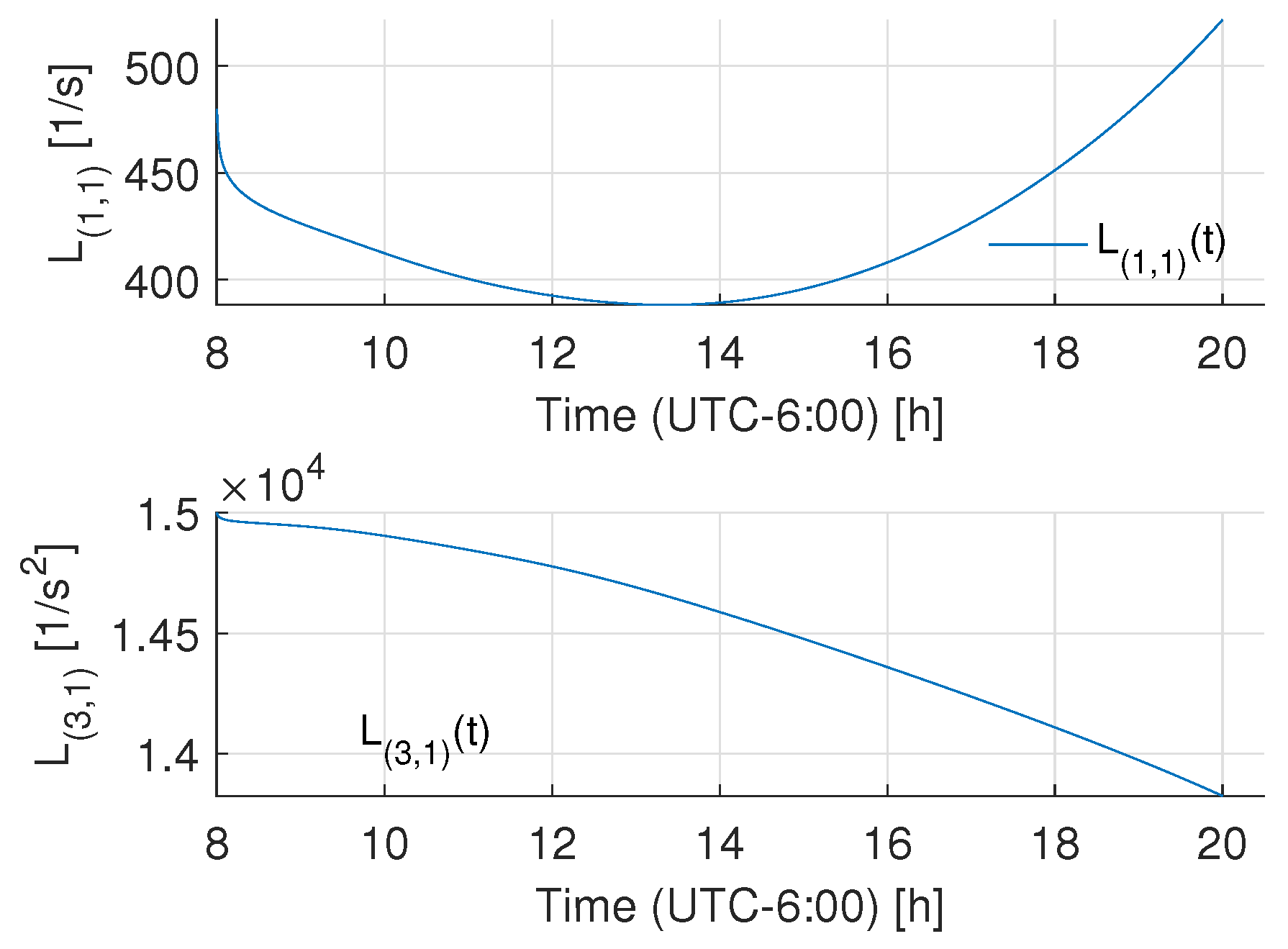
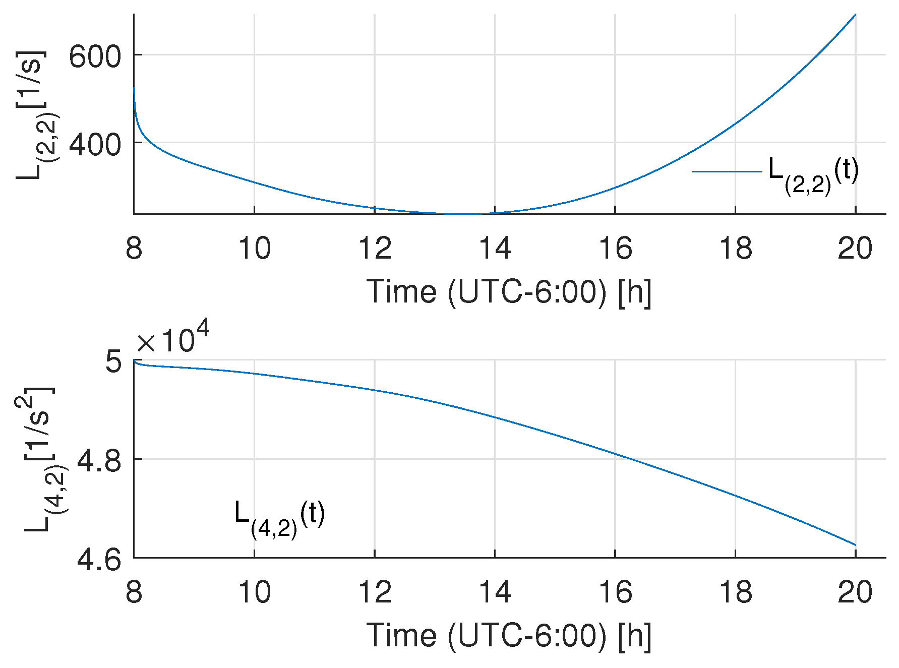
• The controller gain parameters were set to be

  $$\begin{array}{c}\hfill l_1=0.1;K^{⊺}=\left[\begin{array}{cccc}69& 0& 0.9& 0\\ 0& 69& 0& 0.9\end{array}\right];\\ \hfill {\left(L^{*}\right)}^{⊺}=\left[\begin{array}{cccc}400& 0& 1.4\times {10}^4& 0\\ 0& 400& 0& 4.5\times {10}^4\end{array}\right]\end{array}$$
  The choice of $L^{*}$, $l_1$, $K^{⊺}$ was in the context of a set of a model matching with two decoupled, stable, second-order linear model references of the form $s^2+2{\zeta }_i{\omega }_{ni}s+{\omega }_{ni}^2$, $i=1,2$, ${\zeta }_i,{\omega }_{ni}>0$. That is,

  $$\begin{array}{cc}\hfill K^{⊺}& =\left[\begin{array}{cccc}2{\zeta }_{1c}{\omega }_{n1c}& 0& {\omega }_{n1c}^2& 0\\ 0& 2{\zeta }_{2c}{\omega }_{n2c}& 0& {\omega }_{n2c}^2\end{array}\right]\hfill \\ \hfill {\left(L^{*}\right)}^{⊺}& =l_1\left[\begin{array}{cccc}2{\zeta }_{1o}{\omega }_{n1o}& 0& {\omega }_{n1o}^2& 0\\ 0& 2{\zeta }_{2o}{\omega }_{n2o}& 0& {\omega }_{n2o}^2\end{array}\right]\hfill \end{array}$$

  where ${\zeta }_{1c}={\zeta }_{2c}=36.3662$, ${\omega }_{n1c}={\omega }_{n2c}=0.9487$, ${\zeta }_{1c}={\zeta }_{2c}=0.5345$, ${\omega }_{n1c}={\omega }_{n2c}=37.4166$. This choice can be enhanced by optimization procedures [57], but this aspect is out of the scope of this work and will be considered in future research.

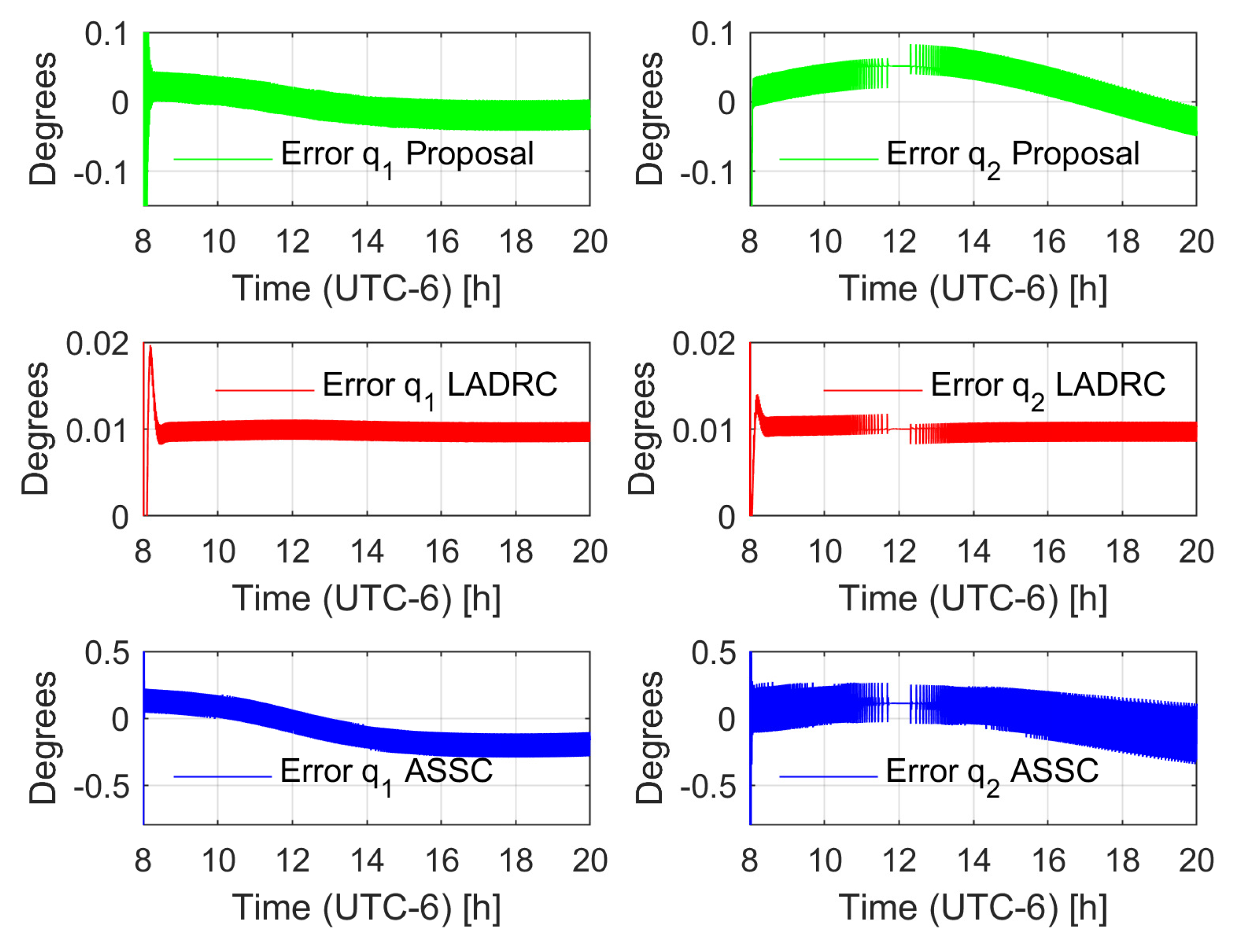
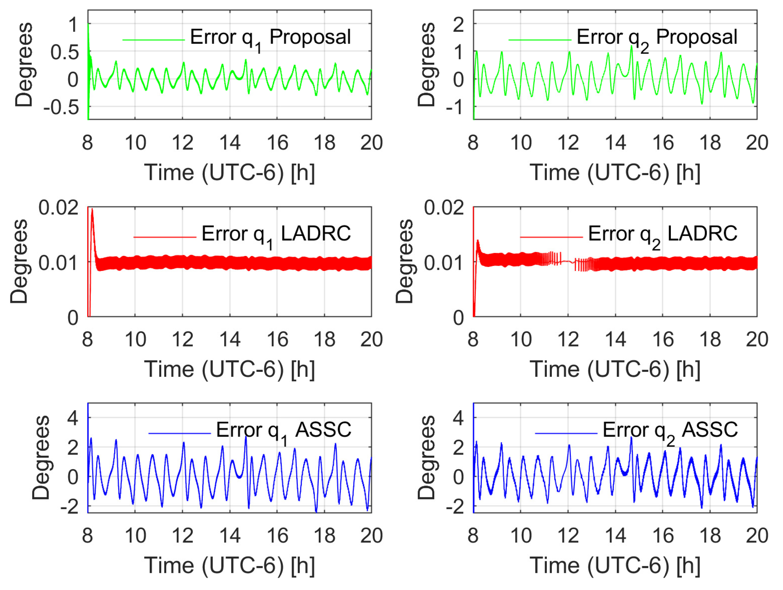
4.2. Numerical Results

To assess the behavior of the proposed controller, the trajectory tracking test was carried out in two conditions: without external disturbance and with a load on the end effector. Besides, in order to compare the results against reported active disturbance rejection controllers, two approaches were used for the test:

• A linear active disturbance rejection controller with an extended state observer was proposed [47];
• An adaptive active disturbance rejection control with disturbance approximation based on a linear state space combination (ASSC) [49].

Two different tests were carried out. The first test considered the robotic system without external disturbances, where the non-modeled dynamics were the only variable to compensate. The second test involved the application of a disturbance load of chaotic nature taken from the first state of a Chen system [58] with a normalization factor of $0.01$. The observer injection gains of the LADRC were set such that the linear dominant dynamics were of the form $(s^2+2{\zeta }_{ai}{\omega }_{ani}s+{\omega }_{ani}^2)(s+p_{ai})$, $i=1,2$ with ${\zeta }_{a1}={\zeta }_{a2}1$, ${\omega }_{an1}={\omega }_{an2}=14$, $p_{a1}=p_{a2}=0.5$, and the control gains of the LADRC were set to match the linear stable dynamics of the form $s^2+2{\zeta }_{aci}{\omega }_{acni}s+{\omega }_{acni}^2$, with ${\zeta }_{ac}={\zeta }_{ac2}=0.08$, ${\omega }_{acn1}={\omega }_{acn2}=120$. In the case of the ASSC, the same parameters as the proposal in both the controller and observer were used. Figure 3 shows the trajectory tracking error of the proposals for the unperturbed case. Notice that the LADRC achieves a smaller error but the adaptive proposals keep a competitive error bound in the context of solar tracking applications. Figure 4 depicts the effect of the disturbance in the controllers; in this case, the LADRC is shown to be more robust than the other schemes. However, this action demands a larger energy consumption, as shown in Figure 5, Figure 6, Figure 7 and Figure 8. The aggressive behavior of the control inputs in the LADRC, as shown in Figure 5 and Figure 6, implies larger amplitude values, in contrast with the proposal. Figure 7 and Figure 8 depict the energy consumption per actuator. Notice that the LADRC has around a five times larger consumption with respect to the proposal. The ASSC has a larger energy consumption (to a lesser extent) with respect to the proposal, which may be caused by the improvement in the generalized disturbance input. Finally, a cost function of the form

$$\begin{array}{c}\hfill J(x,\widehat{x})={\int }_0^t{\parallel \Delta \left(\tau \right)\parallel }^{2}d\tau \end{array}$$

is proposed to assess the quality of the state estimation by the observers. The behavior of the estimation error in the three cases denotes an ultimate bound behavior, which shows that the three strategies achieve good estimation results; in the case of the LADRC, it has the largest growing rate, which can be related to the high-gain nature, which has good results but some fluctuations that are accumulated in the integral term. Even so, the three schemes are, in general, good choices in the tracking task, and the proposal shows good estimation/tracking results and low energy consumption, and the LADRC shows the best robustness of the evaluated strategies. State estimation as Figure 9.

4.3. Experimental Results

Figure 10 shows the experimental robotic platform, whose parameters are listed in Table 1 and Figure 11 shows a general block diagram of the experimental platform including the user interface and the embedded system. The robotic system was actuated by means of two DC motors (Dongzen model 28JX20K139G/2838-1250S), with a nominal power of 2.9 W (12 V, 0.24 A), a geared transmission with a gear ratio of 1:139, and nominal torque of 9 Nm. The position sensors were incremental encoders with 1440 pulses per revolution. This information was sent to the microcontroller and decoded by means of two digital inputs implementing a gray code reading routine. The main control algorithm was programmed in a PC through the Waijung blockset simulink interface [59] and implemented through a STM32 Nucleo-F411RE microcontroller. The control law was implemented in the actuators by a PWM signal applied through a motor driver pololu model VNH5019. The numerical method used to implement the control was a fourth-order Runge–Kutta method with a sample time of 1 ms. In this case, the external disturbance $\eta \left(t\right)$ was due to the end effector consisting of a luminosity sensor with a nominal mass value of 0.12 Kg, which was not considered in the mathematical model, and the external wind load which presented variations from 0 to 12 Km/h according to the local weather report. Both signals were assumed as unknown external disturbances.

Figure 12 shows the tracking results for the azimuthal axis while Figure 13 shows the respective results for the elevation axis; the figures include the desired and actual trajectories and the error evolutions (with absolute bounds around 0.5 degrees). In order to assess the energy consumption with respect to the existing control approaches, a PID control was tuned such that it reached similar tracking results (see Figure 14 and Figure 15 to observe the tracking behavior); then, the energy consumption of the controllers was measured to evaluate if there was an energetic consumption advantage of the proposed controller. To measure the controller energy during the tracking task, an HER-423 Wattmeter was used for the complete cycle, with the following results: for the adaptive controller, the azimuthal axis expenditure was 95.35 Wh, and for the elevation angle, the expenditure was 94.68 Wh. That is, the total control consumption was 189.46 Wh. In the same test, the energy consumption of the PID control for the azimuthal axis was 104.65 Wh, and for the elevation axis, the energy consumption of the control actions was 105.88 Wh, leading to a total energy consumption of 210.53 Wh. That is, the proposal achieves about a $10\%$ energy saving with respect to a high-gain controller. Finally, Figure 16 and Figure 17 show the time varying behavior of the observer gains associated with the azimuthal and elevation axes.

From the numerical and experimental results, the following advantages and drawbacks of the strategy can be stated:

• As advantages, the proposal provides low energy consumption, achieving acceptable results in trajectory tracking for solar tracking. It showed low energy consumption with respect to both classic PID control and robust control of the LADRC nature. The adaptation rule is suitable for an implementation in embedded systems, which ensures low energy consumption in contrast with other strategies that are tested in a PC-based controller. The adaptive nature of the system may be suitable for noisy measurements with respect to high-gain state estimators.
• As possible drawbacks, even when the proposed tuning process is of the same nature as the classic PID and LADRC controllers, the process is not as natural as the former controllers. The robustness of the scheme is lower than that shown by the LADRC, but in the case of solar trackers, the mechanism design can contribute to avoiding aggressive robust actions. Besides, even when the system was successfully implemented in an embedded processor, the computational cost of the scheme was larger in comparison to classic schemes.

5. Conclusions

The proposed controller is a robust, low energy consuming alternative for trajectory tracking control in solar tracking systems, but the general structure allows this approach to be implemented in a general family of robotic systems modeled by Euler Lagrange equations. Besides, this approach respects the multivariable nature of the system, which is suitable for low gear ratio transmissions. Future implementations are planned for other robotic structures for solar tracking systems such as parallel configurations. On the other hand, the proposed class of controllers can be used for mobile robots which need low energetic cost controls in order to improve their global autonomy, enhancing the operation time.

References

1. Ohkubo, T.; Yabe, T.; Yoshida, K.; Uchida, S.; Funatsu, T.; Bagheri, B.; Oishi, T.; Daito, K.; Ishioka, M.; Nakayama, Y.; et al. Solar-pumped 80 W laser irradiated by a Fresnel lens. Opt. Lett. 2009, 34, 175–177. [Google Scholar] [CrossRef] [PubMed]
2. Allil, R.C.; Manchego, A.; Allil, A.; Rodrigues, I.; Werneck, A.; Diaz, G.C.; Dino, F.T.; Reyes, Y.; Werneck, M. Solar tracker development based on a POF bundle and Fresnel lens applied to environment illumination and microalgae cultivation. Sol. Energy 2018, 174, 648–659. [Google Scholar] [CrossRef]
3. Hidayanti, F.; Rahmah, F.; Agusto, J. Design of Solar Tracker on Solar Panel with Fresnel Concentrator. Int. J. Adv. Sci. Technol. 2020, 29, 1014–1025. [Google Scholar]
4. Bentaher, H.; Kaich, H.; Ayadi, N.; Hmouda, M.B.; Maalej, A.; Lemmer, U. A simple tracking system to monitor solar PV panels. Energy Convers. Manag. 2014, 78, 872–875. [Google Scholar] [CrossRef]
5. Camacho, E.; Berenguel, M.; Rubio, F.; Martínez, D. Control of Solar Energy Systems; Advances in Industrial Control b; Springer: London, UK, 2012. [Google Scholar]
6. Fernández-Ahumada, L.; Ramírez-Faz, J.; López-Luque, R.; Varo-Martínez, M.; Moreno-García, I.; de la Torre, F.C. Influence of the design variables of photovoltaic plants with two-axis solar tracking on the optimization of the tracking and backtracking trajectory. Sol. Energy 2020, 208, 89–100. [Google Scholar] [CrossRef]
7. Alexandru, C.; Irina Tatu, N. Optimal design of the solar tracker used for a photovoltaic string. J. Renew. Sustain. Energy 2013, 5, 023133. [Google Scholar] [CrossRef]
8. Alexandru, C. Optimal design of the dual-axis tracking system used for a PV string platform. J. Renew. Sustain. Energy 2019, 11, 043501. [Google Scholar] [CrossRef]
9. Al Garni, H.Z.; Awasthi, A.; Ramli, M.A. Optimal design and analysis of grid-connected photovoltaic under different tracking systems using HOMER. Energy Convers. Manag. 2018, 155, 42–57. [Google Scholar] [CrossRef]
10. Alexandru, C.; Pozna, C. Simulation of a dual-axis solar tracker for improving the performance of a photovoltaic panel. Proc. Inst. Mech. Eng. Part J. Power Energy 2010, 224, 797–811. [Google Scholar] [CrossRef]
11. Ahmed, R.; Oh, S.J.; Mehmood, M.U.; Kim, Y.; Jeon, G.; Han, H.J.; Lim, S.H. Computer vision and photosensor based hybrid control strategy for a two-axis solar tracker-Daylighting application. Sol. Energy 2021, 224, 175–183. [Google Scholar] [CrossRef]
12. Diaz, A.; Garrido, R.; Soto-Bernal, J. A filtered sun sensor for solar tracking in HCPV and CSP systems. IEEE Sens. J. 2018, 19, 917–925. [Google Scholar] [CrossRef]
13. Ortega, P.; López-Rodríguez, G.; Ricart, J.; Domínguez, M.; Castañer, L.M.; Quero, J.M.; Tarrida, C.L.; García, J.; Reina, M.; Gras, A.; et al. A miniaturized two axis sun sensor for attitude control of nano-satellites. IEEE Sens. J. 2010, 10, 1623–1632. [Google Scholar] [CrossRef] [Green Version]
14. Saymbetov, A.; Mekhilef, S.; Kuttybay, N.; Nurgaliyev, M.; Tukymbekov, D.; Meiirkhanov, A.; Dosymbetova, G.; Svanbayev, Y. Dual-axis schedule tracker with an adaptive algorithm for a strong scattering of sunbeam. Sol. Energy 2021, 224, 285–297. [Google Scholar] [CrossRef]
15. Urbano, J.A.; Matsumoto, Y.; Asomoza, R.; Aceves, F.; Sotelo, A.; Jacome, A. 5 Wp PV module-based stand-alone solar tracking system. In Proceedings of the 3rd World Conference on Photovoltaic Energy Conversion, Osaka, Japan, 11–18 May 2003; Volume 3, pp. 2463–2465. [Google Scholar]
16. Lee, C.Y.; Chou, P.C.; Chiang, C.M.; Lin, C.F. Sun tracking systems: A review. Sensors 2009, 9, 3875–3890. [Google Scholar] [CrossRef]
17. Nsengiyumva, W.; Chen, S.G.; Hu, L.; Chen, X. Recent advancements and challenges in Solar Tracking Systems (STS): A review. Renew. Sustain. Energy Rev. 2018, 81, 250–279. [Google Scholar] [CrossRef]
18. Hafez, A.; Yousef, A.; Harag, N. Solar tracking systems: Technologies and trackers drive types—A review. Renew. Sustain. Energy Rev. 2018, 91, 754–782. [Google Scholar] [CrossRef]
19. Sumathi, V.; Jayapragash, R.; Bakshi, A.; Akella, P.K. Solar tracking methods to maximize PV system output—A review of the methods adopted in recent decade. Renew. Sustain. Energy Rev. 2017, 74, 130–138. [Google Scholar] [CrossRef]
20. Barbón, A.; Bayón-Cueli, C.; Bayón, L.; Ayuso, P.F. Influence of solar tracking error on the performance of a small-scale linear Fresnel reflector. Renew. Energy 2020, 162, 43–54. [Google Scholar] [CrossRef]
21. Fuentes-Morales, R.F.; Diaz-Ponce, A.; Peña-Cruz, M.I.; Rodrigo, P.M.; Valentín-Coronado, L.M.; Martell-Chavez, F.; Pineda-Arellano, C.A. Control algorithms applied to active solar tracking systems: A review. Sol. Energy 2020, 212, 203–219. [Google Scholar] [CrossRef]
22. Sidek, M.; Azis, N.; Hasan, W.; Ab Kadir, M.; Shafie, S.; Radzi, M. Automated positioning dual-axis solar tracking system with precision elevation and azimuth angle control. Energy 2017, 124, 160–170. [Google Scholar] [CrossRef]
23. Sabir, M.M.; Ali, T. Optimal PID controller design through swarm intelligence algorithms for sun tracking system. Appl. Math. Comput. 2016, 274, 690–699. [Google Scholar] [CrossRef]
24. Spong, M.; Hutchinson, S.; Vidyasagar, M. Robot Modeling and Control; John Wiley: Hoboken, NJ, USA, 2006. [Google Scholar]
25. Visioli, A. Practical PID Control; Springer Science & Business Media: Berlin/Heidelberg, Germany, 2006. [Google Scholar]
26. Shamsuzzoha, M.; Skogestad, S. The setpoint overshoot method: A simple and fast closed-loop approach for PID tuning. J. Process. Control 2010, 20, 1220–1234. [Google Scholar] [CrossRef]
27. Ali, A.; Majhi, S. PI/PID controller design based on IMC and percentage overshoot specification to controller setpoint change. ISA Trans. 2009, 48, 10–15. [Google Scholar] [CrossRef] [PubMed]
28. Li, K.; Boonto, S.; Nuchkrua, T. On-line self tuning of contouring control for high accuracy robot manipulators under various operations. Int. J. Control Autom. Syst. 2020, 18, 1818–1828. [Google Scholar] [CrossRef]
29. Nuchkrua, T.; Leephakpreeda, T. Fuzzy self-tuning PID control of hydrogen-driven pneumatic artificial muscle actuator. J. Bionic Eng. 2013, 10, 329–340. [Google Scholar] [CrossRef]
30. Roman, R.C.; Precup, R.E.; Petriu, E.M. Hybrid data-driven fuzzy active disturbance rejection control for tower crane systems. Eur. J. Control 2021, 58, 373–387. [Google Scholar] [CrossRef]
31. Hou, Z.; Xiong, S. On model-free adaptive control and its stability analysis. IEEE Trans. Autom. Control 2019, 64, 4555–4569. [Google Scholar] [CrossRef]
32. Safan, Y.M.; Shaaban, S.; El-Sebah, M.I.A. Performance evaluation of a multi-degree of freedom hybrid controlled dual axis solar tracking system. Sol. Energy 2018, 170, 576–585. [Google Scholar] [CrossRef]
33. Lashab, A.; Sera, D.; Guerrero, J.M.; Máthé, L.; Bouzid, A. Discrete model-predictive-control-based maximum power point tracking for PV systems: Overview and evaluation. IEEE Trans. Power Electron. 2017, 33, 7273–7287. [Google Scholar] [CrossRef]
34. Rubio, F.; Ortega, M.; Gordillo, F.; Lopez-Martinez, M. Application of new control strategy for sun tracking. Energy Convers. Manag. 2007, 48, 2174–2184. [Google Scholar] [CrossRef]
35. Kim, I.S. Robust maximum power point tracker using sliding mode controller for the three-phase grid-connected photovoltaic system. Sol. Energy 2007, 81, 405–414. [Google Scholar] [CrossRef]
36. Chu, C.C.; Chen, C.L. Robust maximum power point tracking method for photovoltaic cells: A sliding mode control approach. Sol. Energy 2009, 83, 1370–1378. [Google Scholar] [CrossRef]
37. Alata, M.; Al-Nimr, M.; Qaroush, Y. Developing a multipurpose sun tracking system using fuzzy control. Energy Convers. Manag. 2005, 46, 1229–1245. [Google Scholar] [CrossRef]
38. Al Nabulsi, A.; Dhaouadi, R. Efficiency optimization of a DSP-based standalone PV system using fuzzy logic and dual-MPPT control. IEEE Trans. Ind. Inform. 2012, 8, 573–584. [Google Scholar] [CrossRef]
39. Bahgat, A.; Helwa, N.; Ahmad, G.; El Shenawy, E. Maximum power point traking controller for PV systems using neural networks. Renew. Energy 2005, 30, 1257–1268. [Google Scholar] [CrossRef]
40. AL-Rousan, N.A.; Isa, N.A.M.; Desa, M.K.M. Efficient Single and Dual Axis Solar Tracking System Controllers Based on Adaptive Neural Fuzzy Inference System. J. King Saud-Univ.-Eng. Sci. 2020, 32, 459–469. [Google Scholar] [CrossRef]
41. Han, J. From PID to active disturbance rejection control. IEEE Trans. Ind. Electron. 2009, 56, 900–906. [Google Scholar] [CrossRef]
42. Gao, Z. Active disturbance rejection control: A paradigm shift in feedback control system design. In Proceedings of the American Control Conference, Minneapolis, MN, USA, 14–16 June 2006; IEEE: New York, NY, USA, 2006; pp. 2399–2405. [Google Scholar]
43. Chu, Z.; Wu, C.; Sepehri, N. Active disturbance rejection control applied to high-order systems with parametric uncertainties. Int. J. Control. Autom. Syst. 2019, 17, 1483–1493. [Google Scholar] [CrossRef]
44. Liu, F.; Li, H.; Liu, L.; Zou, R.; Liu, K. A Control Method for IPMSM Based on Active Disturbance Rejection Control and Model Predictive Control. Mathematics 2021, 9, 760. [Google Scholar] [CrossRef]
45. Patelski, R.; Dutkiewicz, P. On the stability of ADRC for manipulators with modelling uncertainties. ISA Trans. 2020, 102, 295–303. [Google Scholar] [CrossRef]
46. Madoński, R.; Herman, P. Survey on methods of increasing the efficiency of extended state disturbance observers. ISA Trans. 2015, 56, 18–27. [Google Scholar] [CrossRef]
47. Sira-Ramírez, H.; Luviano-Juárez, A.; Ramírez-Neria, M.; Zurita-Bustamante, E.W. Active Disturbance Rejection Control of Dynamic Systems: A Flatness Based Approach; Butterworth-Heinemann: Oxford, UK, 2017. [Google Scholar]
48. Ahi, B.; Haeri, M. Linear active disturbance rejection control from the practical aspects. IEEE/ASME Trans. Mechatron. 2018, 23, 2909–2919. [Google Scholar] [CrossRef]
49. Lozada-Castillo, N.; Luviano-Juárez, A.; Chairez, I. Robust control of uncertain feedback linearizable systems based on adaptive disturbance estimation. ISA Trans. 2019, 87, 1–9. [Google Scholar] [CrossRef]
50. Nuchkrua, T.; Leephakpreeda, T. Novel Compliant Control of Pneumatic Artificial Muscle Driven by Hydrogen Pressure under Varying Environment. IEEE Trans. Ind. Electron. 2021. [Google Scholar] [CrossRef]
51. Escobar, J.; Poznyak, A. Time-varying matrix estimation in stochastic continuous-time models under coloured noise using LSM with forgetting factor. Int. J. Syst. Sci. 2011, 42, 2009–2020. [Google Scholar] [CrossRef]
52. Poznyak, A. Advanced Mathematical Tools for Control Engineers: Volume 1: Deterministic Systems; Elsevier: Amsterdam, The Netherlands, 2010. [Google Scholar]
53. Horn, R.; Johnson, C. Matrix Analysis; Cambridge University Press: Cambridge, UK, 2012. [Google Scholar]
54. Khalil, H. Nonlinear Systems; Prentice Hall: Upper Saddle River, NJ, USA, 2002. [Google Scholar]
55. Flores-Hernandez, D.; Palomino-Resendiz, S.; Luviano-Juárez, A.; Lozada-Castillo, N.; Gutierrez-Frias, O. A heuristic approach for tracking error and energy consumption minimization in solar tracking systems. IEEE Access 2019, 7, 52755–52768. [Google Scholar] [CrossRef]
56. Cooper, P. The absorption of radiation in solar stills. Sol. Energy 1969, 12, 333–346. [Google Scholar] [CrossRef]
57. da Silva Campos, V.C.; Nguyen, A.T.; Palhares, R.M. Adaptive gain-scheduling control for continuous-time systems with polytopic uncertainties: An LMI-based approach. Automatica 2021, 133, 109856. [Google Scholar] [CrossRef]
58. Sira-Ramirez, H.; Fliess, M. An algebraic state estimation approach for the recovery of chaotically encrypted messages. Int. J. Bifurc. Chaos 2006, 16, 295–309. [Google Scholar] [CrossRef]
59. Hmidet, A.; Hasnaoui, O. Waijung blockset-STM32F4 environment for real time induction motor speed control. In Proceedings of the 2018 IEEE 5th International Congress on Information Science and Technology (CiSt), Marrakech, Morocco, 21–27 October 2018; IEEE: New York, NY, USA, 2018; pp. 600–605. [Google Scholar]
Figure 1. Schematic of the proposed adaptive active disturbance rejection controller.
Mathematics 09 02871 g001
Figure 2. Schematic of the robotic system.
Mathematics 09 02871 g002
Figure 3. Tracking error behavior comparison (non-disturbed case) for azimuthal axis ( q 1 ) and elevation axis ( q 2 ). LADRC stands for linear active disturbance rejection control and ASSC for adaptive state space combination.
Mathematics 09 02871 g003
Figure 4. Tracking error behavior comparison (disturbed case) for azimuthal axis ( q 1 ) and elevation axis ( q 2 ). LADRC stands for linear active disturbance rejection control and ASSC for adaptive state space combination.
Mathematics 09 02871 g004
Figure 5. Control input behavior comparison (non-disturbed case).
Mathematics 09 02871 g005
Figure 6. Control input behavior comparison (disturbed case).
Mathematics 09 02871 g006
Figure 7. Energy consumption per actuator (unperturbed case).
Mathematics 09 02871 g007
Figure 8. Energy consumption per actuator (perturbed case).
Mathematics 09 02871 g008
Figure 9. Performance index behavior of the state estimation. The graphics on the left side denote the case without disturbance and the graphics on the right side show the performance in presence of disturbance.
Mathematics 09 02871 g009
Figure 10. Experimental test bed of the solar tracking system.
Mathematics 09 02871 g010
Figure 11. Block diagram of the experimental robotic system.
Mathematics 09 02871 g011
Figure 12. Tracking behavior for the azimuthal axis.
Mathematics 09 02871 g012
Figure 13. Tracking behavior for the elevation axis.
Mathematics 09 02871 g013
Figure 14. Tracking behavior for the azimuthal axis (PID control).
Mathematics 09 02871 g014
Figure 15. Tracking behavior for the elevation axis (PID control).
Mathematics 09 02871 g015
Figure 16. Observer gain behavior for the azimuthal axis injection.
Mathematics 09 02871 g016
Figure 17. Observer gain behavior for the elevation axis injection.
Mathematics 09 02871 g017