Adaptation of Residual-Error Series Algorithm to Handle Fractional System of Partial Differential Equations

Abstract

In this article, an attractive numeric–analytic algorithm, called the fractional residual power series algorithm, is implemented for predicting the approximate solutions for a certain class of fractional systems of partial differential equations in terms of Caputo fractional differentiability. The solution methodology combines the residual function and the fractional Taylor’s formula. In this context, the proposed algorithm provides the unknown coefficients of the expansion series for the governed system by a straightforward pattern as well as it presents the solutions in a systematic manner without including any restrictive conditions. To enhance the theoretical framework, some numerical examples are tested and discussed to detect the simplicity, performance, and applicability of the proposed algorithm. Numerical simulations and graphical plots are provided to check the impact of the fractional order on the geometric behavior of the fractional residual power series solutions. Moreover, the efficiency of this algorithm is discussed by comparing the obtained results with other existing methods such as Laplace Adomian decomposition and Iterative methods. Simulation of the results shows that the fractional residual power series technique is an accurate and very attractive tool to obtain the solutions for nonlinear fractional partial differential equations that occur in applied mathematics, physics, and engineering.

1. Introduction

Fractional partial differential equations (FPDEs) play a substantial role in converting several physical systems into mathematical models. It is normally advised to utilize this formula to keep historical cases of the original systems, in addition to its behavior. Indeed, this will aid in attaining a superior comprehension of those physical systems, decrease computational complexity, and moderate the controller designing without losing any hereditary behaviors. In the last few decades, FPDEs have gained considerable attention because they are popularly utilized to explain many complex phenomena in different applications such as signal processing, information theory, control theory, finance, fluid flow, and systems identification [1,2,3,4]. The fractional derivatives are superb tools for the depiction of hereditary and memory properties of different engineering, mathematical, and physical problems.

Obtaining explicit and approximate solutions for FPDEs is a difficult task. So, various numerical and analytical techniques have been developed to investigate the solutions for the systems of FPDEs, such as the Adomian decomposition technique, homotopy perturbation technique, variational iteration technique, reproducing kernel technique, and homotopy perturbation transform technique [5,6,7,8,9]. For more information regarding the methods and numerical techniques for solving fractional differential equations, see [10,11,12,13,14].

The main purpose of this work is to construct the solutions for a certain class of linear and non-linear systems of FPDEs under the name Caputo derivative by using a promising numeric–analytic technique, called a fractional residual power series (FRPS) method, see [15,16] and the references therein. The present method is based mainly on the generalized Taylor’s series and the residual error concept where the solution of the original equation is provided as an expanded fractional power series via finding the unknown coefficients of the proposed series formula by recurrent Caputo fractional derivative of the truncated residual functions. Recent years have witnessed extended applications of the fractional RPS technique, including the fractional Newell–Whitehead–Segel equation [15], fractional stiff system [16], fractional Sawada–Kotera–Ito, Lax, and Kaup–Kupershmidt equations [17], time-fractional Fokker–Planck equations [18], the fractional Kundu–Eckhaus and massive Thirring models [19], coupled fractional resonant Schrödinger equation [20], and fractional Sharma–Tasso–Olever equation [21]. The fractional RPS algorithm is a straightforward, applicable, and powerful approach to create fractional power series (FPS) solutions for strongly linear and non-linear equations without terms of perturbation, discretization, and linearization [22,23,24,25,26,27,28,29]. Series expansions are very useful tools in numerical simulations, especially for quick estimates made in manual arithmetic, and in evaluating functions, integrals, and derivatives. Since the advent of modern computational technology, it has become common practice to deal directly with PDEs numerically, using various simulations rather than series expansions. However, in terms of developing analytic methods for multidimensional mathematical formula and finding exact and approximate solutions, one should expect a renewed interest in series expansions. In view of the residual error functions, the main advantage of this RPS algorithm enables the simplicity of computing coefficients within imposed conditions using only differential operators by using the Mathematica software package, unlike other analytical methods that require integral operators which are difficult in the fractional sense. It is not affected by round arithmetic errors and can also be implemented without any restrictions on the nature of the system and the type of classification.

Great attention has been paid to fractional partial differential equations due to their vital role of the exact description of both linear and nonlinear mathematical problems. When analyzing a mathematical model that represents some physical phenomena, such as the current model, especially the nonlinear system of PDEs, the motivation of mathematicians is to find a solution to such a system and to study the stability and singularities for long periods of time: the dynamics and physical properties, and the transfer of energy between waves propagating within a phase plan, and the constraints that have to be imposed on the system parameters to obtain waves of different frequencies. Motivated by the above discussion, we intend in this work to design a rigorous algorithm capable of building a straightforward and effective method for finding analytical solutions for these systems. Accordingly, the main contribution is the creation of a new algorithm and the finding of accurate and efficient approximate solutions to a system of fractional order partial differential equations within the framework of the Caputo concept in the field of interest.

The structure of this work is arranged as follows: in the next section, some substantial definitions and their properties related to fractional calculus are revisited and primary remarks of generalized Taylor’s series are provided. In Section 3, the fractional RPS algorithm is introduced to create the approximate solutions for a non-linear system of FPDEs. In Section 4, two linear and non-linear systems of FPDEs are tested to illustrate the simplicity and potentiality of the fractional RPS approach for determining the approximate solutions. In Section 5, the obtained results are discussed graphically and numerically. Finally, a short conclusion is made in the last section.

2. Basic Concepts and Notations

Various definitions for integrals and derivatives of fractional order have been proposed and developed in the literature. The most popular of these definitions are Riemann-Liouville’s definition, Riesz’s definition, Caputo’s definition, and Grunwald–Letnikov’s definition. Many researchers [3,4,5,6] prefer employing the Caputo operator, due to the initial data for the FPDEs which can be achieved with a similar utilization of the ordinal case. This section is devoted to review the essential definitions and primary results concerned with the integrals and derivatives of fractional order. As well, we revise the notable results of the generalized Taylor’s series, which will be used in the next sections.

Definition 1.

For $\alpha \in {ℝ}^{+}$, the Riemann–Liouville fractional integral operator for a real-valued function$\mathsf{ⱳ}\left(x,t\right)$is denoted by${\mathcal{J}}_t^{\alpha }$and defined as [3]:

$${\mathcal{J}}_t^{\alpha }\mathsf{ⱳ}\left(x,t\right)=\left\{\begin{array}{ll}\frac{1}{\Gamma \left(\alpha \right)}\underset{0}{\overset{t}{{\displaystyle \int }}}\frac{\mathsf{ⱳ}\left(x,\eta \right)}{{\left(t-\eta \right)}^{1-\alpha }}d\eta , \hfill & 0<\eta <t,\alpha >0\hfill \\ \mathsf{ⱳ}\left(x,t\right)\hfill & \alpha =0\hfill \end{array}\right.$$

Thus, for ${\alpha }_1, {\alpha }_2>0$, and $\beta >-1$, the operator ${\mathcal{J}}_t^{\alpha }$ satisfy the following properties:

• ${\mathcal{J}}_t^{\alpha }c=\frac{c}{\Gamma \left(\alpha +1\right)}{\left(t-\eta \right)}^{\alpha }$, $c\in ℝ$.
• ${\mathcal{J}}_t^{{\alpha }_1}{\mathcal{J}}_t^{{\alpha }_2}\mathsf{ⱳ}\left(x,t\right)={\mathcal{J}}_t^{{\alpha }_1+, {\alpha }_2}\mathsf{ⱳ}\left(x,t\right)={\mathcal{J}}_t^{{\alpha }_2}{\mathcal{J}}_t^{{\alpha }_1}\mathsf{ⱳ}\left(x,t\right)$.
• ${\mathcal{J}}_t^{\alpha }{\left(t-\eta \right)}^{\beta }=\frac{\Gamma \left(\beta +1\right)}{\Gamma \left(\beta +\alpha +1\right)}{\left(t-\eta \right)}^{\beta +\alpha }$.

Definition 2.

The time fractional derivative of order$\alpha >0$, for the function  $\mathsf{ⱳ}\left(x,t\right)$ in the Caputo case is denoted by$\frac{{\partial }^{\alpha }}{\partial t^{\alpha }}$, and is defined as [3]:

$$\frac{{\partial }^{\alpha }}{\partial t^{\alpha }}\mathsf{ⱳ}\left(x,t\right)=\left\{\begin{array}{ll}{\mathcal{J}}_t^{n-\alpha }\left(\frac{{\partial }^n}{\partial t^n}\mathsf{ⱳ}\left(x,t\right)\right),\hfill & 0<n-1<\alpha \le n ,\hfill \\ \frac{{\partial }^n}{\partial t^n}\mathsf{ⱳ}\left(x,t\right),\hfill & \alpha =n, n\in \mathbb{N}.\hfill \end{array}\right.$$

Lemma 1.

For $n-1<\alpha \le n, \rho >n-1, n\in \mathbb{N}, \rho \in ℝ$, the operator $\frac{{\partial }^{\alpha }}{\partial t^{\alpha }}$ satisfies the following properties [12]:

(1)

$\frac{{\partial }^{\alpha }}{\partial t^{\alpha }}c=0$, $c\in ℝ$.

(2)

$\frac{{\partial }^{\alpha }}{\partial t^{\alpha }}{\left(t-\eta \right)}^{\rho }=\frac{\Gamma \left(\rho +1\right)}{\Gamma \left(\rho +1-\alpha \right)}{\left(t-\eta \right)}^{\rho -\alpha }$.

(3)

${\mathcal{J}}_t^{\alpha }\frac{{\partial }^{\alpha }}{\partial t^{\alpha }}\mathsf{ⱳ}\left(x,t\right)=\mathsf{ⱳ}\left(x,t\right)-{\displaystyle \sum }_{j=0}^{n-1}\frac{{\partial }^j}{\partial x^j}\left(x,\eta \right)\frac{{\left(t-\eta \right)}^j}{j!}$, for$\mathsf{ⱳ}\left(x,t\right)\in C^n\left[a,b\right]$.

(4)

${\mathcal{J}}_t^{\alpha }\frac{{\partial }^{\alpha }}{\partial t^{\alpha }}\mathsf{ⱳ}\left(x,t\right)=\mathsf{ⱳ}\left(x,t\right)$, for$\mathsf{ⱳ}\left(x,t\right)\in C\left[a,b\right]$.

Definition 3.

A fractional expansion representation at $t=\eta$has the following form:

$${\displaystyle \sum }_{k=0}^{\infty }{\mathsf{ⱳ}}_k\left(x\right)\left(t-\eta \right){ }^{\alpha k}={\mathsf{ⱳ}}_0\left(x\right)+{\mathsf{ⱳ}}_1\left(x\right){\left(t-\eta \right)}^{\alpha }+{\mathsf{ⱳ}}_2\left(x\right){\left(t-\eta \right)}^{2\alpha }+\dots$$

where$0\le n-1<\alpha \le n$,$x\in I$and$t\ge \eta$is called multiple fractional power series (MFPS) about$\eta$ [15].

Theorem 1.

Suppose that $\mathsf{ⱳ}\left(x,t\right)$has the following MFPS representation at $t=\eta$:

$$\mathsf{ⱳ}\left(x,t\right)={\displaystyle \sum }_{k=0}^{\infty }{\mathsf{ⱳ}}_k\left(x\right)\left(t-\eta \right){ }^{\alpha k}, 0\le n-1<\alpha \le n , x\in I,t\in \left[ \eta ,\eta +R\right).$$

where$\mathsf{ⱳ}\left(x,t\right)\in C\left(I\times \left[\eta ,\eta +R^{1/\alpha } \right)\right)$and$\frac{{\partial }^{\left(k-1\right)\alpha }}{\partial t^{\left(k-1\right)\alpha }}\mathsf{ⱳ}\left(x,t\right)\in C\left(I\times \left[\eta ,\eta +R^{1/\alpha } \right)\right)$,$k=1,2,\dots$, and$\frac{{\partial }^{\left(m-1\right)\alpha }}{\partial t^{\left(m-1\right)\alpha }}\left(\frac{{\partial }^{\left(k-1\right)\alpha }}{\partial t^{\left(k-1\right)\alpha }}\mathsf{ⱳ}\left(x,t\right)\right)$is well defined on$\left(\eta ,\eta +R^{1/\alpha }\right)$for$m=2,\dots ,n-1,$and$k=1,2,\dots$, then the unknown functions${\mathsf{ⱳ}}_k\left(x\right)$will be in the form${\mathsf{ⱳ}}_k\left(x\right)=\frac{1}{\Gamma \left(k\alpha +1\right)}\frac{{\partial }^{k\alpha }\mathsf{ⱳ}\left(x,\eta \right)}{\partial t^{k\alpha }}$, such that$\frac{{\partial }^{k\alpha }}{\partial t^{k\alpha }}=\frac{{\partial }^{\alpha }}{\partial t^{\alpha }}\mathsf{ⱳ}\frac{{\partial }^{\alpha }}{\partial t^{\alpha }}\mathsf{ⱳ}\mathsf{ⱳ}\mathsf{ⱳ}\frac{{\partial }^{\alpha }}{\partial t^{\alpha }},$k-times [15].

Proof. 

Assuming that $\mathsf{ⱳ}\left(x,t\right)={\mathsf{ⱳ}}_0\left(x\right)+{\mathsf{ⱳ}}_1\left(x\right){\left(t-\eta \right)}^{\alpha }+{\mathsf{ⱳ}}_2\left(x\right){\left(t-\eta \right)}^{2\alpha }+\dots ,$$t_0\le t<\eta +R^{1/\alpha },$ then directly ${\mathsf{ⱳ}}_0\left(x\right)=\mathsf{ⱳ}\left(x,\eta \right).$ By applying $\frac{{\partial }^{\alpha }}{\partial t^{\alpha }}$ to $\mathsf{ⱳ}\left(x,t\right)$ and evaluating the result at $\eta$, it yields that $\frac{{\partial }^{\alpha }}{\partial t^{\alpha }}\mathsf{ⱳ}\left(x,\eta \right)=\Gamma \left(\alpha +1\right){\mathsf{ⱳ}}_1\left(x\right)$ and hence ${\mathsf{ⱳ}}_1\left(x\right)=\frac{\frac{{\partial }^{\alpha }}{\partial t^{\alpha }}\mathsf{ⱳ}\left(x,\eta \right)}{\Gamma \left(\alpha +1\right)}.$ Proceeding inductively and applying $\frac{{\partial }^{k\alpha }}{\partial t^{k\alpha }}$ to $\mathsf{ⱳ}\left(x,t\right)$$k$-times and evaluating the result at $\eta$, one can note that $\frac{{\partial }^{k\alpha }}{\partial t^{k\alpha }}\mathsf{ⱳ}\left(x,\eta \right)=\Gamma \left(k\alpha +1\right){\mathsf{ⱳ}}_k\left(x\right)$ and hence the proof is completed. □

3. FRPS Technique

Fractional RPS technique provides solutions for some related physical phenomena in the form of fractional power series. In the present section, the basic principle of the FRPS technique for solving a system of linear and non-linear FPDEs is introduced. Our strategy to use the proposed scheme depends on employing the fractional Taylor’s series based on the meaning of the Caputo fractional derivative and the concept of residual function. More specifically, we consider the following initial value problems for a system of FPDEs:

$$\begin{gathered} \frac{{\partial }^{\alpha }\mathsf{ⱳ}}{\partial t^{\alpha }}+{\mathcal{R}}_1\left(\mathsf{ⱳ},\phi \right)+{\mathcal{N}}_1\left(\mathsf{ⱳ},\phi \right)=f\left(x,t\right), \\ \frac{{\partial }^{\alpha }\phi }{\partial t^{\alpha }}+{\mathcal{R}}_2\left(\mathsf{ⱳ},\phi \right)+{\mathcal{N}}_2\left(\mathsf{ⱳ},\phi \right)=g\left(x,t\right), \end{gathered}$$

(1)

subject to initial conditions

$$\mathsf{ⱳ}\left(x,0\right)=\mathsf{ⱳ}\left(x\right) \mathrm{and} \phi \left(x,0\right)=\phi \left(x\right).$$

(2)

where $t\ge 0$, $x\in ℝ$, $\frac{{\partial }^{\alpha }}{\partial t^{\alpha }}$ refers to $\alpha$-th Caputo fractional derivative for $\alpha \in \left(0,1\right]$, $\mathsf{ⱳ}\left(x,t\right)$, $\phi \left(x,t\right)$ are two unknown functions to be determined, and ${\mathcal{R}}_1, {\mathcal{R}}_2, {\mathcal{N}}_1$, and ${\mathcal{N}}_2$ are linear and non-linear operators, respectively, and $f$, $g$ are two continuous functions. In this analysis, we assume that $\mathsf{ⱳ}\left(x,t\right),$ and $\phi \left(x,t\right)$ satisfy the requirements for the existence of a unique solution and satisfies all conditions to have a MFPS representation at $t=0$.

Now, the methodology of the proposed scheme consists of assuming that the solutions of the system (1) and (2) have a MFPS as follows:

$$\begin{gathered} \mathsf{ⱳ}\left(x,t\right)={\displaystyle \sum }_{n=0}^{\infty }{\mathsf{ⱳ}}_n\left(x\right)t^{\alpha n}, 0\le t<R, x\in ℝ, \alpha \in \left(0,1\right], \\ \phi \left(x,t\right)={\displaystyle \sum }_{n=0}^{\infty }{\phi }_n\left(x\right)t^{\alpha n}, 0\le t<R, x\in ℝ, \alpha \in \left(0,1\right]. \end{gathered}$$

(3)

Evidently, the assumed solutions (3) satisfy the initial conditions (2), so from (3), one can get $\mathsf{ⱳ}\left(x,0\right)={\mathsf{ⱳ}}_0\left(x\right)=\mathsf{ⱳ}\left(x\right)$, and $\phi \left(x,0\right)={\phi }_0\left(x\right)=\phi \left(x\right)$. Hence, the expansions in (3) can be reformulated into the following shape:

$$\begin{gathered} \mathsf{ⱳ}\left(x,t\right)=\mathsf{ⱳ}\left(x\right)+{\displaystyle \sum }_{n=1}^{\infty }{\mathsf{ⱳ}}_n\left(x\right)t^{\alpha n}, 0\le t<R, x\in ℝ, \alpha \in \left(0,1\right], \\ \phi \left(x,t\right)=\phi \left(x\right)+{\displaystyle \sum }_{n=1}^{\infty }{\phi }_n\left(x\right)t^{\alpha n}, 0\le t<R, x\in ℝ, \alpha \in \left(0,1\right]. \end{gathered}$$

Next, one can approximate the series solutions by the following $j$-th truncation series:

$$\begin{gathered} {\mathsf{ⱳ}}_j\left(x,t\right)=\mathsf{ⱳ}\left(x\right)+{\displaystyle \sum }_{n=1}^j{\mathsf{ⱳ}}_n\left(x\right)t^{\alpha n}, 0\le t<R, x\in ℝ, \alpha \in \left(0,1\right], \\ {\phi }_j\left(x,t\right)=\phi \left(x\right)+{\displaystyle \sum }_{n=1}^j{\phi }_n\left(x\right)t^{\alpha n}, 0\le t<R, x\in ℝ, \alpha \in \left(0,1\right]. \end{gathered}$$

(4)

As stated in [16,17,18,19], we can obtain the unknown functions ${\mathsf{ⱳ}}_n\left(x\right)$, and ${\phi }_n\left(x\right)$, for $n=1,2,\dots ,j$, throughout by solving the following fractional algebraic equations for $j=1,2,\dots$ and $0<\alpha \le 1$:

$$\begin{gathered} \frac{{\partial }^{\left(j-1\right)\alpha }}{\partial t^{\left(j-1\right)\alpha }}Re{s}_{\mathsf{ⱳ}}^j\left(x,0\right)=0, \\ \frac{{\partial }^{\left(j-1\right)\alpha }}{\partial t^{\left(j-1\right)\alpha }}Re{s}_{\phi }^j\left(x,0\right)=0. \end{gathered}$$

(5)

where $Re{s}_{\mathsf{ⱳ}}^j$ and $Re{s}_{\phi }^j$ are called the $j$-th residual functions that are defined as:

$$\begin{gathered} Re{s}_{\mathsf{ⱳ}}^j\left(x,t\right)=\frac{{\partial }^{\alpha }{\mathsf{ⱳ}}_j\left(x,t\right)}{\partial t^{\alpha }}+{\mathcal{R}}_1\left({\mathsf{ⱳ}}_j\left(x,t\right),{\phi }_j\left(x,t\right)\right)+{\mathcal{N}}_1\left({\mathsf{ⱳ}}_j\left(x,t\right),{\phi }_j\left(x,t\right)\right)-f\left(x,t\right), \\ Re{s}_{\phi }^j\left(x,t\right)=\frac{{\partial }^{\alpha }{\phi }_j\left(x,t\right)}{\partial t^{\alpha }}+{\mathcal{R}}_2\left({\mathsf{ⱳ}}_j\left(x,t\right),{\phi }_j\left(x,t\right)\right)+{\mathcal{N}}_2\left({\mathsf{ⱳ}}_j\left(x,t\right),{\phi }_j\left(x,t\right)\right)-g\left(x,t\right), \end{gathered}$$

(6)

whereas $Re{s}_{\mathsf{ⱳ}}$ and $Re{s}_{\phi }$ are given as:

$$\begin{gathered} Re{s}_{\mathsf{ⱳ}}\left(x,t\right)=\underset{j\to \infty }{\lim }Re{s}_{\mathsf{ⱳ}}^j\left(x,t\right) \\ =\frac{{\partial }^{\alpha }\mathsf{ⱳ}\left(x,t\right)}{\partial t^{\alpha }}+{\mathcal{R}}_1\left(\mathsf{ⱳ}\left(x,t\right),\phi \left(x,t\right)\right)+{\mathcal{N}}_1\left(\mathsf{ⱳ}\left(x,t\right),\phi \left(x,t\right)\right)-f\left(x,t\right), \\ Re{s}_{\phi }\left(x,t\right)=\underset{j\to \infty }{\lim }Re{s}_{\phi }^j\left(x,t\right) \\ =\frac{{\partial }^{\alpha }\phi \left(x,t\right)}{\partial t^{\alpha }}+{\mathcal{R}}_2\left(\mathsf{ⱳ}\left(x,t\right),\phi \left(x,t\right)\right)+{\mathcal{N}}_2\left(\mathsf{ⱳ}\left(x,t\right),\phi \left(x,t\right)\right)-g\left(x,t\right). \end{gathered}$$

There are some useful results of the residual functions which are basic to our scheme and can be listed as:

• $Re{s}_{\mathsf{ⱳ}}\left(x,t\right)=0$, and $Re{s}_{\phi }\left(x,t\right)=0$.
• $\underset{j\to \infty }{\lim }Re{s}_{\mathsf{ⱳ}}^j\left(x,t\right)=Re{s}_{\mathsf{ⱳ}}\left(x,t\right)$, and $\underset{j\to \infty }{\lim }Re{s}_{\phi }^j\left(x,t\right)=Re{s}_{\phi }\left(x,t\right)$, for each $0\le t, x\in ℝ$.
• $\frac{{\partial }^{\left(k-1\right)\alpha }}{\partial t^{\left(k-1\right)\alpha }}Re{s}_{\mathsf{ⱳ}}\left(x,0\right)=\frac{{\partial }^{\left(k-1\right)\alpha }}{\partial t^{\left(k-1\right)\alpha }}Re{s}_{\mathsf{ⱳ}}^j\left(x,0\right)=0$, for $k=1,2,\dots ,j$.
• $\frac{{\partial }^{\left(k-1\right)\alpha }}{\partial t^{\left(k-1\right)\alpha }}Re{s}_{\phi }\left(x,0\right)=\frac{{\partial }^{\left(k-1\right)\alpha }}{\partial t^{\left(k-1\right)\alpha }}Re{s}_{\phi }^j\left(x,0\right)=0$, for $k=1,2,\dots ,j$.

In light of previous discussion, obtaining the approximate solutions for the system (1) and (2) using our proposed scheme can be achieved throughout by applying the routine; writing the $j$-th MFPS of (4) into the $j$-th residual equations of (6), then applying the $\alpha$-th Caputo fractional derivative, $\left(k-1\right)$-times to both sides of the resulting equations with help $\frac{{\partial }^{\alpha }}{\partial t^{\alpha }}{t}^q=0$, for $q>\alpha$. Thereafter, compute the obtained equations at $t=0$, and solve the algebraic fractional equations: $\frac{{\partial }^{\left(k-1\right)\alpha }}{\partial t^{\left(k-1\right)\alpha }}Re{s}_{\mathsf{ⱳ}}^j\left(x,0\right)=0$, and $\frac{{\partial }^{\left(k-1\right)\alpha }}{\partial t^{\left(k-1\right)\alpha }}Re{s}_{\phi }^j\left(x,0\right)=0$, to find out ${\mathsf{ⱳ}}_j\left(x\right)$, and ${\phi }_j\left(x\right)$. Finally, collect the obtained coefficients ${\mathsf{ⱳ}}_j\left(x\right)$, and ${\phi }_j\left(x\right)$, for $j=0,1,2,\dots$, in the fractional expansion (4).

Lemma 2.

Suppose that $\mathsf{ⱳ}\left(x,t\right)\in C\left[\eta ,\eta +R^{\frac{1}{\alpha }}\right), R>0,$$\frac{{\partial }^{k\alpha }}{\partial t^{k\alpha }}\mathsf{ⱳ}\left(x,t\right)\in C\left(\eta ,\eta +R^{1/\alpha }\right)$, and $\alpha \in \left(n-1,n\right]$. Then, for any$k\in \mathbb{N}$, we have:

$$({\mathcal{J}}_{\eta }^{k\alpha }\frac{{\partial }^{k\alpha }}{\partial {\eta }^{k\alpha }}\mathsf{ⱳ})\left(x,t\right)-({\mathcal{J}}_{\eta }^{\left(k+1\right)\alpha }\frac{{\partial }^{\left(k+1\right)\alpha }}{\partial {\eta }^{\left(k+1\right)\alpha }}\mathsf{ⱳ})\left(x,t\right)=\frac{\frac{{\partial }^{k\alpha }}{\partial {\eta }^{k\alpha }}\mathsf{ⱳ}\left(x,\eta \right)}{\Gamma \left(k\alpha +1\right)}{\left(t-\eta \right)}^{k\alpha }.$$

Proof. 

Using property (ii) of the operator ${\mathcal{J}}^{\alpha }$, we can write

$$\begin{gathered} ({\mathcal{J}}_{\eta }^{k\alpha }\frac{{\partial }^{k\alpha }}{\partial {\eta }^{k\alpha }}\mathsf{ⱳ})\left(x,t\right)-({\mathcal{J}}_{\eta }^{\left(k+1\right)\alpha }\frac{{\partial }^{\left(k+1\right)\alpha }}{\partial {\eta }^{\left(k+1\right)\alpha }}\mathsf{ⱳ})\left(x,t\right)=({\mathcal{J}}_{\eta }^{k\alpha }\frac{{\partial }^{k\alpha }}{\partial {\eta }^{k\alpha }}\mathsf{ⱳ})\left(x,t\right)-({\mathcal{J}}_{\eta }^{\alpha }{\mathcal{J}}_{\eta }^{k\alpha }\frac{{\partial }^{k\alpha }}{\partial {\eta }^{k\alpha }}\frac{{\partial }^{\alpha }}{\partial {\eta }^{\alpha }}\mathsf{ⱳ})\left(x,t\right)= \\ ({\mathcal{J}}_{\eta }^{k\alpha }\frac{{\partial }^{k\alpha }}{\partial {\eta }^{k\alpha }}\mathsf{ⱳ})\left(x,t\right)-({\mathcal{J}}_{\eta }^{\alpha }({\mathcal{J}}_{\eta }^{k\alpha }\frac{{\partial }^{k\alpha }}{\partial {\eta }^{k\alpha }})\frac{{\partial }^{\alpha }}{\partial {\eta }^{\alpha }}\mathsf{ⱳ})\left(x,t\right)={\mathcal{J}}_{\eta }^{k\alpha }\left[\left(\frac{{\partial }^{k\alpha }}{\partial {\eta }^{k\alpha }}\mathsf{ⱳ}\right)\left(x,t\right)-({\mathcal{J}}_{\eta }^{k\alpha }\frac{{\partial }^{k\alpha }}{\partial {\eta }^{k\alpha }}\right)\left(\frac{{\partial }^{\alpha }}{\partial {\eta }^{\alpha }}\mathsf{ⱳ}\right)]\left(x,t\right). \end{gathered}$$

Applying property (4) of Lemma 1, for $({\mathcal{J}}_{\eta }^{k\alpha }\frac{{\partial }^{k\alpha }}{\partial {\eta }^{k\alpha }})\left(\frac{{\partial }^{\alpha }}{\partial {\eta }^{\alpha }}\mathsf{ⱳ}\right)\left(x,t\right)$, we get

$$\begin{gathered} ({\mathcal{J}}_{\eta }^{k\alpha }\frac{{\partial }^{k\alpha }}{\partial {\eta }^{k\alpha }}\mathsf{ⱳ})\left(x,t\right)-({\mathcal{J}}_{\eta }^{\left(k+1\right)\alpha }\frac{{\partial }^{\left(k+1\right)\alpha }}{\partial {\eta }^{\left(k+1\right)\alpha }}\mathsf{ⱳ})\left(x,t\right)={\mathcal{J}}_{\eta }^{k\alpha }\left[\frac{{\partial }^{k\alpha }}{\partial {\eta }^{k\alpha }}\mathsf{ⱳ}\right)\left(x,t\right)-\left(\frac{{\partial }^{k\alpha }}{\partial {\eta }^{k\alpha }}\mathsf{ⱳ}\right)\left(x,t\right))+\left(\frac{{\partial }^{k\alpha }}{\partial {\eta }^{k\alpha }}\mathsf{ⱳ}\right)\left(x,\eta \right) \\ ={\mathcal{J}}_{\eta }^{k\alpha }\left[\frac{{\partial }^{k\alpha }}{\partial {\eta }^{k\alpha }}\mathsf{ⱳ}\right)\left(x,\eta \right)]=\frac{\frac{{\partial }^{k\alpha }}{\partial {\eta }^{k\alpha }}\mathsf{ⱳ}\left(x,\eta \right)}{\Gamma \left(k\alpha +1\right)}{\left(t-\eta \right)}^{k\alpha } \end{gathered}$$

by using property (iii) of the operator ${\mathcal{J}}^{\alpha }$, with $c=\frac{{\partial }^{k\alpha }}{\partial {\eta }^{k\alpha }}\mathsf{ⱳ}\left(x,\eta \right)$. □

Theorem 2.

Let $\alpha \in \left(n-1,n\right]$and suppose that $\mathsf{ⱳ}\left(x,t\right)\in C\left[\eta ,\eta +R^{1/\alpha }\right),$$\frac{{\partial }^{k\alpha }}{\partial t^{k\alpha }}\mathsf{ⱳ}\left(x,t\right)\in C\left(\eta ,\eta +R^{1/\alpha }\right)$, and $\frac{{\partial }^{m\alpha }}{\partial t^{m\alpha }}\left(\frac{{\partial }^{\left(k-1\right)\alpha }}{\partial t^{\left(k-1\right)\alpha }}\mathsf{ⱳ}\left(x,t\right)\right)$is well defined on $\left(t_0,t_0+R^{1/\alpha }\right)$for $m=1,2\dots ,n-1,$and $k=0,1,2,\dots .$Then,

$${\mathcal{J}}_t^{\left(m+1\right)\alpha }\frac{{\partial }^{\left(m+1\right)\alpha }}{\partial t^{\left(m+1\right)\alpha }}\mathsf{ⱳ}\left(x,t\right)=\mathsf{ⱳ}\left(x,t\right)-{\displaystyle \sum }_{k=0}^m\frac{\left(t-\eta \right){ }^{\alpha k}}{\Gamma \left(k\alpha +1\right)}\frac{{\partial }^{k\alpha }\mathsf{ⱳ}\left(x,\eta \right)}{\partial t^{k\alpha }}.$$

Proof. 

We notice that

$${\mathcal{J}}_t^{\left(m+1\right)\alpha }\frac{{\partial }^{\left(m+1\right)\alpha }}{\partial t^{\left(m+1\right)\alpha }}\mathsf{ⱳ}\left(x,t\right)=\mathsf{ⱳ}\left(x,t\right)-{\displaystyle \sum }_{k=0}^m\left({\mathcal{J}}_t^{\left(k+1\right)\alpha }\frac{{\partial }^{k\alpha }}{\partial t^{k\alpha }}\mathsf{ⱳ}\left(x,t\right)-{\mathcal{J}}_t^{\left(k+1\right)\alpha }\frac{{\partial }^{\left(k+1\right)\alpha }}{\partial t^{\left(k+1\right)\alpha }}\mathsf{ⱳ}\left(x,t\right)\right)$$

Using Lemma 2, for ${\mathcal{J}}_t^{\left(k+1\right)\alpha }\frac{{\partial }^{k\alpha }}{\partial t^{k\alpha }}\mathsf{ⱳ}\left(x,t\right)-{\mathcal{J}}_t^{\left(k+1\right)\alpha }\frac{{\partial }^{\left(k+1\right)\alpha }}{\partial t^{\left(k+1\right)\alpha }}\mathsf{ⱳ}\left(x,t\right)$ we get

$${\mathcal{J}}_t^{\left(m+1\right)\alpha }\frac{{\partial }^{\left(m+1\right)\alpha }}{\partial t^{\left(m+1\right)\alpha }}\mathsf{ⱳ}\left(x,t\right)=\mathsf{ⱳ}\left(x,t\right)-{\displaystyle \sum }_{k=0}^m\frac{\left(t-\eta \right){ }^{\alpha k}}{\Gamma \left(k\alpha +1\right)}\frac{{\partial }^{k\alpha }\mathsf{ⱳ}\left(x,\eta \right)}{\partial t^{k\alpha }}. \square$$

It is worth mentioning here that the MFPS representation of $t=\eta$ can be rewritten as

$$\mathsf{ⱳ}\left(x,t\right)={\mathsf{ⱳ}}_m\left(x,t\right)+{\mathcal{R}}_m\left(x,t\right)$$

where ${\mathsf{ⱳ}}_m\left(x,t\right)$ and ${\mathcal{R}}_m\left(x,t\right)$ represent the $m$-th approximate series of $\mathsf{ⱳ}\left(x,t\right)$ and ${\mathcal{R}}_m\left(x,t\right)$ the tail of MFPS (the reminder term of the series) which are given, respectively, by ${\mathsf{ⱳ}}_m\left(x,t\right)={\displaystyle \sum }_{k=0}^m{\mathsf{ⱳ}}_k\left(x\right)\left(t-\eta \right){ }^{\alpha k},$ and ${\mathcal{R}}_m\left(x,t\right)={\mathcal{J}}_t^{\left(m+1\right)\alpha }\frac{{\partial }^{\left(m+1\right)\alpha }}{\partial t^{\left(m+1\right)\alpha }}\mathsf{ⱳ}\left(x,t\right),$ with ${\mathsf{ⱳ}}_k\left(x\right)=\frac{1}{\Gamma \left(k\alpha +1\right)}\frac{{\partial }^{k\alpha }\mathsf{ⱳ}\left(x,\eta \right)}{\partial t^{k\alpha }}, j=0,1,\dots ,n.$ Thus, the MFPS is convergent whenever $\underset{m\to \infty }{\lim }{\mathcal{R}}_m\left(x,t\right)=0.$

Theorem 3.

If $C\in \left(0,1\right)$,$\Vert {\mathsf{ⱳ}}_{i+1}\left(x,t\right)\Vert \le C\Vert {\mathsf{ⱳ}}_i\left(x,t\right)\Vert$gives $\forall i\in N$and $0<t<T<1$, then the series of numerical solutions converges to an exact solution [30].

Proof. 

We notice that $\forall 0<t<T<1$,

$$\begin{gathered} \parallel \mathsf{ⱳ}\left(x,t\right)-{\mathsf{ⱳ}}_i\left(x,t\right)\parallel =\parallel {\displaystyle \sum }_{m=i+1}^{\infty }{\mathsf{ⱳ}}_m\left(x,t\right)\parallel \le {\displaystyle \sum }_{m=i+1}^{\infty }\parallel {\mathsf{ⱳ}}_m(x,t)\parallel \le \parallel 𝓰\left(\xi \right)\parallel \parallel {\displaystyle \sum }_{m=i+1}^{\infty }{C}^m\parallel \\ =\frac{C^{i+1}}{1-C}\parallel 𝓰\left(\xi \right)\parallel \to 0 as i\to \infty .\square \end{gathered}$$

The next Algorithm 1 shows how to determine the required coefficients ${\mathsf{ⱳ}}_n\left(x\right)$ and ${\phi }_n\left(x\right)$, in expansion (3), as well predict and obtain the MFPS solution of (1) and (2).

Algorithm 1. To find out the coefficients ${\mathsf{ⱳ}}_n\left(x\right)$ and ${\phi }_n\left(x\right)$, in expansion (4), we performed the following steps:

Step 1: Consider the initial condition $\mathsf{ⱳ}\left(x,0\right)={\mathsf{ⱳ}}_0\left(x\right)=\mathsf{ⱳ}\left(x\right)$, and $\phi \left(x,0\right)={\phi }_0\left(x\right)=\phi \left(x\right)$, the $0$-th -MFPS approximate solution of $\mathsf{ⱳ}\left(x,t\right)$ and $\phi \left(x,t\right)$. Step 2: Substitute ${\mathsf{ⱳ}}_j\left(x,t\right)=\mathsf{ⱳ}\left(x\right)+{\displaystyle \sum }_{n=1}^j{\mathsf{ⱳ}}_n\left(x\right)t^{\alpha n}$ and ${\phi }_j\left(x,t\right)=\phi \left(x\right)+{\displaystyle \sum }_{n=1}^j{\phi }_n\left(x\right)t^{\alpha n}$, into the $j$-th-residual function $Re{s}_{\mathsf{ⱳ}}^j\left(x,t\right)$ and $Re{s}_{\phi }^j\left(x,t\right)$ of (6) respectively. Step 3: Compute $\frac{{\partial }^{\left(j-1\right)\alpha }}{\partial t^{\left(j-1\right)\alpha }}Re{s}_{\mathsf{ⱳ}}^j\left(x,t\right)$ and $\frac{{\partial }^{\left(j-1\right)\alpha }}{\partial t^{\left(j-1\right)\alpha }}Re{s}_{\phi }^j\left(x,t\right)$, $j=1,2,\dots ,m$. Step 4: Solve the resulting fractional equation $\frac{{\partial }^{\left(j-1\right)\alpha }}{\partial t^{\left(j-1\right)\alpha }}Re{s}_{\mathsf{ⱳ}}^j\left(x,0\right)=0$ and $\frac{{\partial }^{\left(j-1\right)\alpha }}{\partial t^{\left(j-1\right)\alpha }}Re{s}_{\phi }^j\left(x,0\right)=0$. Step 5: Substitute the obtained coefficients for $j=1,2,\dots ,m$, into expansion (4).

4. Numerical Examples

In this section, two linear and non-linear systems of FPDEs with appropriate initial conditions are considered to illustrate the performance and applicability of the fractional RPS approach in constructing the approximate solutions as rapidly convergent MFPS forms. All numerical and symbolic calculations are performed using Mathematica 12 software packages.

Example 1.

Consider the following linear system of FPDEs [31]:

$$\begin{gathered} \frac{{\partial }^{\alpha }\mathsf{ⱳ}\left(x,t\right)}{\partial t^{\alpha }}-\frac{\partial }{\partial x}\phi \left(x,t\right)-\mathsf{ⱳ}\left(x,t\right)+\phi \left(x,t\right)=-2, \\ \frac{{\partial }^{\alpha }\phi \left(x,t\right)}{\partial t^{\alpha }}+\frac{\partial }{\partial x}\mathsf{ⱳ}\left(x,t\right)-\mathsf{ⱳ}\left(x,t\right)+\phi \left(x,t\right)=-2, \end{gathered}$$

(7)

subject to initial conditions

$$\mathsf{ⱳ}\left(x,0\right)=1+e^x \mathrm{and} \phi \left(x,0\right)=-1+e^x,$$

(8)

where $t\ge 0, x\in ℝ$, and $0<\alpha \le 1$. The exact solutions for classical case $\alpha =1$, are $\mathsf{ⱳ}\left(x,t\right)=1+e^{x+t}$, and $\phi \left(x,t\right)=-1+e^{x-t}$ [31].

In view of the last discussion of our proposed approach, we can define the $j$-th residual functions for the system (7) as follows:

$$\begin{gathered} Re{s}_{\mathsf{ⱳ}}^j\left(x,t\right)=\frac{{\partial }^{\alpha }{\mathsf{ⱳ}}_j\left(x,t\right)}{\partial t^{\alpha }}-\frac{\partial }{\partial x}{\phi }_j\left(x,t\right)-{\mathsf{ⱳ}}_j\left(x,t\right)+{\phi }_j\left(x,t\right)+2, \\ Re{s}_{\phi }^j\left(x,t\right)=\frac{{\partial }^{\alpha }{\phi }_j\left(x,t\right)}{\partial t^{\alpha }}+\frac{\partial }{\partial x}{\mathsf{ⱳ}}_j\left(x,t\right)-{\mathsf{ⱳ}}_j\left(x,t\right)+{\phi }_j\left(x,t\right)+2, \end{gathered}$$

(9)

where ${\mathsf{ⱳ}}_j\left(x,t\right)$ and ${\phi }_j\left(x,t\right)$ are given by

$$\begin{gathered} {\mathsf{ⱳ}}_j\left(x,t\right)=1+e^x+{\displaystyle \sum }_{n=1}^j{\mathsf{ⱳ}}_n\left(x\right)t^{\alpha n}, \\ {\phi }_j\left(x,t\right)=-1+e^x+{\displaystyle \sum }_{n=1}^j{\phi }_n\left(x\right)t^{\alpha n}. \end{gathered}$$

(10)

For $j=1$, the first MFPS approximate solutions for the system (7) and (8) can be determined throughout by substituting ${\mathsf{ⱳ}}_1\left(x,t\right)$, and ${\phi }_1\left(x,t\right)$ of (10) into the first residual functions $Re{s}_{\mathsf{ⱳ}}^1\left(x,t\right)$, and $Re{s}_{\phi }^1\left(x,t\right)$, such that

$$\begin{gathered} Re{s}_{\mathsf{ⱳ}}^1\left(x,t\right)=\frac{{\partial }^{\alpha }}{\partial t^{\alpha }}\left(1+e^x+{\mathsf{ⱳ}}_1\left(x\right)t^{\alpha }\right)-\frac{\partial }{\partial x}\left(-1+e^x+{\phi }_1\left(x\right)t^{\alpha }\right)-\left(1+e^x+{\mathsf{ⱳ}}_1\left(x\right)t^{\alpha }\right)+\left(-1+e^x+{\phi }_1\left(x\right)t^{\alpha }\right)+2, \\ ={\mathsf{ⱳ}}_1\left(x\right)\Gamma \left(\alpha +1\right)-e^x-{\phi }_1^{’}\left(x\right)t^{\alpha }-{\mathsf{ⱳ}}_1\left(x\right)t^{\alpha }+{\phi }_1\left(x\right)t^{\alpha }, \\ Re{s}_{\phi }^1\left(x,t\right)=\frac{{\partial }^{\alpha }}{\partial t^{\alpha }}\left(-1+e^x+{\phi }_1\left(x\right)t^{\alpha }\right)+\frac{\partial }{\partial x}\left(1+e^x+{\mathsf{ⱳ}}_1\left(x\right)t^{\alpha }\right)-\left(1+e^x+{\mathsf{ⱳ}}_1\left(x\right)t^{\alpha }\right)+\left(-1+e^x+{\phi }_1\left(x\right)t^{\alpha }\right)+2 \\ ={\phi }_1\left(x\right)\Gamma \left(\alpha +1\right)+{\mathsf{ⱳ}}_1^{’}\left(x\right)t^{\alpha }-{\mathsf{ⱳ}}_1\left(x\right)t^{\alpha }+e^x+{\phi }_1\left(x\right)t^{\alpha }. \end{gathered}$$

(11)

Then, by solving the obtained equations of (11) at $t=0$, yields ${\mathsf{ⱳ}}_1\left(x\right)=\frac{e^x}{\Gamma \left(\alpha +1\right)}$, ${\phi }_1\left(x\right)=-\frac{e^x}{\Gamma \left(\alpha +1\right)}$. So, the first MFPS approximate solutions for the system (7) and (8) can be expressed as ${\mathsf{ⱳ}}_1\left(x,t\right)=1+e^x+e^x\frac{t^{\alpha }}{\Gamma \left(\alpha +1\right)},$ and ${\phi }_1\left(x,t\right)=-1+e^x-e^x\frac{t^{\alpha }}{\Gamma \left(\alpha +1\right)}.$

For $j=2$, the second residual functions $Re{s}_{\mathsf{ⱳ}}^2\left(x,t\right)$, and $Re{s}_{\phi }^2\left(x,t\right)$, will be given as:

$$\begin{gathered} Re{s}_{\mathsf{ⱳ}}^2\left(x,t\right)=\frac{{\partial }^{\alpha }{\mathsf{ⱳ}}_2\left(x,t\right)}{\partial t^{\alpha }}-\frac{\partial }{\partial x}{\phi }_2\left(x,t\right)-{\mathsf{ⱳ}}_2\left(x,t\right)+{\phi }_2\left(x,t\right)+2, \\ Re{s}_{\phi }^2\left(x,t\right)=\frac{{\partial }^{\alpha }{\phi }_2\left(x,t\right)}{\partial t^{\alpha }}+\frac{\partial }{\partial x}{\mathsf{ⱳ}}_2\left(x,t\right)-{\mathsf{ⱳ}}_2\left(x,t\right)+{\phi }_2\left(x,t\right)+2. \end{gathered}$$

But ${\mathsf{ⱳ}}_2\left(x,t\right)=1+e^x+{\mathsf{ⱳ}}_1\left(x\right)t^{\alpha }+{\mathsf{ⱳ}}_2\left(x\right)t^{2\alpha },$ and ${\phi }_2\left(x,t\right)=-1+e^x+{\phi }_1\left(x\right)t^{\alpha }+{\phi }_2\left(x\right)t^{2\alpha }$. Thus,

$$\begin{gathered} Re{s}_{\mathsf{ⱳ}}^2\left(x,t\right)={\mathsf{ⱳ}}_1\left(x\right)\Gamma \left(\alpha +1\right)+\frac{{\mathsf{ⱳ}}_2\left(x\right)\Gamma \left(2\alpha +1\right)}{\Gamma \left(\alpha +1\right)}{t}^{\alpha }+\left({\phi }_1\left(x\right)-{\mathsf{ⱳ}}_1\left(x\right)-{\phi }_1^{’}\left(x\right)\right)t^{\alpha }+\left({\phi }_2\left(x\right)-{\mathsf{ⱳ}}_2\left(x\right)-{\phi }_2^{’}\left(x\right)\right)t^{2\alpha } \\ -e^x, \\ Re{s}_{\phi }^2\left(x,t\right)={\phi }_1\left(x\right)\Gamma \left(\alpha +1\right)+\frac{{\phi }_2\left(x\right)\Gamma \left(2\alpha +1\right)}{\Gamma \left(\alpha +1\right)}{t}^{\alpha }+\left({\mathsf{ⱳ}}_1^{’}\left(x\right)-{\mathsf{ⱳ}}_1\left(x\right)+{\phi }_1\left(x\right)\right)t^{\alpha }+\left({\mathsf{ⱳ}}_2^{’}\left(x\right)-{\mathsf{ⱳ}}_2\left(x\right)+{\phi }_2\left(x\right)\right)t^{2\alpha }+e^x. \end{gathered}$$

(12)

Next, applying the $\alpha$-th Caputo fractional derivative to both sides of (12) gives the following:

$$\begin{gathered} \frac{{\partial }^{\alpha }Re{s}_{\mathsf{ⱳ}}^2\left(x,t\right)}{\partial t^{\alpha }}=\frac{{\partial }^{\alpha }}{\partial t^{\alpha }}\left(Re{s}_{\mathsf{ⱳ}}^2\left(x,t\right)\right) \\ =\frac{{\partial }^{\alpha }}{\partial t^{\alpha }}\left({\mathsf{ⱳ}}_1\left(x\right)\Gamma \left(\alpha +1\right)+\frac{{\mathsf{ⱳ}}_2\left(x\right)\Gamma \left(2\alpha +1\right)}{\Gamma \left(\alpha +1\right)}{t}^{\alpha }+\left({\phi }_1\left(x\right)-{\mathsf{ⱳ}}_1\left(x\right)-{\phi }_1^{’}\left(x\right)\right)t^{\alpha } \\ +\left({\phi }_2\left(x\right)-{\mathsf{ⱳ}}_2\left(x\right)-{\phi }_2^{’}\left(x\right)\right)t^{2\alpha }-e^x\right) \\ ={\mathsf{ⱳ}}_2\left(x\right)\Gamma \left(2\alpha +1\right)+\left({\phi }_1\left(x\right)-{\mathsf{ⱳ}}_1\left(x\right)-{\phi }_1^{’}\left(x\right)\right)\Gamma \left(\alpha +1\right)+\frac{\left({\phi }_2\left(x\right)-{\mathsf{ⱳ}}_2\left(x\right)-{\phi }_2^{’}\left(x\right)\right)\Gamma \left(2\alpha +1\right)}{\Gamma \left(\alpha +1\right)}{t}^{\alpha }, \\ \frac{{\partial }^{\alpha }Re{s}_{\phi }^2\left(x,t\right)}{\partial t^{\alpha }}=\frac{{\partial }^{\alpha }}{\partial t^{\alpha }}\left({\phi }_1\left(x\right)\Gamma \left(\alpha +1\right)+\frac{{\phi }_2\left(x\right)\Gamma \left(2\alpha +1\right)}{\Gamma \left(\alpha +1\right)}{t}^{\alpha }+\left({\mathsf{ⱳ}}_1^{’}\left(x\right)-{\mathsf{ⱳ}}_1\left(x\right)+{\phi }_1\left(x\right)\right)t^{\alpha }+\left({\mathsf{ⱳ}}_2^{’}\left(x\right)-{\mathsf{ⱳ}}_2\left(x\right)+{\phi }_2\left(x\right)\right)t^{2\alpha } \\ +e^x\right) \\ =\left({\phi }_2\left(x\right)\Gamma \left(2\alpha +1\right)+\left({\mathsf{ⱳ}}_1^{’}\left(x\right)-{\mathsf{ⱳ}}_1\left(x\right)+{\phi }_1\left(x\right)\right)\Gamma \left(\alpha +1\right)+\frac{\left({\mathsf{ⱳ}}_2^{’}\left(x\right)-{\mathsf{ⱳ}}_2\left(x\right)+{\phi }_2\left(x\right)\right)\Gamma \left(2\alpha +1\right)}{\Gamma \left(\alpha +1\right)}{t}^{\alpha }\right). \end{gathered}$$

By the fact (5), for $j=2$, and based on the values of ${\mathsf{ⱳ}}_1\left(x\right)$ and ${\phi }_1\left(x\right)$, the second unknown functions in expansion of (10) are: ${\mathsf{ⱳ}}_2\left(x\right)=\frac{\left({\mathsf{ⱳ}}_1\left(x\right)+{\phi }_1^{’}\left(x\right)-{\phi }_1\left(x\right)\right)\Gamma \left(\alpha +1\right)}{\Gamma \left(2\alpha +1\right)}=\frac{e^x}{\Gamma \left(2\alpha +1\right)}$, and ${\phi }_2\left(x\right)=\frac{\left({\mathsf{ⱳ}}_1\left(x\right)-{\mathsf{ⱳ}}_1^{’}\left(x\right)-{\phi }_1\left(x\right)\right)\Gamma \left(\alpha +1\right)}{\Gamma \left(2\alpha +1\right)}=\frac{e^x}{\Gamma \left(2\alpha +1\right)}$. Thus, second MFPS approximate solutions for the system (7) and (8) can be expressed as ${\mathsf{ⱳ}}_2\left(x,t\right)=1+e^x+e^x\frac{t^{\alpha }}{\Gamma \left(\alpha +1\right)}+e^x\frac{t^{2\alpha }}{\Gamma \left(2\alpha +1\right)},$ and ${\phi }_2\left(x,t\right)=-1+e^x-e^x\frac{t^{\alpha }}{\Gamma \left(\alpha +1\right)}+e^x\frac{t^{2\alpha }}{\Gamma \left(2\alpha +1\right)}.$

Similarly, for constructing the third approximated MFPS solutions for the system (7) and (8), one can follow the subroutine; write the third truncation series of the expansions (10), into the third residual equations of (9) and then apply the operator $\frac{{\partial }^{2\alpha }}{\partial t^{2\alpha }}$ to both sides of the obtained equations, that is:

$$\begin{gathered} \frac{{\partial }^{2\alpha }Re{s}_{\mathsf{ⱳ}}^3\left(x,t\right)}{\partial t^{2\alpha }}=\frac{{\partial }^{\alpha }}{\partial t^{\alpha }}\left(\frac{{\partial }^{\alpha }}{\partial t^{\alpha }}Re{s}_{\mathsf{ⱳ}}^3\left(x,t\right)\right) \\ =\frac{{\partial }^{\alpha }}{\partial t^{\alpha }}\left(\frac{{\partial }^{\alpha }}{\partial t^{\alpha }}\left({\mathsf{ⱳ}}_1\left(x\right)\Gamma \left(\alpha +1\right)+\frac{{\mathsf{ⱳ}}_2\left(x\right)\Gamma \left(2\alpha +1\right)}{\Gamma \left(\alpha +1\right)}{t}^{\alpha } +\frac{{\mathsf{ⱳ}}_3\left(x\right)\Gamma \left(3\alpha +1\right)}{\Gamma \left(2\alpha +1\right)}{t}^{2\alpha }+\left({\phi }_1\left(x\right)-{\mathsf{ⱳ}}_1\left(x\right)-{\phi }_1^{’}\left(x\right)\right)t^{\alpha } \\ +\left({\phi }_2\left(x\right)-{\mathsf{ⱳ}}_2\left(x\right)-{\phi }_2^{’}\left(x\right)\right)t^{2\alpha }+\left({\phi }_3\left(x\right)-{\mathsf{ⱳ}}_3\left(x\right)-{\phi }_3^{’}\left(x\right)\right)t^{3\alpha }-e^x\right)\right) \\ =\frac{{\partial }^{\alpha }}{\partial t^{\alpha }}\left({\mathsf{ⱳ}}_2\left(x\right)\Gamma \left(2\alpha +1\right)+\frac{{\mathsf{ⱳ}}_3\left(x\right)\Gamma \left(3\alpha +1\right)}{\Gamma \left(\alpha +1\right)}{t}^{\alpha }+\left({\phi }_1\left(x\right)-{\mathsf{ⱳ}}_1\left(x\right)-{\phi }_1^{’}\left(x\right)\right)\Gamma \left(\alpha +1\right) \\ +\frac{\left({\phi }_2\left(x\right)-{\mathsf{ⱳ}}_2\left(x\right)-{\phi }_2^{’}\left(x\right)\right)\Gamma \left(2\alpha +1\right)}{\Gamma \left(\alpha +1\right)}{t}^{\alpha }+\frac{\left({\phi }_3\left(x\right)-{\mathsf{ⱳ}}_3\left(x\right)-{\phi }_3^{’}\left(x\right)\right)\Gamma \left(3\alpha +1\right)}{\Gamma \left(2\alpha +1\right)}{t}^{2\alpha }\right) \\ ={\mathsf{ⱳ}}_3\left(x\right)\Gamma \left(3\alpha +1\right)+\left({\phi }_2\left(x\right)-{\mathsf{ⱳ}}_2\left(x\right)-{\phi }_2^{’}\left(x\right)\right)\Gamma \left(2\alpha +1\right)+\frac{\left({\phi }_3\left(x\right)-{\mathsf{ⱳ}}_3\left(x\right)-{\phi }_3^{’}\left(x\right)\right)\Gamma \left(3\alpha +1\right)}{\Gamma \left(\alpha +1\right)}{t}^{\alpha }, \\ \frac{{\partial }^{2\alpha }Re{s}_{\phi }^3\left(x,t\right)}{\partial t^{2\alpha }}=\frac{{\partial }^{\alpha }}{\partial t^{\alpha }}\left(\frac{{\partial }^{\alpha }}{\partial t^{\alpha }}Re{s}_{\phi }^3\left(x,t\right)\right) \\ =\frac{{\partial }^{\alpha }}{\partial t^{\alpha }}\left(\frac{{\partial }^{\alpha }}{\partial t^{\alpha }}\left({\phi }_1\left(x\right)\Gamma \left(\alpha +1\right)+\frac{{\phi }_2\left(x\right)\Gamma \left(2\alpha +1\right)}{\Gamma \left(\alpha +1\right)}{t}^{\alpha }+\frac{{\phi }_3\left(x\right)\Gamma \left(3\alpha +1\right)}{\Gamma \left(2\alpha +1\right)}{t}^{2\alpha }+\left({\mathsf{ⱳ}}_1^{’}\left(x\right)-{\mathsf{ⱳ}}_1\left(x\right)+{\phi }_1\left(x\right)\right)t^{\alpha } \\ +\left({\mathsf{ⱳ}}_2^{’}\left(x\right)-{\mathsf{ⱳ}}_2\left(x\right)+{\phi }_2\left(x\right)\right)t^{2\alpha }+\left({\mathsf{ⱳ}}_3^{’}\left(x\right)-{\mathsf{ⱳ}}_3\left(x\right)+{\phi }_3\left(x\right)\right)t^{3\alpha }+e^x\right)\right) \\ =\frac{{\partial }^{\alpha }}{\partial t^{\alpha }}\left({\phi }_2\left(x\right)\Gamma \left(2\alpha +1\right)+\frac{{\phi }_3\left(x\right)\Gamma \left(3\alpha +1\right)}{\Gamma \left(\alpha +1\right)}{t}^{\alpha }+\left({\mathsf{ⱳ}}_1^{’}\left(x\right)-{\mathsf{ⱳ}}_1\left(x\right)+{\phi }_1\left(x\right)\right)\Gamma \left(\alpha +1\right) \\ +\frac{\left({\mathsf{ⱳ}}_2^{’}\left(x\right)-{\mathsf{ⱳ}}_2\left(x\right)+{\phi }_2\left(x\right)\right)\Gamma \left(2\alpha +1\right)}{\Gamma \left(\alpha +1\right)}{t}^{\alpha }+\frac{\left({\mathsf{ⱳ}}_3^{’}\left(x\right)-{\mathsf{ⱳ}}_3\left(x\right)+{\phi }_3\left(x\right)\right)\Gamma \left(3\alpha +1\right)}{\Gamma \left(2\alpha +1\right)}{t}^{2\alpha }\right) \\ ={\phi }_3\left(x\right)\Gamma \left(3\alpha +1\right)+\left({\mathsf{ⱳ}}_2^{’}\left(x\right)-{\mathsf{ⱳ}}_2\left(x\right)+{\phi }_2\left(x\right)\right)\Gamma \left(2\alpha +1\right)\frac{\left({\mathsf{ⱳ}}_3^{’}\left(x\right)-{\mathsf{ⱳ}}_3\left(x\right)+{\phi }_3\left(x\right)\right)\Gamma \left(3\alpha +1\right)}{\Gamma \left(\alpha +1\right)}{t}^{\alpha }. \end{gathered}$$

Then, by solving the resulting algebraic equations at $t=0$, the third unknown functions become $\left(x\right)=\frac{\left({\mathsf{ⱳ}}_2\left(x\right)-{\phi }_2\left(x\right)+{\phi }_2^{’}\left(x\right)\right)\Gamma \left(2\alpha +1\right)}{\Gamma \left(3\alpha +1\right)}=\frac{e^x}{\Gamma \left(3\alpha +1\right)}$, and ${\phi }_2\left(x\right)=\frac{\left({\mathsf{ⱳ}}_2\left(x\right)-{\mathsf{ⱳ}}_2^{’}\left(x\right)-{\phi }_2\left(x\right)\right)\Gamma \left(2\alpha +1\right)}{\Gamma \left(3\alpha +1\right)}=-\frac{e^x}{\Gamma \left(3\alpha +1\right)}$. Therefore, the third MFPS approximate solutions for the system (7) and (8) can be expressed as ${\mathsf{ⱳ}}_3\left(x,t\right)=1+e^x+e^x\frac{t^{\alpha }}{\Gamma \left(\alpha +1\right)}+e^x\frac{t^{2\alpha }}{\Gamma \left(2\alpha +1\right)}+e^x\frac{t^{3\alpha }}{\Gamma \left(3\alpha +1\right)},$ and ${\phi }_3\left(x,t\right)=-1+e^x-e^x\frac{t^{\alpha }}{\Gamma \left(\alpha +1\right)}+e^x\frac{t^{2\alpha }}{\Gamma \left(2\alpha +1\right)}-e^x\frac{t^{3\alpha }}{\Gamma \left(3\alpha +1\right)}.$

Following the same algorithm for $j=4$, and using the fact $\frac{{\partial }^{3\alpha }}{\partial t^{3\alpha }}Re{s}_{\mathsf{ⱳ}}^3\left(x,0\right)=0, \frac{{\partial }^{3\alpha }}{\partial t^{3\alpha }}Re{s}_{\phi }^3\left(x,0\right)=0$, the fourth MFPS approximated solutions for the system (7) and (8) can be reformulated as: ${\mathsf{ⱳ}}_4\left(x,t\right)=1+e^x+e^x\frac{t^{\alpha }}{\Gamma \left(\alpha +1\right)}+e^x\frac{t^{2\alpha }}{\Gamma \left(2\alpha +1\right)}+e^x\frac{t^{3\alpha }}{\Gamma \left(3\alpha +1\right)}+e^x\frac{t^{4\alpha }}{\Gamma \left(4\alpha +1\right)},$ and ${\phi }_4\left(x,t\right)=-1+e^x-e^x\frac{t^{\alpha }}{\Gamma \left(\alpha +1\right)}+e^x\frac{t^{2\alpha }}{\Gamma \left(2\alpha +1\right)}-e^x\frac{t^{3\alpha }}{\Gamma \left(3\alpha +1\right)}+e^x\frac{t^{4\alpha }}{\Gamma \left(4\alpha +1\right)}.$

Continue with this procedure and based upon the fact (5), for $j=5,6,\dots 10$, the tenth MFPS approximate solutions for the system (7) and (8) are given by

$$\begin{gathered} {\mathsf{ⱳ}}_{10}\left(x,t\right)=1+e^x+e^x\frac{t^{\alpha }}{\Gamma \left(\alpha +1\right)}+e^x\frac{t^{2\alpha }}{\Gamma \left(2\alpha +1\right)}+e^x\frac{t^{3\alpha }}{\Gamma \left(3\alpha +1\right)}+\dots +e^x\frac{t^{10\alpha }}{\Gamma \left(10\alpha +1\right)}, \\ {\phi }_{10}\left(x,t\right)=-1+e^x-e^x\frac{t^{\alpha }}{\Gamma \left(\alpha +1\right)}+e^x\frac{t^{2\alpha }}{\Gamma \left(2\alpha +1\right)}-e^x\frac{t^{3\alpha }}{\Gamma \left(3\alpha +1\right)}+\dots +e^x\frac{t^{10\alpha }}{\Gamma \left(10\alpha +1\right)}. \end{gathered}$$

Consequently, the MFPS approximated solutions for the system (7) and (8) can be expressed as:

$$\begin{gathered} {\mathsf{ⱳ}}_{10}\left(x,t\right)=1+e^x\left(\frac{t^{\alpha }}{\Gamma \left(\alpha +1\right)}+\frac{t^{2\alpha }}{\Gamma \left(2\alpha +1\right)}+\dots +\frac{t^{10\alpha }}{\Gamma \left(3\alpha +1\right)}\right)=1+e^x{\displaystyle \sum }_{n=0}^{10}\frac{t^{n\alpha }}{\Gamma \left(n\alpha +1\right)}, \\ {\phi }_{10}\left(x,t\right)=-1+e^x\left(-\frac{t^{\alpha }}{\Gamma \left(\alpha +1\right)}+\frac{t^{2\alpha }}{\Gamma \left(2\alpha +1\right)}-\frac{t^{3\alpha }}{\Gamma \left(3\alpha +1\right)}+\dots +\frac{t^{10\alpha }}{\Gamma \left(10\alpha +1\right)}\right)=-1+e^x{\displaystyle \sum }_{n=0}^{10}\frac{{\left(-1\right)}^n{t}^{n\alpha }}{\Gamma \left(n\alpha +1\right)}. \end{gathered}$$

which are harmonious with the exact solutions for the standard case $\alpha =1$. Further, the results obtained are similar to the solutions obtained in [31].

Example 2.

Consider the following non-linear system of FPDEs [32]:

$$\begin{gathered} \frac{{\partial }^{\alpha }\mathsf{ⱳ}\left(x,t\right)}{\partial t^{\alpha }}-\frac{{\partial }^2}{\partial x^2}\mathsf{ⱳ}\left(x,t\right)+\mathsf{ⱳ}\left(x,t\right)\frac{\partial }{\partial x}\mathsf{ⱳ}\left(x,t\right)-\mathsf{ⱳ}\left(x,t\right)\phi \left(x,t\right)=0, \\ \frac{{\partial }^{\alpha }\phi \left(x,t\right)}{\partial t^{\alpha }}-\frac{{\partial }^2}{\partial x^2}\phi \left(x,t\right)+\phi \left(x,t\right)\frac{\partial }{\partial x}\phi \left(x,t\right)+\mathsf{ⱳ}\left(x,t\right)\phi \left(x,t\right)=0, \end{gathered}$$

(13)

subject to the initial conditions

$$\mathsf{ⱳ}\left(x,0\right)=\sin x \mathrm{and} \phi \left(x,0\right)=\cos x,$$

(14)

where $t\ge 0, x\in ℝ$, and $0<\alpha \le 1$. The exact solutions for the standard case $\alpha =1$, are $\mathsf{ⱳ}\left(x,t\right)=\sin x{e}^{-t}$, and $\phi \left(x,t\right)=\cos x{e}^{-t}$ [32].

According to expansion (4), starting with the initial data ${\mathsf{ⱳ}}_0\left(x\right)=\sin x,$ and ${\phi }_0\left(x\right)=\cos x$, the $j$-th MFPS solutions of (13) can be written as:

$$\begin{gathered} {\mathsf{ⱳ}}_j\left(x,t\right)=\sin x+{\displaystyle \sum }_{n=1}^j{\mathsf{ⱳ}}_n\left(x\right)t^{\alpha n}, \\ {\phi }_j\left(x,t\right)=\cos x+{\displaystyle \sum }_{n=1}^j{\phi }_n\left(x\right)t^{\alpha n}. \end{gathered}$$

(15)

Next according to (6), the $j$-th residual functions of (13) will be reformulated as:

$$\begin{gathered} Re{s}_{\mathsf{ⱳ}}^j\left(x,t\right)=\frac{{\partial }^{\alpha }}{\partial t^{\alpha }}\left(\sin x+{\displaystyle \sum _{n=1}^j}{\mathsf{ⱳ}}_n\left(x\right)t^{\alpha n}\right)-\frac{{\partial }^2}{\partial x^2}\left(\sin x+{\displaystyle \sum _{n=1}^j}{\mathsf{ⱳ}}_n\left(x\right)t^{\alpha n}\right) \\ +\left(\sin x+{\displaystyle \sum _{n=1}^j}{\mathsf{ⱳ}}_n\left(x\right)t^{\alpha n}\right)\frac{\partial }{\partial x}\left(\sin x+{\displaystyle \sum _{n=1}^j}{\mathsf{ⱳ}}_n\left(x\right)t^{\alpha n}\right) \\ -\left(\sin x+{\displaystyle \sum _{n=1}^j}{\mathsf{ⱳ}}_n\left(x\right)t^{\alpha n}\right)\left(\cos x+{\displaystyle \sum _{n=1}^j}{\phi }_n\left(x\right)t^{\alpha n}\right), \\ Re{s}_{\phi }^j\left(x,t\right)=\frac{{\partial }^{\alpha }}{\partial t^{\alpha }}\left(\cos x+{\displaystyle \sum _{n=1}^j}{\phi }_n\left(x\right)t^{\alpha n}\right)-\frac{{\partial }^2}{\partial x^2}\left(\cos x+{\displaystyle \sum _{n=1}^j}{\phi }_n\left(x\right)t^{\alpha n}\right) \\ +\left(\cos x+{\displaystyle \sum _{n=1}^j}{\phi }_n\left(x\right)t^{\alpha n}\right)\frac{\partial }{\partial x}\left(\cos x+{\displaystyle \sum _{n=1}^j}{\phi }_n\left(x\right)t^{\alpha n}\right) \\ +\left(\sin x+{\displaystyle \sum _{n=1}^j}{\mathsf{ⱳ}}_n\left(x\right)t^{\alpha n}\right)\left(\cos x+{\displaystyle \sum _{n=1}^j}{\phi }_n\left(x\right)t^{\alpha n}\right). \end{gathered}$$

(16)

Consider $j=1$, the first residual functions from (16) have the forms:

$$\begin{array}{c}Re{s}_{\mathsf{ⱳ}}^1\left(x,t\right)=\frac{{\partial }^{\alpha }}{\partial t^{\alpha }}\left(\sin x+{\mathsf{ⱳ}}_1\left(x\right)t^{\alpha }\right)-\left(-\sin x+{\mathsf{ⱳ}}_1^{’’}\left(x\right)t^{\alpha }\right)+\left(\sin x+{\mathsf{ⱳ}}_1\left(x\right)t^{\alpha }\right)\left(\cos x+{\mathsf{ⱳ}}_1^{’}\left(x\right)t^{\alpha }\right)\hfill \\ \hspace{1em}\hspace{1em}\hspace{1em}\hspace{1em}\hspace{1em}-\left(\sin x+{\mathsf{ⱳ}}_1\left(x\right)t^{\alpha }\right)\left(\cos x+{\phi }_1\left(x\right)t^{\alpha }\right)\hfill \\ \hspace{1em}\hspace{1em}\hspace{1em}\hspace{1em}\hspace{1em}=\sin x+{\mathsf{ⱳ}}_1\left(x\right)\Gamma \left(\alpha +1\right)-\sin x{\phi }_1\left(x\right)t^{\alpha }-{\mathsf{ⱳ}}_1\left(x\right){\phi }_1\left(x\right)t^{2\alpha }+\sin x{\mathsf{ⱳ}}_1^{’}\left(x\right)t^{\alpha }+{\mathsf{ⱳ}}_1\left(x\right){\mathsf{ⱳ}}_1^{’}\left(x\right)t^{2\alpha }\hfill \\ \hspace{1em}\hspace{1em}\hspace{1em}\hspace{1em}\hspace{1em}-{\mathsf{ⱳ}}_1^{’’}\left(x\right)t^{\alpha },\hfill \\ Re{s}_{\phi }^1\left(x,t\right)=\frac{{\partial }^{\alpha }}{\partial t^{\alpha }}\left(\cos x+{\phi }_1\left(x\right)t^{\alpha }\right)+\cos x-{\phi }_1^{’’}\left(x\right)t^{\alpha }+\left(\cos x+{\phi }_1\left(x\right)t^{\alpha }\right)\left(-\sin x+{\phi }_1^{’}\left(x\right)t^{\alpha }\right)\hfill \\ \hspace{1em}\hspace{1em}\hspace{1em}\hspace{1em}\hspace{1em}+\left(\sin x+{\mathsf{ⱳ}}_1\left(x\right)t^{\alpha }\right)\left(\cos x+{\phi }_1\left(x\right)t^{\alpha }\right)\hfill \\ \hspace{1em}\hspace{1em}\hspace{1em}\hspace{1em}\hspace{1em}=\cos x+{\phi }_1\left(x\right)\Gamma \left(\alpha +1\right)+\cos x{\mathsf{ⱳ}}_1\left(x\right)t^{\alpha }+{\phi }_1\left(x\right){\mathsf{ⱳ}}_1\left(x\right)t^{\alpha }+\cos x{\phi }_1^{’}\left(x\right)t^{\alpha }+{\phi }_1\left(x\right){\phi }_1^{’}\left(x\right)t^{2\alpha }\hfill \\ \hspace{1em}\hspace{1em}\hspace{1em}\hspace{1em}\hspace{1em}-{\phi }_1^{’’}\left(x\right)t^{\alpha }.\hfill \end{array}$$

(17)

Now, by solving (17) at $t=0$, and then equating, $Re{s}_{\mathsf{ⱳ}}^1\left(x,0\right)$, $Re{s}_{\phi }^1\left(x,0\right)$ to zero, one can obtain ${\mathsf{ⱳ}}_1\left(x\right)=-\frac{\sin x}{\Gamma \left(\alpha +1\right)}$, and ${\phi }_1\left(x\right)=-\frac{\cos x}{\Gamma \left(\alpha +1\right)}$. Thus, the first MFPS approximate solutions for IVPs (13) and (14) are: ${\mathsf{ⱳ}}_1\left(x,t\right)=\sin x-\sin x\frac{t^{\alpha }}{\Gamma \left(\alpha +1\right)}$, and ${\phi }_1\left(x,t\right)=\cos x-\cos x\frac{t^{\alpha }}{\Gamma \left(\alpha +1\right)}$.

Again, put j = 2, the second residual functions from (16) have the forms:

$$\begin{array}{c}Re{s}_{\mathsf{ⱳ}}^2\left(x,t\right)=\frac{{\partial }^{\alpha }}{\partial t^{\alpha }}\left(\sin x+{\displaystyle \sum _{n=1}^2}{\mathsf{ⱳ}}_n\left(x\right)t^{\alpha n}\right)+\left(\sin x-{\displaystyle \sum _{n=1}^2}{\mathsf{ⱳ}}_n^{’’}\left(x\right)t^{\alpha n}\right)+\left(\sin x+{\displaystyle \sum _{n=1}^2}{\mathsf{ⱳ}}_n\left(x\right)t^{\alpha n}\right)\left(\cos x+{\displaystyle \sum _{n=1}^2}{\mathsf{ⱳ}}_n^{’}\left(x\right)t^{\alpha n}\right)\hfill \\ \hspace{1em}\hspace{1em}\hspace{1em}\hspace{1em}\hspace{1em}-\left(\sin x+{\displaystyle \sum _{n=1}^2}{\mathsf{ⱳ}}_n\left(x\right)t^{\alpha n}\right)\left(\cos x+{\displaystyle \sum _{n=1}^2}{\phi }_n\left(x\right)t^{\alpha n}\right),\hfill \\ \hspace{1em}\hspace{1em}\hspace{1em}\hspace{1em}\hspace{1em}={\mathsf{ⱳ}}_1\left(x\right)\Gamma \left(\alpha +1\right)+\frac{{\mathsf{ⱳ}}_2\left(x\right)\Gamma \left(2\alpha +1\right)}{\Gamma \left(\alpha +1\right)}{t}^{\alpha }+\sin x-{\displaystyle \sum _{n=1}^2}{\mathsf{ⱳ}}_n^{’’}\left(x\right)t^{\alpha n}+\sin x{\displaystyle \sum _{n=1}^2}{\mathsf{ⱳ}}_n^{’}\left(x\right)t^{\alpha n}\hfill \\ \hspace{1em}\hspace{1em}\hspace{1em}\hspace{1em}\hspace{1em}+{\displaystyle \sum _{n=1}^2}{\mathsf{ⱳ}}_n^{’}\left(x\right){\mathsf{ⱳ}}_n\left(x\right)t^{2\alpha n}-\sin x{\displaystyle \sum _{n=1}^2}{\phi }_n\left(x\right)t^{\alpha n}-{\displaystyle \sum _{n=1}^2}{\mathsf{ⱳ}}_n\left(x\right){\phi }_n\left(x\right)t^{2\alpha n},\hfill \\ Re{s}_{\phi }^2\left(x,t\right)=\frac{{\partial }^{\alpha }}{\partial t^{\alpha }}\left(\cos x+{\displaystyle \sum _{n=1}^j}{\phi }_n\left(x\right)t^{\alpha n}\right)+\left(-\cos x+{\displaystyle \sum _{n=1}^2}{\phi }_n^{’’}\left(x\right)t^{\alpha n}\right)\hfill \\ \hspace{1em}\hspace{1em}\hspace{1em}\hspace{1em}\hspace{1em}+\left(\cos x+{\displaystyle \sum _{n=1}^2}{\phi }_n\left(x\right)t^{\alpha n}\right)\left(-\sin x+{\displaystyle \sum _{n=1}^2}{\phi }_n^{’}\left(x\right)t^{\alpha n}\right)+\left(\sin x+{\displaystyle \sum _{n=1}^2}{\mathsf{ⱳ}}_n\left(x\right)t^{\alpha n}\right)\left(\cos x+{\displaystyle \sum _{n=1}^2}{\phi }_n\left(x\right)t^{\alpha n}\right)\hfill \\ \hspace{1em}\hspace{1em}\hspace{1em}\hspace{1em}\hspace{1em}={\phi }_1\left(x\right)\Gamma \left(\alpha +1\right)+\frac{{\phi }_2\left(x\right)\Gamma \left(2\alpha +1\right)}{\Gamma \left(\alpha +1\right)}{t}^{\alpha }+\cos x-{\displaystyle \sum _{n=1}^2}{\phi }_n^{’’}\left(x\right)t^{\alpha n}+\cos x{\displaystyle \sum _{n=1}^2}{\phi }_n^{’}\left(x\right)t^{\alpha n}\hfill \\ \hspace{1em}\hspace{1em}\hspace{1em}\hspace{1em}\hspace{1em}+{\displaystyle \sum _{n=1}^2}{\phi }_n^{’}\left(x\right){\phi }_n\left(x\right)t^{2\alpha n}+\cos x{\displaystyle \sum _{n=1}^2}{\mathsf{ⱳ}}_n\left(x\right)t^{\alpha n}+{\displaystyle \sum _{n=1}^2}{\phi }_n\left(x\right){\mathsf{ⱳ}}_n\left(x\right)t^{2\alpha n}.\hfill \end{array}$$

(18)

Next, operating to both sides of (18) yields

$$\begin{array}{c}\frac{{\partial }^{\alpha }Re{s}_{\mathsf{ⱳ}}^2\left(x,t\right)}{\partial t^{\alpha }}={\mathsf{ⱳ}}_2\left(x\right)\Gamma \left(2\alpha +1\right)-{\displaystyle \sum _{n=1}^2}\frac{{\mathsf{ⱳ}}_n^{’’}\left(x\right)\Gamma \left(\alpha n+1\right)t^{\alpha \left(n-1\right)}}{\Gamma \left(\alpha \left(n-1\right)+1\right)}+\sin x{\displaystyle \sum _{n=1}^2}\frac{{\mathsf{ⱳ}}_n^{’}\left(x\right)\Gamma \left(\alpha n+1\right)t^{\alpha \left(n-1\right)}}{\Gamma \left(\alpha \left(n-1\right)+1\right)}\hfill \\ \hspace{1em}\hspace{1em}\hspace{1em}\hspace{1em}\hspace{1em}+{\displaystyle \sum _{n=1}^2}\frac{{\mathsf{ⱳ}}_n^{’}\left(x\right){\mathsf{ⱳ}}_n\left(x\right)\Gamma \left(\alpha n+1\right)t^{2\alpha \left(n-1\right)}}{\Gamma \left(\alpha \left(n-1\right)+1\right)}-\sin x{\displaystyle \sum _{n=1}^2}\frac{{\phi }_n\left(x\right)\Gamma \left(\alpha n+1\right)t^{\alpha \left(n-1\right)}}{\Gamma \left(\alpha \left(n-1\right)+1\right)}\hfill \\ \hspace{1em}\hspace{1em}\hspace{1em}\hspace{1em}\hspace{1em}+{\displaystyle \sum _{n=1}^2}\frac{{\phi }_n\left(x\right){\mathsf{ⱳ}}_n\left(x\right)\Gamma \left(\alpha n+1\right)t^{2\alpha \left(n-1\right)}}{\Gamma \left(\alpha \left(n-1\right)+1\right)},\hfill \\ \frac{{\partial }^{\alpha }Re{s}_{\phi }^2\left(x,t\right)}{\partial t^{\alpha }}={\phi }_2\left(x\right)\Gamma \left(2\alpha +1\right)-{\displaystyle \sum _{n=1}^2}\frac{{\phi }_n^{’’}\left(x\right)\Gamma \left(\alpha n+1\right)t^{\alpha \left(n-1\right)}}{\Gamma \left(\alpha \left(n-1\right)+1\right)}+\cos x{\displaystyle \sum _{n=1}^2}\frac{{\phi }_n^{’}\left(x\right)\Gamma \left(\alpha n+1\right)t^{\alpha \left(n-1\right)}}{\Gamma \left(\alpha \left(n-1\right)+1\right)}\hfill \\ \hspace{1em}\hspace{1em}\hspace{1em}\hspace{1em}\hspace{1em}+{\displaystyle \sum _{n=1}^2}\frac{{\phi }_n^{’}\left(x\right){\phi }_n\left(x\right)\Gamma \left(\alpha n+1\right)t^{2\alpha \left(n-1\right)}}{\Gamma \left(\alpha \left(n-1\right)+1\right)}+\cos x{\displaystyle \sum _{n=1}^2}\frac{{\mathsf{ⱳ}}_n\left(x\right)\Gamma \left(\alpha n+1\right)t^{\alpha \left(n-1\right)}}{\Gamma \left(\alpha \left(n-1\right)+1\right)}\hfill \\ \hspace{1em}\hspace{1em}\hspace{1em}\hspace{1em}\hspace{1em}+{\displaystyle \sum _{n=1}^2}\frac{{\phi }_n\left(x\right){\mathsf{ⱳ}}_n\left(x\right)\Gamma \left(\alpha n+1\right)t^{2\alpha \left(n-1\right)}}{\Gamma \left(\alpha \left(n-1\right)+1\right)}.\hfill \end{array}$$

Letting $j=2$, in (5) and by solving the obtained equations and based on the previous results, it gives that ${\mathsf{ⱳ}}_2\left(x\right)=-\frac{\sin x}{\Gamma \left(2\alpha +1\right)}$, and ${\phi }_2\left(x\right)=-\frac{\cos x}{\Gamma \left(2\alpha +1\right)}$. Therefore, the second MFPS approximate solutions for IVPs (13) and (14) are ${\mathsf{ⱳ}}_2\left(x,t\right)=\sin x-\sin x\frac{t^{\alpha }}{\Gamma \left(\alpha +1\right)}-\sin x\frac{t^{2\alpha }}{\Gamma \left(2\alpha +1\right)}$, and ${\phi }_2\left(x,t\right)=\cos x-\cos x\frac{t^{\alpha }}{\Gamma \left(\alpha +1\right)}-\cos x\frac{t^{2\alpha }}{\Gamma \left(2\alpha +1\right)}$.

In the same manner, the fractional RPS approach can be used to determine ${\mathsf{ⱳ}}_3\left(x\right)$, and ${\phi }_3\left(x\right)$, via substituting the 3rd-MFPS solutions of (15) into the 3rd-residual functions of (16), i.e.,

$$\begin{array}{c}Re{s}_{\mathsf{ⱳ}}^3\left(x,t\right)=\frac{{\partial }^{\alpha }}{\partial t^{\alpha }}\left(\sin x+{\displaystyle \sum _{n=1}^3}{\mathsf{ⱳ}}_n\left(x\right)t^{\alpha n}\right)+\frac{{\partial }^2}{\partial x^2}\left(\sin x+{\displaystyle \sum _{n=1}^3}{\mathsf{ⱳ}}_n\left(x\right)t^{\alpha n}\right)\hfill \\ \hspace{1em}\hspace{1em}\hspace{1em}\hspace{1em}\hspace{1em}+\left(\sin x+{\displaystyle \sum _{n=1}^3}{\mathsf{ⱳ}}_n\left(x\right)t^{\alpha n}\right)\frac{\partial }{\partial x}\left(\sin x+{\displaystyle \sum _{n=1}^3}{\mathsf{ⱳ}}_n\left(x\right)t^{\alpha n}\right)\hfill \\ \hspace{1em}\hspace{1em}\hspace{1em}\hspace{1em}\hspace{1em}-\left(\sin x+{\displaystyle \sum _{n=1}^3}{\mathsf{ⱳ}}_n\left(x\right)t^{\alpha n}\right)\left(\cos x+{\displaystyle \sum _{n=1}^3}{\phi }_n\left(x\right)t^{\alpha n}\right),\hfill \\ Re{s}_{\phi }^3\left(x,t\right)=\frac{{\partial }^{\alpha }}{\partial t^{\alpha }}\left(\cos x+{\displaystyle \sum _{n=1}^j}{\phi }_n\left(x\right)t^{\alpha n}\right)+\frac{{\partial }^2}{\partial x^2}\left(\cos x+{\displaystyle \sum _{n=1}^3}{\phi }_n\left(x\right)t^{\alpha n}\right)\hfill \\ \hspace{1em}\hspace{1em}\hspace{1em}\hspace{1em}\hspace{1em}+\left(\cos x+{\displaystyle \sum _{n=1}^2}{\phi }_n\left(x\right)t^{\alpha n}\right)\frac{\partial }{\partial x}\left(\cos x+{\displaystyle \sum _{n=1}^3}{\phi }_n\left(x\right)t^{\alpha n}\right)\hfill \\ \hspace{1em}\hspace{1em}\hspace{1em}\hspace{1em}\hspace{1em}+\left(\sin x+{\displaystyle \sum _{n=1}^2}{\mathsf{ⱳ}}_n\left(x\right)t^{\alpha n}\right)\left(\cos x+{\displaystyle \sum _{n=1}^2}{\phi }_n\left(x\right)t^{\alpha n}\right).\hfill \end{array}$$

(19)

After that, by applying $2\alpha$-th Caputo fractional derivative on both sides of 3rd-residual equations of (19), as well depending on the results in (5) for $j=3$, it yields that, ${\mathsf{ⱳ}}_3\left(x\right)=-\frac{\sin x}{\Gamma \left(3\alpha +1\right)}$, and ${\phi }_3\left(x\right)=-\frac{\cos x}{\Gamma \left(3\alpha +1\right)}$. Hence, the third MFPS approximate solutions for IVPs (13) and (14) can be written as:

$$\begin{gathered} {\mathsf{ⱳ}}_3\left(x,t\right)=\sin x-\sin x\left(\frac{t^{\alpha }}{\Gamma \left(\alpha +1\right)}+\frac{t^{2\alpha }}{\Gamma \left(2\alpha +1\right)}+\frac{t^{3\alpha }}{\Gamma \left(3\alpha +1\right)}\right), \\ {\phi }_3\left(x,t\right)=\cos x-\cos x\left(\frac{t^{\alpha }}{\Gamma \left(\alpha +1\right)}+\frac{t^{2\alpha }}{\Gamma \left(2\alpha +1\right)}+\frac{t^{3\alpha }}{\Gamma \left(3\alpha +1\right)}\right). \end{gathered}$$

Continue with this procedure and based upon the results in (5), the other functions ${\mathsf{ⱳ}}_j\left(x\right)$, and ${\phi }_j\left(x\right)$, for $j\ge 4$, can be evaluated such that ${\mathsf{ⱳ}}_j\left(x\right)=-\frac{\sin x}{\Gamma \left(j\alpha +1\right)}$, and ${\phi }_j\left(x\right)=-\frac{\cos x}{\Gamma \left(j\alpha +1\right)}$. Moreover, the $j$-th MFPS approximate solutions for IVPs (13) and (14) are constructed as follows:

$$\begin{gathered} {\mathsf{ⱳ}}_j\left(x,t\right)=\sin x-\sin x\left(\frac{t^{\alpha }}{\Gamma \left(\alpha +1\right)}+\frac{t^{2\alpha }}{\Gamma \left(2\alpha +1\right)}+\frac{t^{3\alpha }}{\Gamma \left(3\alpha +1\right)}+\dots +\frac{t^{j\alpha }}{\Gamma \left(\alpha j+1\right)}\right), \\ {\phi }_j\left(x,t\right)=\cos x-\cos x\left(\frac{t^{\alpha }}{\Gamma \left(\alpha +1\right)}+\frac{t^{2\alpha }}{\Gamma \left(2\alpha +1\right)}+\frac{t^{3\alpha }}{\Gamma \left(3\alpha +1\right)}+\dots +\frac{t^{j\alpha }}{\Gamma \left(\alpha j+1\right)}\right). \end{gathered}$$

Another aspect is when $j\to \infty$ the MFPS approximate solutions $\mathsf{ⱳ}\left(x,t\right)$, and $\phi \left(x,t\right)$, for IVPs (13) and (14) have the following infinite series forms:

$$\begin{gathered} \mathsf{ⱳ}\left(x,t\right)=\sin x\left(1-\frac{t^{\alpha }}{\Gamma \left(\alpha +1\right)}+\frac{t^{2\alpha }}{\Gamma \left(2\alpha +1\right)}+\frac{t^{3\alpha }}{\Gamma \left(3\alpha +1\right)}+\dots +\frac{t^{j\alpha }}{\Gamma \left(\alpha j+1\right)}+\dots \right)=\sin x{\displaystyle \sum }_{n=1}^{\infty }\frac{{\left(-1\right)}^n{t}^{\alpha n}}{\Gamma \left(\alpha n+1\right)}, \\ \phi \left(x,t\right)=\cos x\left(1-\frac{t^{\alpha }}{\Gamma \left(\alpha +1\right)}+\frac{t^{2\alpha }}{\Gamma \left(2\alpha +1\right)}+\frac{t^{3\alpha }}{\Gamma \left(3\alpha +1\right)}+\dots +\frac{t^{j\alpha }}{\Gamma \left(\alpha j+1\right)}+\dots \right)=\cos x{\displaystyle \sum }_{n=1}^{\infty }\frac{{\left(-1\right)}^n{t}^{\alpha n}}{\Gamma \left(\alpha n+1\right)}. \end{gathered}$$

which agrees with the results found in [32]. Further, when $\alpha =1$, the classical series solutions $\mathsf{ⱳ}\left(x,t\right)=\sin x{e}^{-t}$, and $\phi \left(x,t\right)=\cos x{e}^{-t}$, which are fully in agreement with exact solutions.

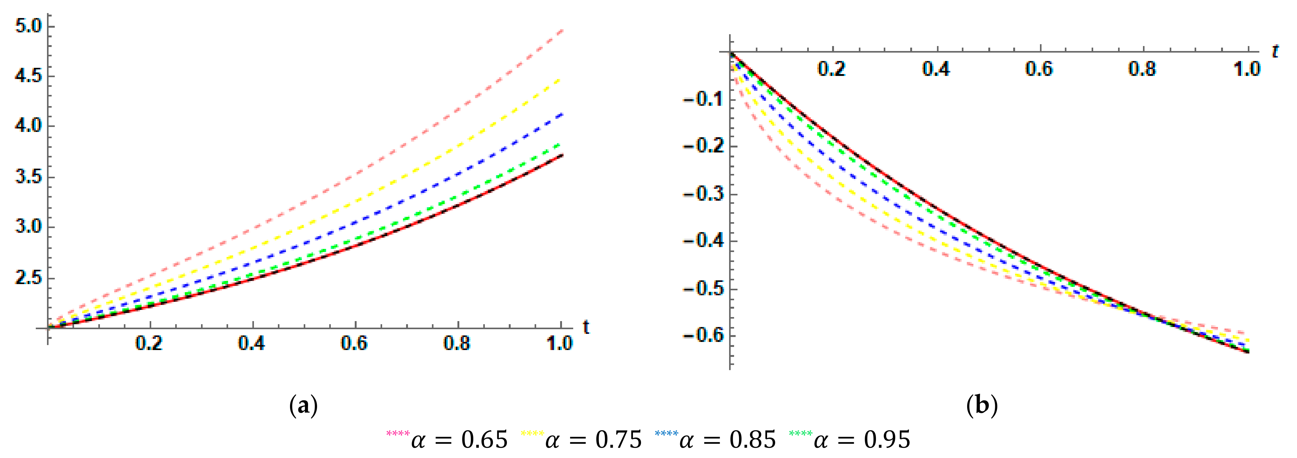
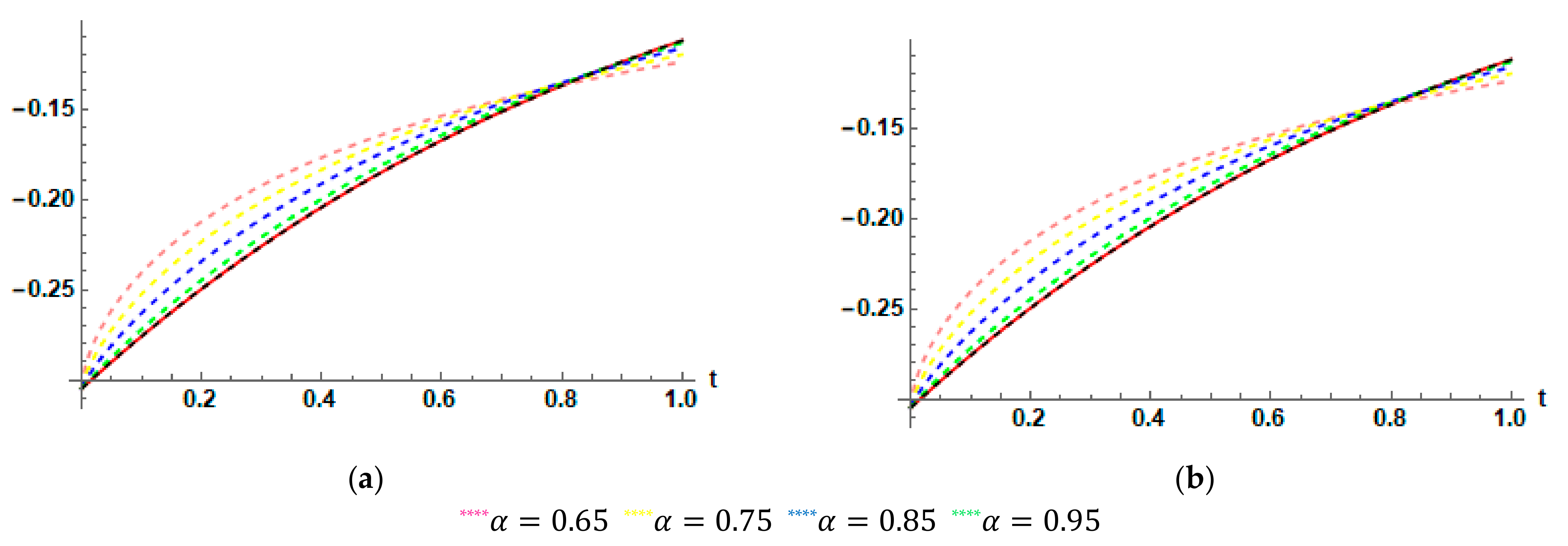
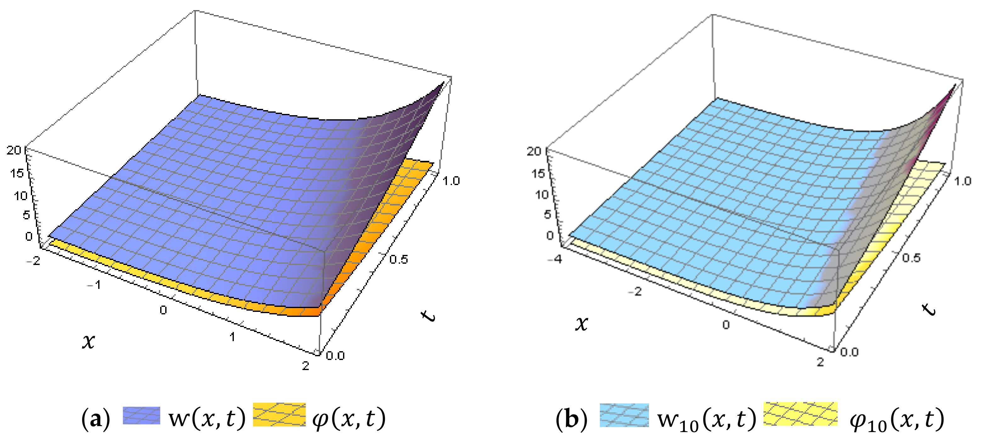
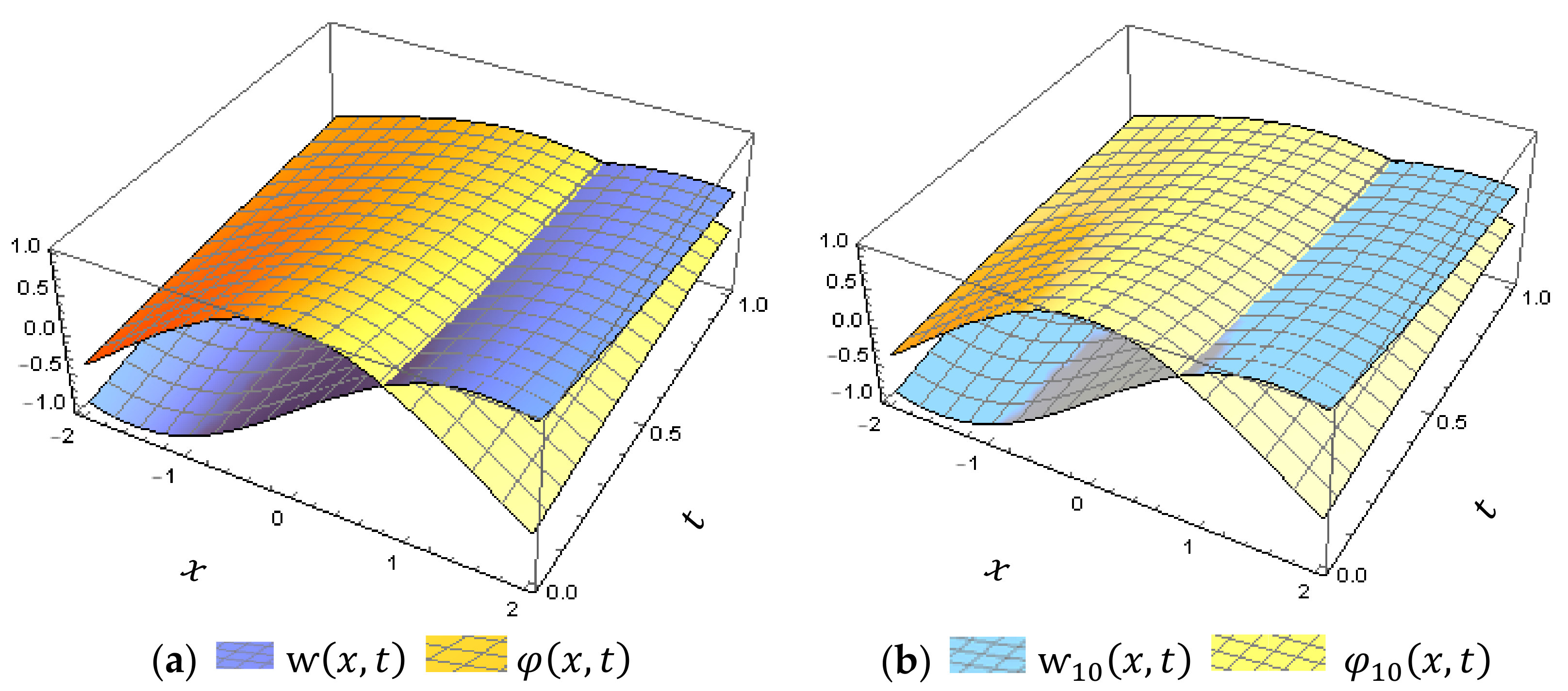
5. Graphical and Numerical Results

This section aims to demonstrate the efficiency, accuracy, and reliability of our proposed method. For this purpose, some of the numerical and graphical results are presented in this section. The efficiency and accuracy of the fractional RPS scheme are validated by obtaining the absolute errors $E_{10}\left(\mathsf{ⱳ}\right)=\left|\mathsf{ⱳ}\left(x,t\right)-{\mathsf{ⱳ}}_{10}\left(x,t\right)\right|$, and $E_{10}\left(\phi \right)=\left|\phi \left(x,t\right)-{\phi }_{10}\left(x,t\right)\right|$, when $\alpha =1$, and at some chosen grid points of $t:0\le t\le 1$ and fixed values of $x$, as shown in

Table 1. Numerical results for Example 1 at $\alpha =1$ and $n=10$ .

$t_i$	Numerical Results of $\mathsf{ⱳ}\left(x,t\right)$
	Exact Solution	Tenth MFPS Solution	$E_{10}\left(\mathsf{ⱳ}\right)$
$0.15$	$2.1618342427282830$	$2.161834242728283$	$0.0$
$0.30$	$2.3498588075760030$	$2.349858807575957$	$4.574118861455645\times {10}^{-14}$
$0.45$	$2.5683121854901687$	$2.568312185486181$	$3.987921104453562\times {10}^{-12}$
$0.60$	$2.8221188003905090$	$2.822118800294857$	$9.565193082039514\times {10}^{-11}$
$0.75$	$3.1170000166126750$	$3.117000015484435$	$1.1282392797795630\times {10}^{-9}$
$0.90$	$3.4596031111569494$	$3.459603102662100$	$8.4948492684588930\times {10}^{-9}$
$t_i$	Numerical Results of $\phi \left(x,t\right)$
	Exact Solution	Tenth MFPS Solution	$E_{10}\left(\phi \right)$
$0.15$	$1.8607079764250578$	$1.8607079764250578$	$1.110223024625156\times {10}^{-16}$
$0.30$	$1.7408182206817178$	$1.7408182206817613$	$4.32986979603811\times {10}^{-14}$
$0.45$	$1.6376281516217732$	$1.6376281516254730$	$3.699485162655946\times {10}^{-12}$
$0.60$	$1.5488116360940265$	$1.5488116361805715$	$8.654510441630237\times {10}^{-11}$
$0.75$	$1.4723665527410148$	$1.4723665537365846$	$9.955698487829068\times {10}^{-10}$
$0.90$	$1.4065696597405992$	$1.4065696670509398$	$7.310340555122252\times {10}^{-9}$

and

Table 2. Numerical results for Example 2 at $\alpha =1,$ and $n=10$.

$t_i$	Numerical Results of $\mathsf{ⱳ}\left(x,t\right)$
	Exact Solution	Tenth MFPS Solution	$E_{10}\left(\mathsf{ⱳ}\right)$
$0.16$	$-0.8419450117729307$	$-0.84194501177293070$	$0.0$
$0.32$	$-0.71745821243338660$	$-0.71745821243347340$	$8.68194405256872\times {10}^{-14}$
$0.48$	$-0.61137755956791100$	$-0.61137755957532720$	$7.416289804496046\times {10}^{-12}$
$0.64$	$-0.52098159009911530$	$-0.52098159027247250$	$1.733572174700270\times {10}^{-10}$
$0.8$	$-0.44395122616870164$	$-0.44395122816140875$	$1.992707110431979\times {10}^{-9}$
$0.96$	$-0.37831027998359285$	$-0.37831029460495413$	$1.462136128838054\times {10}^{-8}$
$t_i$	Numerical Results of $\phi \left(x,t\right)$
	Exact Solution	Tenth MFPS Solution	$E_{10}\left(\phi \right)$
$0.16$	$0.13144441496073755$	$0.13144441496073755$	$0.0$
$0.32$	$0.11200954180308985$	$0.11200954180310340$	$1.35447209004269\times {10}^{-14}$
$0.48$	$0.09544823535245422$	$0.09544823535361205$	$1.15782383680596\times {10}^{-12}$
$0.64$	$0.08133562092337902$	$0.08133562095044355$	$2.70645311717388\times {10}^{-11}$
$0.8$	$0.06930964419156765$	$0.0693096445026690$	$3.11101339134368\times {10}^{-10}$
$0.96$	$0.05906178281330243$	$0.05906178509598864$	$2.282686213661566\times {10}^{-9}$

. Moreover, some numerical solutions are computed for the tenth MFPS approximate solutions as discussed in Examples 1 and 2 for various values of parameter $\alpha$ and are summarized in

Table 3. Numerical results of approximated solutions, at $n=10$, with different values of $\alpha$, for Example 1.

$t_i$	${\mathsf{ⱳ}}_{10}\left(x,t\right)$
	$\alpha =1$	$\alpha =0.90$	$\alpha =0.80$	$\alpha =0.60$
$0.2$	$2.2214027581601690$	$2.2805331573375804$	$2.3574062080626383$	$2.5992370899310580$
$0.4$	$2.4918246976401830$	$2.5937448915963692$	$2.7226080973587683$	$3.1141975607216192$
$0.6$	$2.8221188002948576$	$2.9688456557530300$	$3.1525814312710714$	$3.7044906449490766$
$0.8$	$3.2255409261876826$	$3.4229421259078268$	$3.6691633475212875$	$4.4052769051540555$
$1.00$	$3.7182818011463845$	$3.9749386808012870$	$4.2945640956260980$	$5.2480111300443130$
$t_i$	${\phi }_{10}\left(x,t\right)$
	$\alpha =1$	$\alpha =0.90$	$\alpha =0.80$	$\alpha =0.60$
$0.2$	$-0.18126924692201762$	$-0.2142375812825914$	$-0.2493747318757895$	$-0.32154982625236140$
$0.4$	$-0.32967995396334393$	$-0.3589009729302870$	$-0.3856516643965252$	$-0.42947454232435334$
$0.6$	$-0.45118836381942860$	$-0.4688859797736396$	$-0.4824316301790333$	$-0.49835879852667764$
$0.8$	$-0.55067103386593300$	$-0.5551187066686112$	$-0.5556567450518857$	$-0.5481336616645864$
$1.00$	$-0.63212053571428560$	$-0.6239336668417425$	$-0.6130477144305024$	$-0.5863356183976949$

and

Table 4. Numerical results of approximate solutions, at $n=10$, with different values of $\alpha$, for Example 2.

$t_i$	${\mathsf{ⱳ}}_{10}\left(x,t\right)$
	$\alpha =1$	$\alpha =0.90$	$\alpha =0.80$	$\alpha =0.60$
$0.25$	$-0.7694798025428385$	$-0.73647409969579200$	$-0.7027615522135062$	$-0.6377598728012623$
$0.50$	$-0.5992714727895893$	$-0.57564053036593310$	$-0.5555897076872737$	$-0.5265590627538489$
$0.75$	$-0.4667130932555057$	$-0.45904510752654604$	$-0.4554206561883250$	$-0.4574845903163597$
$1.00$	$-0.3634765445686263$	$-0.37156542991700050$	$-0.3823210951576755$	$-0.4087134907838949$
$t_i$	${\phi }_{10}\left(x,t\right)$
	$\alpha =1$	$\alpha =0.90$	$\alpha =0.80$	$\alpha =0.60$
$0.25$	$0.12013114996235093$	$0.11497830121280808$	$0.10971509991262596$	$0.09956704083235894$
$0.50$	$0.09355823366375775$	$0.08986897206304160$	$0.08673863858564738$	$0.08220637568741900$
$0.75$	$0.07286322579226955$	$0.07166610022708808$	$0.07110025105755274$	$0.07142247235488633$
$1.00$	$0.05674594074993913$	$0.05800877714356845$	$0.05968795108640946$	$0.06380833062900641$

. From these tables, one can see that our present approach provides accurate approximate solutions which are in a good agreement with the exact solutions, although only ten terms of MFPS approximate solutions are utilized to achieve this accuracy. The accuracy can be increased by adding extra terms which makes the overall error smaller. Moreover,

Table 5. Numerical comparisons between the absolute errors for Example 1.

$\mathit{t}$	${\mathit{x}}_{\mathit{i}}$	LRPSM		LADM
		$\left| \mathit{ⱳ}\left(\mathit{x},\mathit{t}\right)-{\mathit{ⱳ}}_{10}\left(\mathit{x},\mathit{t}\right)\right|$	$\left| \mathit{\phi }\left(\mathit{x},\mathit{t}\right)-{\mathit{\phi }}_{10}\left(\mathit{x},\mathit{t}\right)\right|$	$\left| \mathit{ⱳ}\left(\mathit{x},\mathit{t}\right)-{\mathit{ⱳ}}_{10}\left(\mathit{x},\mathit{t}\right)\right|$	$\left| \mathit{\phi }\left(\mathit{x},\mathit{t}\right)-{\mathit{\phi }}_{10}\left(\mathit{x},\mathit{t}\right)\right|$
	$-4$	$0.0$	$0.0$	$3.6792791036\times {10}^{-12}$	$3.5893510386\times {10}^{-13}$
$0.1$	$-3$	$0.0$	$0.0$	$1.0003109452\times {10}^{-13}$	$9.7566399405\times {10}^{-13}$
	$-2$	$0.0$	$1.1102230246\times {10}^{-16}$	$2.7191582319\times {10}^{-12}$	$2.6521007612\times {10}^{-12}$
	$-1$	$2.2204460493\times {10}^{-16}$	$1.1102230246\times {10}^{-16}$	$7.3914208087\times {10}^{-12}$	$7.2091221881\times {10}^{-12}$
	$0$	$0.0$	$1.1102230246\times {10}^{-16}$	$2.0091928121\times {10}^{-12}$	$1.9596102518\times {10}^{-11}$
	$1$	$1.7763568394\times {10}^{-15}$	$0.0$	$5.4615867384\times {10}^{-11}$	$5.3267168454\times {10}^{-11}$
	$2$	$0.0$	$1.77635683940\times {10}^{-15}$	$1.4846079921\times {10}^{-11}$	$1.4479706322\times {10}^{-10}$
$1$	$-4$	$5.0024873133\times {10}^{-10}$	$4.2335268624\times {10}^{-10}$	$4.1443327905\times {10}^{-10}$	$3.2256474624\times {10}^{-6}$
	$-3$	$1.3598173698\times {10}^{-9}$	$1.1507917952\times {10}^{-9}$	$1.1265464516\times {10}^{-6}$	$8.7682188824\times {10}^{-6}$
	$-2$	$3.6963667682\times {10}^{-9}$	$3.1281764956\times {10}^{-9}$	$3.0622707483\times {10}^{-5}$	$2.3834490061\times {10}^{-5}$
	$-1$	$1.0047766175\times {10}^{-8}$	$8.5032654252\times {10}^{-9}$	$8.3241149288\times {10}^{-5}$	$6.4788861210\times {10}^{-5}$
	$0$	$2.7312660578\times {10}^{-8}$	$2.3114271941\times {10}^{-8}$	$2.2627290349\times {10}^{-4}$	$1.7611438411\times {10}^{-4}$
	$1$	$7.4243510895\times {10}^{-8}$	$6.2831105429\times {10}^{-8}$	$6.1507352183\times {10}^{-4}$	$4.7872853007\times {10}^{-4}$
	$2$	$2.0181478178\times {10}^{-7}$	$1.7079265247\times {10}^{-7}$	$1.6719431776\times {10}^{-3}$	$1.3013190640\times {10}^{-3}$

presents the absolute errors of the tenth FPS approximate solutions of the linear system of FPDEs (7) and (8) which are computed by LRPSM and compared with the computed absolute errors by the Laplace–Adomian decomposition method (LADM) [31] at the standard-case $\alpha =1$. The simulation of Table 5 confirms that the proposed method is more accurate and faster than LADM to determine the exact solutions of system (7) and (8). Graphically, the tenth MFPS approximate solutions versus the exact solutions for the above-solved systems of FPDEs are plotted in three-dimensional space for $t\in \left[0,1\right]$, and $x\in \left[-2,2\right]$, when $\alpha =1$, as shown in Figure 1 and Figure 2. It is clear that the pattern of the exact solutions is consistent and in good agreement with the pattern of the approximate solutions in their domains, and this confirms the effectiveness and performance of fractional RPS scheme. However, Figure 3 and Figure 4 show the impact of the parameter on curves of the MFPS approximate solutions for $\alpha \in \left\{0.65,0.75,0.85,0.95,1\right\}$, $t\in \left[0,1\right]$, and fixed values of $x$ against the exact solutions. Here, one can notice that the curves of the solutions are compatible with each other and in a homogeneous fashion. When the parameter α is increasing in its domain, the curves of the solutions converge to the standard sense $\alpha =1$.

6. Conclusions

In this work, the exact and approximate solutions for certain systems of FPDEs were created successfully using a recent attractive method based on the fractional RPS. The proposed technique is used to determine expansion coefficients in an easy systematic manner that depends basically on the Caputo fractional derivative for each phase. The efficiency and applicability of our technique in producing the solutions for the systems of FPDEs have been tested via two illustrative examples. The analysis of the obtained results of fractional RPS were shown to be fully compatible between the exact and approximate solutions, and also with the results obtained by other methods. The accuracy of the proposed technique is tested by comparing the numerical simulations of the FRPS-absolute errors with those computed using LADM [31]. It was shown that the FRPS technique provides high accuracy and yields accurate approximations more than LADM. This confirms that our proposed algorithm is a promising method. Consequently, the application of the fractional RPS method can be extended to handle a wide class of fractional physical models. In future study, the application of the current algorithm can be extended to deal with different types of dynamical evolution models, stochastic models, inverse uncertain systems, and quantum physics imposed by nonclassical conditions.

References

1. Mainardi, F.; Raberto, M.; Gorenflo, R.; Scalas, E. Fractional calculus and continuous-time finance II: The waiting-time distribution. Phys. A: Stat. Mech. Its Appl. 2000, 287, 468–481. [Google Scholar] [CrossRef] [Green Version]
2. Alabedalhadi, M.; Al-Smadi, M.; Al-Omari, S.; Baleanu, D.; Momani, S. Structure of optical soliton solution for nonliear resonant space-time Schrödinger equation in conformable sense with full nonlinearity term. Phys. Scr. 2020, 95, 105215. [Google Scholar] [CrossRef]
3. Caputo, M. Linear models of dissipation whose Q is almost frequency independent—II. Geophys. J. Int. 1967, 13, 529–539. [Google Scholar] [CrossRef]
4. Al-Smadi, M.; Arqub, O.A. Computational algorithm for solving fredholm time-fractional partial integrodifferential equations of Dirichlet functions type with error estimates. Appl. Math. Comput. 2019, 342, 280–294. [Google Scholar] [CrossRef]
5. Xu, H.; Liao, S.-J.; You, X.-C. Analysis of nonlinear fractional partial differential equations with the homotopy analysis method. Commun. Nonlinear Sci. Numer. Simul. 2009, 14, 1152–1156. [Google Scholar] [CrossRef]
6. Jleli, M.; Kumar, S.; Kumar, R.; Samet, B. Analytical approach for time fractional wave equations in the sense of Yang-Abdel-Aty-Cattani via the homotopy perturbation transform method. Alex. Eng. J. 2020, 59, 2859–2863. [Google Scholar] [CrossRef]
7. Hasan, S.; Al-Smadi, M.; El-Ajou, A.; Momani, S.; Hadid, S.; Al-Zhour, Z. Numerical approach in the Hilbert space to solve a fuzzy Atangana-Baleanu fractional hybrid system. Chaos Solitons Fractals 2021, 143, 110506. [Google Scholar] [CrossRef]
8. Hasan, S.; El-Ajou, A.; Hadid, S.; Al-Smadi, M.; Momani, S. Atangana-Baleanu fractional framework of reproducing kernel technique in solving fractional population dynamics system. Chaos Solitons Fractals 2020, 133, 109624. [Google Scholar] [CrossRef]
9. Al-Smadi, M.; Abu Arqub, O.; Gaith, M. Numerical simulation of telegraph and Cattaneo fractional-type models using adaptive reproducing kernel framework. Math. Methods Appl. Sci. 2021, 44, 8472–8489. [Google Scholar] [CrossRef]
10. Al-Smadi, M.; Freihat, A.; Khalil, H.; Momani, S.; Ali Khan, R. Numerical multistep approach for solving fractional partial differential equations. Int. J. Comput. Methods 2017, 14, 1750029. [Google Scholar] [CrossRef]
11. Momani, S.; Arqub, O.A.; Freihat, A.; Al-Smadi, M. Analytical approximations for Fokker-Planck equations of fractional order in multistep schemes. Appl. Comput. Math. 2016, 15, 319–330. [Google Scholar]
12. Das, S. Analytical solution of a fractional diffusion equation by variational iteration method. Comput. Math. Appl. 2009, 57, 483–487. [Google Scholar] [CrossRef] [Green Version]
13. Kumar, S. A new fractional modeling arising in engineering sciences and its analytical approximate solution. Alex. Eng. J. 2013, 52, 813–819. [Google Scholar] [CrossRef] [Green Version]
14. Al-Smadi, M. Simplified iterative reproducing kernel method for handling time-fractional BVPs with error estimation. Ain Shams Eng. J. 2018, 9, 2517–2525. [Google Scholar] [CrossRef]
15. Saadeh, R.; Alaroud, M.; Al-Smadi, M.; Ahmad, R.R.; Din, U.K.S. Application of fractional residual power series algorithm to solve Newell–Whitehead–Segel equation of fractional order. Symmetry 2019, 11, 1431. [Google Scholar] [CrossRef] [Green Version]
16. Freihet, A.; Hasan, S.; Al-Smadi, M.; Gaith, M.; Momani, S. Construction of fractional power series solutions to fractional stiff system using residual functions algorithm. Adv. Differ. Equ. 2019, 2019, 95. [Google Scholar] [CrossRef] [Green Version]
17. Al-Smadi, M. Fractional residual series for conformable time-fractional Sawada–Kotera–Ito, Lax, and Kaup–Kupershmidt equations of seventh order. Math. Methods Appl. Sci. 2021. Early View. [Google Scholar] [CrossRef]
18. Freihet, A.; Hasan, S.; Alaroud, M.; Al-Smadi, M.; Ahmad, R.R.; Din, U.K.S. Toward computational algorithm for time-fractional Fokker–Planck models. Adv. Mech. Eng. 2019, 11, 1–11. [Google Scholar] [CrossRef]
19. Al-Smadi, M.; Arqub, O.A.; Hadid, S. Approximate solutions of nonlinear fractional Kundu-Eckhaus and coupled fractional massive Thirring equations emerging in quantum field theory using conformable residual power series method. Phys. Scr. 2020, 95, 105205. [Google Scholar] [CrossRef]
20. Al-Smadi, M.; Arqub, O.A.; Momani, S. Numerical computations of coupled fractional resonant Schrödinger equations arising in quantum mechanics under conformable fractional derivative sense. Phys. Scr. 2020, 95, 075218. [Google Scholar] [CrossRef]
21. Kumar, A.; Kumar, S.; Singh, M. Residual power series method for fractional Sharma-Tasso-Olever equation. Commun. Numer. Anal. 2016, 2016, 1–10. [Google Scholar] [CrossRef]
22. Al-Smadi, M.; Arqub, O.A.; Hadid, S. An attractive analytical technique for coupled system of fractional partial differential equations in shallow water waves with conformable derivative. Commun. Theor. Phys. 2020, 72, 085001. [Google Scholar] [CrossRef]
23. Alaroud, M.; Al-Smadi, M.; Ahmad, R.R.; Din, U.K.S. An analytical numerical method for solving fuzzy fractional Volterra integro-differential equations. Symmetry 2019, 11, 205. [Google Scholar] [CrossRef] [Green Version]
24. Alaroud, M.; Al-Smadi, M.; Ahmad, R.R.; Din, U.K.S. Computational optimization of residual power series algorithm for certain classes of fuzzy fractional differential equations. Int. J. Differ. Equ. 2018, 2018, 8686502. [Google Scholar] [CrossRef]
25. Alaroud, M.; Ahmad, R.R.; Din, U.K.S. An efficient analytical-numerical technique for handling model of fuzzy differential equations of fractional-order. Filomat 2019, 33, 617–632. [Google Scholar] [CrossRef] [Green Version]
26. Abuteen, E.; Freihat, A.; Al-Smadi, M.; Khalil, H. Approximate series solution of nonlinear, fractional Klein-Gordon equations using fractional reduced differential transform method. J. Math. Stat. 2016, 12, 23–33. [Google Scholar] [CrossRef] [Green Version]
27. Al-Smadi, M.; Arqub, O.A.; Zeidan, D. Fuzzy fractional differential equations under the Mittag-Leffler kernel differential operator of the ABC approach: Theorems and applications. Chaos Solitons Fractals 2021, 146, 110891. [Google Scholar] [CrossRef]
28. Al-Smadi, M.; Djeddi, N.; Momani, S.; Al-Omari, S.; Araci, S. An attractive numerical algorithm for solving nonlinear Caputo–Fabrizio fractional Abel differential equation in a Hilbert space. Adv. Differ. Equ. 2021, 2021, 271. [Google Scholar] [CrossRef]
29. Al-Smadi, M.; Dutta, H.; Hasan, S.; Momani, S. On numerical approximation of Atangana-Baleanu-Caputo fractional integro-differential equations under uncertainty in Hilbert Space. Math. Model. Nat. Phenom. 2021, 16, 41. [Google Scholar] [CrossRef]
30. Korpinar, Z.; Inc, M.; Hınçal, E.; Baleanu, D. Residual power series algorithm for fractional cancer tumor models. Alex. Eng. J. 2020, 59, 1405–1412. [Google Scholar] [CrossRef]
31. Ahmed, H.F.; Bahgat, M.S.; Zaki, M. Numerical approaches to system of fractional partial differential equations. J. Egypt. Math. Soc. 2017, 25, 141–150. [Google Scholar] [CrossRef]
32. Dhaigude, D.; Kanade, S.N.; Dhaigude, C. Solution for System of Fractional Partial Differential Equations. Appl. Appl. Math. 2018, 13, 259–273. [Google Scholar]
Figure 1. (a) 3D-surfaces plot of exact solutions x , t and φ x , t at α = 1 ; (b) 3D-surfaces plot of tenth MFPS approximate solutions 10 x , t and φ 10 x , t at α = 1 , for Example 1.
Mathematics 09 02868 g001
Figure 2. (a) 3D-surfaces plot of exact solutions x , t and φ x , t at α = 1 ; (b) 3D-surfaces plot of tenth MFPS approximate solutions 10 x , t and φ 10 x , t at α = 1 , for Example 2.
Mathematics 09 02868 g002
Figure 3. (a) Plot of exact solutions x , t and 10 x , t at various values of α ; (b) plot of exact solutions φ x , t and φ 10 x , t at various values of α , for Example 1.
Mathematics 09 02868 g003
Figure 4. (a) Plot of exact solutions x , t and 10 x , t at various values of α ; (b) plot of exact solutions φ x , t and φ 10 x , t at various values of α , for Example 2.
Mathematics 09 02868 g004