1. Introduction
Diagnostic tests are fundamental in the current practice of medicine. A diagnostic test is a medical test that is applied to an individual to determine the presence or absence of a disease [
1]. Diagnostic tests can be binary, ordinal or continuous. Binary tests give two possible results: positive or negative. An antigen test for the diagnosis of COVID-19 is an example of a binary diagnostic test. Ordinal tests classify the presence of the disease in different ordinal categories. For example, in the diagnosis of breast cancer, malignant lesions can be classified as “malignant, suspicious, probably benign, benign or normal”. With respect to continuous tests, these give rise to continuous values, for example procalcitonin for the diagnosis of infective endocarditis. The efficacy of a diagnostic test is evaluated against a gold standard. A gold standard (GS) is a medical test that objectively determines whether or not an individual has the disease. For example, a biopsy for the diagnosis of cancer. This article focuses on binary diagnostic tests.
The fundamental measures to evaluate the effectiveness of a binary diagnostic test (BDT) are sensitivity and specificity. Sensitivity is the probability that the test result is positive when the individual has the disease, and specificity is the probability that the test result is negative when the individual does not have the disease. The sensitivity and specificity of a BDT depend on the physical, chemical or biological bases with which the test has been developed. When evaluating the effectiveness of a BDT considering the losses associated with misclassification with the BDT, the parameter used is the weighted kappa coefficient [
1,
2]. The weighted kappa coefficient is a parameter that measures the beyond chance agreement between BDT and GS [
1,
2], and depends on the sensitivity and specificity of BDT, on the disease prevalence and on the weighting index. The weighting index is a measure of the relative importance between false positives and false negatives. In practice, the weighting index
c is set by the clinician depending on the clinical use of the BDT (for example, confirmatory test or screening test) and the clinician’s knowledge of the importance of a false positive and a false negative. If the BDT is to be used as a confirmatory test, then the weighting index takes a value between 0 and 0.5. If the BDT is to be used as a screening test, then the weighting index takes a value between 0.5 and 1. The problem with the weighted kappa coefficient is the assignment of values to the weighting index
c, since the clinician does not always have a knowledge that allows him to decide how important a false positive is compared to a false negative. Even in the same problem, two clinicians can assign different values to the weighting index. Roldán-Nofuentes and Olvera-Porcel [
3] have defined and studied a new measure to evaluate the effectiveness of a BDT: the average kappa coefficient. The average kappa coefficient depends only on the intrinsic accuracy (sensitivity and specificity) of the BDT and on the disease prevalence, and is a parameter that does not depend on the weighting index. Therefore, the average kappa coefficient is a parameter that solves the problem of assigning values to the weighting index. Average kappa coefficient is a measure of the average beyond-chance agreement between the BDT and the GS [
3].
Comparison of the effectiveness of two BDTs is a topic of special interest in the study of statistical methods for the diagnosis of diseases. The most frequent type of sampling to compare two BDTs is the paired design, which consists of applying the two BDTs to all individuals in a random sample whose disease status is known by applying a GS. Bloch [
4] has studied the comparison of the weighted kappa coefficients of two BDTs under a paired design, and Roldán-Nofuentes and Luna [
5] have extended the study of Bloch to the situation in which the weighted kappa coefficients of more than two BDTs are compared. Roldán-Nofuentes and Olvera-Porcel [
6] has studied the comparison of the average kappa coefficients of two BDTs under a paired design. However, in clinical practice the GS is not always applied to all individuals in the sample. Consequently, the disease state is unknown for a subset of individuals in the sample. This problem is known as partial verification of disease [
7,
8]. Zhou [
9] has studied a hypothesis test to compare the sensitivities (specificities) of two BDTs in the presence of partial verification, applying the maximum likelihood method. If in this situation the two sensitivities (specificities) are compared, eliminating the individuals whose disease status is unknown, the estimates obtained are biased (the estimators are affected by the so-called verification bias [
7]) and the results may be incorrect [
9]. Harel and Zhou [
10] have compared the sensitivities (specificities) of two BDTs using confidence intervals applying multiple imputation, and Roldán-Nofuentes and Luna [
11] have compared the sensitivities (specificities) by applying the EM and the SEM algorithms. Roldán-Nofuentes and Luna [
12] have studied a hypothesis test to compare the weighted kappa coefficients of two BDTs in the presence of partial verification of the disease, applying the maximum likelihood method. Regarding the average kappa coefficient, Roldán-Nofuentes and Regad [
13] have studied the estimation of this parameter when only a single BDT is evaluated in the presence of partial verification, applying the maximum likelihood method and multiple imputation. The comparison of the average kappa coefficients of two BDTs has never been studied in the presence of partial verification. In this situation, if the weighted kappa coefficients are compared, eliminating the unverified individuals with the GS, then the estimators of the weighted kappa coefficients are biased [
12], and therefore the estimators of the average kappa coefficients, and the conclusions can also be incorrect. Consequently, the method of Roldán-Nofuentes and Olvera-Porcel [
6] cannot be applied in the presence of partial verification.
In this article, the comparison of the average kappa coefficients of two BDTs in the presence of partial verification of the disease is studied. Therefore, the objective of our manuscript is to study a hypothesis test to compare the average kappa coefficients of two BDTs in the presence of partial verification, a topic that has never been studied. This article is an extension of the article by Roldán-Nofuentes and Olvera-Porcel [
6] to the situation in which the GS does not apply to all the individuals in the sample, and is also an extension of the article by Roldán-Nofuentes and Regad [
13] to the situation where two BDTs are compared in the presence of partial verification. The article is structured as follows. In
Section 2 the average kappa coefficient and its properties are presented. In
Section 3 we study the comparison of the weighted kappa coefficients of two BDTs in the presence of partial verification of the disease, applying two computational methods: the EM algorithm and the SEM algorithm. In
Section 4, a function written in R is presented to solve the problem and simulation experiments are carried out to study the size and power of the method to solve the hypothesis test for the comparison of the two average kappa coefficients. In
Section 5 the results are applied to the diagnosis of Alzheimer disease, and in
Section 6 the results obtained are discussed.
2. Average Kappa Coefficient
Let us consider two BDTs, Test 1 and Test 2, whose performances are compared with respect to the same GS. Let
(
) be the loss that occurs when a BDT gives a negative (positive) result for a diseased (non-diseased) patient. Loss
is associated with a false negative and loss
is associated with a false positive [
1,
2]. Losses are assumed to be zero when a BDT correctly classifies a diseased patient or a non-diseased patient [
1,
2]. For example, let us consider the diagnosis of renal cell carcinoma using the MOC 31. If the MOC 31 is positive for an individual without the renal carcinoma (false positive), the individual will undergo a renal biopsy which will be negative. Loss
is determined by the economic costs of the diagnosis and also by the risk, stress, etc, caused to the individual. If the MOC 31 is negative for an individual with renal carcinoma (false negative), the individual will be diagnosed later, but the cancer will progress and get worse, decreasing the chance that treatment will be successful. Loss
is determined from this situation. Therefore, losses
and
are measured in terms of economic costs and in terms of risks, stress, etc [
1,
2], so in clinical practice it is not possible to know
and
. Let
T be the binary random variable that models the result of the BDT, in such a way that
when the result is positive and
when the result is negative. Let
D be the binary random variable that models the result of the GS, in such a way that
when the individual has the disease and
when the individual does not have the disease. In
Table 1, we show the losses and probabilities associated with the assessment of a BDT in relation to a GS, where
Se is the sensitivity,
Sp the specificity and
p the disease prevalence.
In terms of the losses and probabilities in
Table 1, the expected loss [
4] is
and the random loss [
4] is
, with
. The expected loss is the loss that occurs when erroneously classifying a diseased or non-diseased individual with the BDT. The expected loss varies between zero and infinity. The random loss is the loss that occurs when the BDT and the GS are independent, i.e., when
. In terms of these losses, the weighted kappa coefficient is defined as [
1,
2,
4]
since
. Performing algebraic operations, the weighted kappa coefficient is written as [
1,
2,
4]
where
is the Youden index [
14] of the
hth Test,
is the probability that the
hth Test is positive and
is the weighting index. The weighted kappa coefficient of the
hth Test can also be written as
where
As
and
are unknown, the clinician sets the value of the weighting index based on the relative importance between false positives and false negatives [
1,
2]. If the clinician considers that false positives are more important than false negatives, as is the situation in which the BDT is used as a confirmatory test prior to the application of a risk treatment (for example a surgical operation), then
and
. For example, if a false positive is four times more important than a false negative then
and
. If the clinician considers that false negatives are more important than false positives, as is the situation in which the BDT is used as a screening test, then
and
. For example, if a false negative is three times more important than a false positive then
and
. Value
is used when false positives and false negatives have the same importance, being
the Cohen kappa coefficient. The weighted kappa coefficient has the following properties [
1,
2,
4]:
- 1.
If then , and the agreement between Test and GS is perfect.
- 2.
If then , and the Test and the GS are independent.
- 3.
Weighted kappa coefficient is a function of the index c, which is increasing if , decreasing if , or equal to the Youden index if .
The weighted kappa coefficient can be classified in the following scale of values [
15]:
, slight;
, fair;
, moderate;
, substantial; and
, almost perfect. Another scale based on levels of clinical significance is [
16]:
, poor;
, fair;
, good; and
, excellent.
Roldán-Nofuentes and Olvera-Porcel [
3] have proposed a new measure to evaluate and to compare BDTs: the average kappa coefficient. If
, and therefore
, the average kappa coefficient of the
hth Test is [
3]
i.e., the average kappa coefficient is the average value of
when
. If
and therefore
, the average kappa coefficient of the
hth Test is [
3]
i.e., the average kappa coefficient is the average value of
when
. As the weighted kappa coefficient is a measure of the beyond-chance agreement between a BDT and the GS, the average kappa coefficient is a measure of the average beyond-chance agreement between a BDT and a GS [
3], and does not depend on the weighting index
. As
and
depend on
,
and
, then
and
also depend on these same parameters. The values of the average kappa coefficient can be classified on the same scales [
15,
16] as the values of the weighted kappa coefficient [
3]. The average kappa coefficients
and
have the following properties [
3]:
- 1.
If then , and if then . Therefore , .
- 2.
if and if .
- 3.
minimizes and minimizes . Therefore, when () the first (second) expression is the variance of around ().
- 4.
For fixed values of and , the weighted kappa coefficient is a function of which is continuous in the interval . Therefore, the average kappa coefficient is equal to a value of in the interval . This value of has a value of weighting index . So, as for some value of , from Equation (1) and for a specific sample it is possible to calculate the value of c associated to the estimated of . Therefore, the estimation of allows estimating how much greater (or less) the loss is than the loss .
Next, the comparison of the average kappa coefficients of two BDTs in the presence of partial verification of the disease is studied.
3. Comparison of Average Kappa Coefficients
The objective of this manuscript is to study the hypothesis tests
and
when not all patients in a random sample are verified with the GS. The first hypothesis test is used when the clinician considers that
(
) and the second hypothesis test is used when the clinician considers that
(
). Both hypothesis tests will be solved by applying two computational methods: the EM algorithm and the SEM algorithm. The EM algorithm [
17] is a classic method to estimate parameters with missing data, and the SEM (Supplemented EM) algorithm [
18] is a method that allows estimating the variances-covariances of a vector of parameters from the results obtained by applying the EM algorithm.
In the problem posed here, the sample design is as follows: two BDTs are applied to all individuals of a random sample sized
n and the GS is applied only to a subset of the
n individuals. This situation gives rise to
Table 2, where
is the binary random variable that models the result of the
hth Test (
when the Test is positive and
when it is negative),
V is the binary random variable that models the verification process (
when the disease status of an individual is verified with the GS and
when the disease status of an individual is not verified with the GS), and
D is the binary random variable that models the GS ( when the individual verified with the GS has the disease and
when the individual verified with the GS does not have the disease and
when the individual verified with the GS does not have the disease). In this table, each frequency
(
) is the number of diseased (non-diseased) individuals in which
and
(
), each frequency
is the number of individuals not verified with the GS in which and
and
,
,
,
,
and
.
Let
and
be the sensitivity and the specificity of the
hth Test, let
be the disease prevalence, and let
be the probability of verifying with the GS an individual with results
,
and
, with
and
. Assuming that the verification process is missing at random (MAR) [
19], i.e., that the probability of verifying with the GS the disease status of an individual only conditionally depends on the results of both BDTs, then
. If the disease status of an individual is not verified with the GS, this individual can be considered as a missing value of the disease status, and then missing data analysis methods can be used to compare two BDTs in the presence of partial verification of the disease. The MAR assumption has been widely used in this context to compare parameters of two BDTs [
9,
10,
11,
12]. Assuming the MAR assumption, the frequencies in
Table 1 are the product of a multinomial distribution sized
n, whose probabilities are:
where
,
if
and
if
,
(
) is the covariance [
20] between the two BDTs when
(
), verifying that
and
. If
then the two BDTs are conditionally independent on the disease, a situation which is not realistic in practice so that
and/or
. Solving the system of equations
and
, with
, it is obtained that
and substituting these expressions in Equation (6), the probabilities of the multinomial distribution are obtained in terms of the weighted kappa coefficients. Next we apply the EM algorithm to obtain the estimates of the parameters.
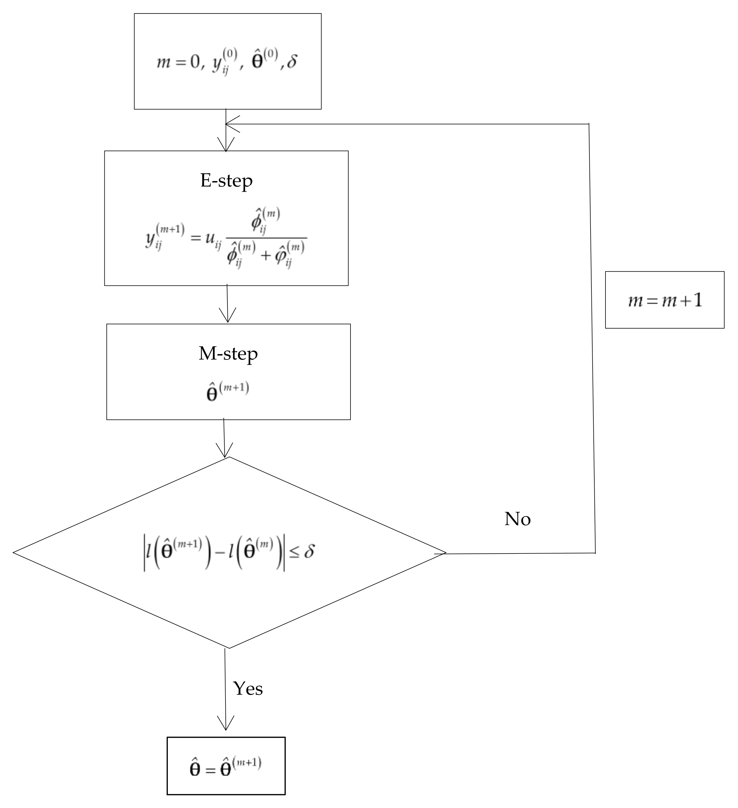
The maximum likelihood (ML) estimates of the parameters are obtained by applying the EM algorithm [
17]. The EM algorithm is a computational method that allows estimating parameters in the presence of missing data, and it is a method widely used in statistics to solve estimation problems in different areas, for example in industrial engineering [
21] and in epidemiology [
22]. Next, we carry out a reparametrization of the EM algorithm that allows us to estimate the weighted kappa coefficients of the two BDTs (and therefore the average kappa coefficients), the covariances and the disease prevalence. In
Table 2 the missing data is the true disease status of the individuals who are not verified with the GS; this information is reconstructed in the E step of the EM algorithm. In the M step the ML estimates are imputed. Let us assume that that among the
individuals not verified with the GS,
have the disease and
do not have the disease. Then the data can be expressed in the form of a
table with frequencies
for
and
, with
. Let
be the vector of parameters. From the complete data, the log-likelihood function based on
n individuals is
where
In these probabilities, covariances
and
verify Equation (7),
and
are given by Equation (8), and it is verified that
. The vector
is estimated by applying the EM algorithm. Let
be the value of
in the
mth iteration of the EM algorithm and
.
ML estimate of
in the
mth iteration,
, is:
The ML estimate of
in the
th iteration,
, is calculated applying the previous equations substituting
with
, where
and where
(
) is the estimate of
(
) in the
mth iteration and it is obtained substituting in
(
) the parameters with their respective estimates obtained in the
mth iteration of the algorithm. As initial value
one can take any value
,
. The EM algorithm stops when the difference between the values of the log-likelihood functions of two consecutive iterations is equal to or less than a value
, for example
. If the EM algorithm converges in M iterations,
is the final estimate obtained. The estimates of the weighted kappa coefficients obtained by applying the EM algorithm converge to the ML estimates (proof can be seen in
Appendix A).
Figure 1 shows the flowchart of the EM algorithm to estimate
.
Once the value of
and
have been imputed, the estimates of average kappa coefficients are easily calculated by applying Equations (2) and (3), i.e.,
and
The estimates of
and
are calculated as:
where
. Once the ML estimates have been obtained, it is necessary to estimate their variances-covariances. For this we apply the Supplemented EM algorithm.
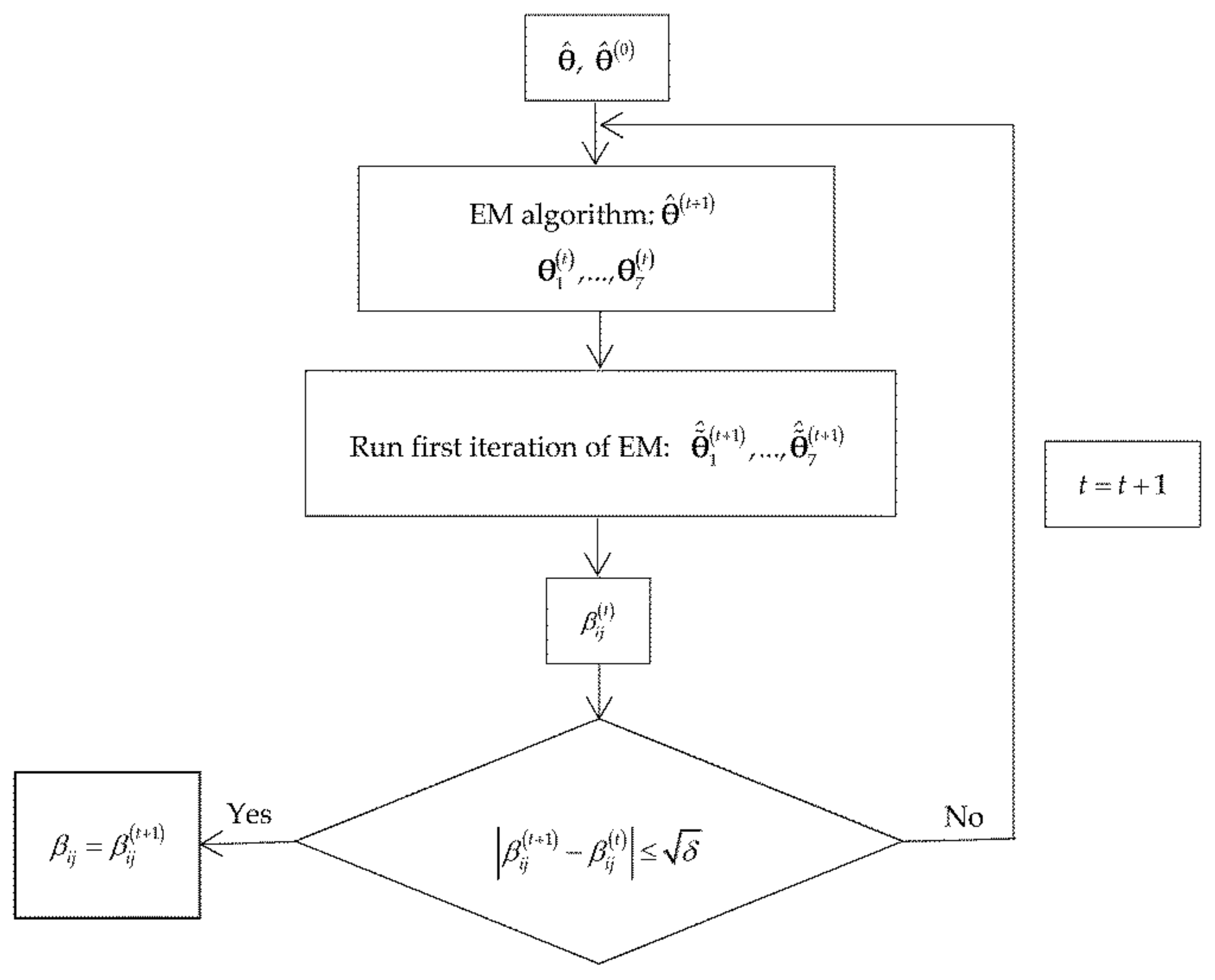
The variance-covariance matrix of
is estimated by applying the supplemented EM (SEM) algorithm [
18]. The SEM algorithm is a computational method which estimates the variances-covariances matrix from the calculations obtained by applying the EM algorithm. Dempster et al. [
17] have shown that the matrix of variance-covariance of
is expressed as
where
is the identity matrix,
,
is the Fisher information matrix of complete data and
is the Fisher information matrix of missing data. The application of the SEM algorithm consists of three steps [
18]: (1) calculate the matrix
, (2) calculate the
matrix, and (3) calculate
. The main step is to calculate the
matrix.
The first step consists of calculating . This matrix is the inverse of the Fisher information matrix of the complete data, i.e., , where is the function 9 and each is one of the parameters of . This matrix is calculated from the last table obtained by applying the EM algorithm. Therefore, if the EM algorithm has converged in iterations, then the frequencies of this table are for the diseased individuals and for the non-diseased individuals.
The second step of the SEM algorithm consists of calculating the DM matrix. The elements (, ) of this matrix are calculated by applying the following algorithm:
Input: and .
Calculate applying the EM algorithm.
Obtain the vectors
and for each one of these vectors run the first iteration of the EM algorithm taking
as the initial value of
and obtain the vectors
,…,
.
Calculate
where
is the
jth component of
,
is the
ith component of
and
is the
ith component of
.
Output: and , .
This algorithm is repeated until
[
18], where
is the stop criterion of the EM algorithm.
Figure 2 shows the flowchart of the SEM algorithm to calculate the
DM matrix.
The smaller is, the smaller are the errors that are made when calculating the DM matrix, and then smaller are the errors that are committed when calculating the variance-covariance matrix .
The third and final step of the SEM algorithm consists of estimating the variance-covariance matrix
applying equation 10. This matrix is not normally symmetrical due to the numerical errors made in the calculation of the
DM matrix [
18]. The assessment of
is performed calculating the matrix
[
18], a matrix which represents the increase in the variances-covariances estimated owing to the missing information. The matrix
is the more symmetric the smaller the value of
, therefore the asymmetry of
is solved taking a value a very small value of
[
18].
Once the matrix
has been calculated, the asymptotic variance-covariance matrix of the average kappa coefficients is obtained by applying the delta method. Let
and
be the vectors whose components are the average kappa coefficients. Let
be the vectors whose components are the weighted kappa coefficients and the prevalence, and let
be the estimated asymptotic variance-covariance of
(obtained by eliminating the variances and covariances corresponding to
and
from the matrix
), since the average kappa coefficients do not depend on the covariances
and
. Then, applying the delta method, the asymptotic variance-covariance matrices are
Once the estimates of the average kappa coefficients and their variances-covariances have been calculated, the test statistics for the hypothesis tests
are
whose distribution is a normal standard distribution when the sample size
n is large. Inverting each test statistic, the
Wald-type confidence interval for the difference of the two average kappa coefficients is
where
is the
th percentile of the normal standard distribution.
4. Simulation Study
Monte Carlo simulation experiments have been carried out to study the sizes and the powers of the hypothesis tests 4 and 5 solved with the EM-SEM algorithms. These experiments have consisted of generating
random samples of multinomial distributions. As sample size we have considered
. Probabilities of multinomial distributions have been calculated from equations 6 written in terms of the weighted kappa coefficients. These simulation experiments have been designed from the equations of the average kappa coefficients (Equations (2) and (3)). For the prevalence, the values 5%, 10%, 30% and 50% have been considered, and that it is a sufficient range of values to study the effect of prevalence on the behaviour of the hypothesis tests. Regarding the average kappa coefficients, the values 0.2, 0.4, 0.6 and 0.8 have been considered, values that correspond to different levels of clinical significance [
16]. Once the values for the disease prevalence and the average kappa coefficient have been set, the values of
and
are calculated by solving (using the Newton-Raphson method) the system formed by Equations (2) and (3), considering only the solutions that are between 0 and 1. Next, the values of
and
are calculated by applying equation (8). Once the values for
and
have been calculated, the maximum values of the covariances
and
have been calculated by applying Equation (7), considering intermediate values (50% of the maximum value) and high values (90% of the maximum value), i.e.,:
with
. As verification probabilities, three scenarios have been considered:
,
and
. The first scenario corresponds to a situation in which the verification is low, the second corresponds to a situation in which the verification is high and the third scenario corresponds to the situation in which all individuals are verified with the GS (a situation that can be called complete verification). In the last scenario, there is no verification bias and the sample design corresponds to a paired design, and the average kappa coefficients are compared using the method of Roldán-Nofuentes and Olvera-Porcel [
6]. Finally, the probabilities of the multinomial distributions have been calculated by applying Equation (6) (in terms of the weighted kappa coefficients). Therefore, the probabilities of the multinomial distributions have been calculated from the values of the average kappa coefficients and not by fixing the sensitivities and specificities of the BDTs.
The Monte Carlo simulation experiments have been designed in such a way that in all of the random samples it is possible to apply the EM-SEM algorithms. For the application of the EM-SEM algorithms, the values and have been considered as stop criterion, and as initial values of the EM algorithm. As nominal error, has been considered.
The simulation experiments have been carried out with R [
23], and have been made with computers i7-3770 CPU 3.4 GHz. For this, a function, called “cakcmd” (Comparison of Average Kappa Coefficients with Missing Data), has been programmed to solve the hypothesis tests 1 and 2 applying the EM and SEM algorithms. The function runs with the command
By default the stop criterion of the EM algorithm is
, the confidence level for the CIs is 95% and
. The function does not use any R library and the EM and SEM algorithms have been specifically programmed. The function always checks that the problem can be solved by applying the methods described, for example that there are no negative frequencies, that
, etc. The function provides all the estimates and their standard errors, all the matrices described in
Section 3, the test statistics, the p-values and the CIs for the difference between the two average kappa coefficients. The “cakcmd” function is available as
Supplemental Material to this manuscript.
Table 3 shows the type I error (in %) of the hypothesis test to compare the two average kappa coefficients when
(
) for different scenarios. The verification probabilities and the covariances
and
have an important effect on the type I error of the hypothesis test. For fixed values of the covariances, the increase in the verification probabilities produces an increase in the type I error. For fixed values of the verification probabilities, the increase in the covariances produces a decrease in the type I error. In general terms and depending on the verification probabilities and on the covariances, the type I error is very small (much lower than the nominal error) when the sample size is not very large (
), and fluctuates around the error nominal (without exceeding it excessively) when the sample size is very large (
). Therefore, this hypothesis test is a conservative test (which is preferable to a liberal test) when the sample size is not very large and it has the behaviour of an asymptotic test when the sample size is very large. The hypothesis test does not give too many false significances even when the sample size is very large.
In the complete verification situation (), the type I error behaves in a very similar way to the type I error obtained in partial verification. Comparing the partial verification scenarios with the complete verification scenario, the partial verification implies a decrease in type I error. Consequently, the presence of missing data implies that the type I error decreases with respect to the situation in which all individuals are verified with the GS.
Table 4 shows the type I error (in %) of the hypothesis test to compare the two average kappa coefficients when
(
) for different scenarios. The verification probabilities and the covariances also have an important effect on the type I error of this hypothesis test, its effects being the same as in the previous case. The type I error of this test has the same behaviour as that of the previous hypothesis test, and is therefore a conservative test when the sample size is not very large and fluctuates around the nominal error when the sample size is very large. Comparing the partial verification scenarios with the full verification scenario, the same conclusions as those previous are obtained.
Table 5 shows the power (in %) of the hypothesis test when
(
) for different values of the average kappa coefficients.
Verification probabilities and covariances also have an important effect on the power of the hypothesis test. For fixed values of the covariances, increasing the verification probabilities produces an increase in power. With respect to the covariances, for fixed values of verification probabilities, in general terms their increase produces an increase in power (although when the sample is small or moderate, the power may decrease slightly, depending on the difference between the values of the average kappa coefficients). Comparing the partial verification scenarios with the complete verification scenario, the partial verification implies a lower power. A decrease in the verification probabilities implies a decrease in power, with respect to the complete verification situation. In very general terms, the following conclusions are obtained:
When the difference between the two average kappa coefficients is small (0.2), a large () or very large () sample is needed, for the power is greater than 80–90%, depending on the verification probabilities and on the covariances.
When the difference between the two average kappa coefficients is moderate or large (), a sample of moderate size () is needed for the power to be greater than 80–90%, depending on the verification probabilities and on the covariances.
Table 6 shows the power (in %) of the hypothesis test when
(
) for different values of the average kappa coefficients. In general terms, the conclusions are the same as those obtained for the previous hypothesis test.
5. Example
The model has been applied to the study by Hall et al. [
24] on the diagnosis of Alzheimer’s disease. Hall et al. have used two BDTs for the diagnosis of Alzheimer's disease: a new BDT based on a cognitive test applied to the patient (NBDT), and another BDT related to another person who knows the patient and a standard diagnostic test based on a cognitive test (CT). As a GS, a clinical assessment (a neurological exploration, computerized tomography, neuro-psychological and laboratory tests, etc.) has been used. This study corresponds to a two-phase study: in the first phase, two BDTs have been applied to all of the patients, and in the second phase only a subset of patients are verified with the GS, depending on the results of both BDTs [
9]. Therefore, it is assumed that the verification process is MAR.
Table 7 shows the data obtained by Hall et al. when applying medical tests to a sample of 588 patients, where
models the result of the NBDT,
models the result of the CT, and
models the result of the clinical assessment.
Executing the “cakcmd” function with the command
the results given in
Table 8 are obtained.
The EM algorithm has converged in 217 iterations using
as the stopping criterion. The execution time of the function has been 0.2 s with a computer i7-3770 CPU 3.4 GHz. The estimates of the weighted kappa coefficients, prevalence and covariances are
Applying the SEM algorithm, the variance-covariance matrix of
is obtained (see
Table 8). The variance-covariance matrices of the estimates of average kappa coefficients are obtained from the previous matrix by applying the delta method (Equation (11)). All these matrices are not symmetric due to the numerical errors made in the application of the SEM algorithm.
If the clinician considers that false positives are more important than false negatives ( and ), then the estimates of the average kappa coefficients are and , and the estimates of the variances and covariance are , and . The value of the test statistic for is (). Therefore, with , the equality of both average kappa coefficients is rejected. The average kappa coefficient of the NBDT is significantly higher than the average kappa coefficient of the CT (95% CI for the difference: 0.0535 to 0.3202). If the clinician considers that false positives are more important than false negatives, the average kappa coefficient of the NBDT is greater than the average kappa coefficient of the CT. Therefore, the average beyond-chance agreement between the new BDT and the clinical assessment is greater than the average beyond-chance agreement between the cognitive test and clinical assessment.
If the clinician considers that false negatives are more important than false positives ( and ), then the estimates of the average kappa coefficients are and , and the estimates of the variances and covariance are , and . The value of the test statistic for is (). Therefore, with the equality of both average kappa coefficients is not rejected. With , we cannot reject that the average kappa coefficient of the NBDT and CT are equal, and therefore we cannot reject that the average beyond-chance agreement between the NBDT and the clinical assessment is equal to the average beyond-chance agreement between the CT and clinical assessment (95% CI for the difference: −0.1018 to 0.2898).
6. Discussion and Conclusions
The average kappa coefficient of a BDT is a measure of average beyond-chance agreement between the BDT and the GS, and solves the problem of assigning values to the weighting index of the weighted kappa coefficient. The average kappa coefficient depends solely on the sensitivity and specificity of BDT and the prevalence of the disease, and is therefore a parameter that can be used to evaluate the efficacy of a BDT and to compare the efficacy of two (or more) BDTs. In this manuscript, the comparison of the average kappa coefficients of two BDTs is studied when the GS is not applied to all individuals in a sample. In this situation, the disease state is unknown for a subset of individuals and therefore the missing information is the true disease status for these individuals. The applied methods require the assumption that the missing data is MAR. This assumption is widely used in these types of studies, and establishes that the probability of verifying an individual with GS depends solely on the results of the two BDTs. This situation also corresponds to two-phase studies: in the first phase the two BDTs are applied to all individuals and in the second phase the GS is applied only to a subset of them depending on the results of the two BDTs in the previous phase.
Two hypothesis tests have been studied to compare the two average kappa coefficients: a first hypothesis test when false positives are more important than false negatives and another when false negatives are more important than false positives. For example, the first hypothesis test is applied when the two BDTs are used as confirmatory tests before a risk treatment, and the second hypothesis test is applied when the two BDTs are used as screening tests. Both hypothesis tests have been solved by applying computational methods for the estimation of parameters with missing data: the EM algorithm and the SEM. The EM algorithm allows us to estimate the parameters. The SEM algorithm, which is based on the calculations of the EM algorithm, allows us to estimate the variance-covariance matrix of the parameter vector. The EM algorithm requires assuming the MAR assumption. If the MAR assumption cannot be assumed, then the method proposed in this manuscript cannot be applied. For example, if the probability of verifying with the GS also depends on the disease status, then the MAR assumption is not verified. Future research will focus on studying, through a sensitivity analysis, the behavior of the hypothesis tests applying the EM-SEM algorithms when the MAR assumption is not verified.
Simulation experiments have been carried out to study the size and power of each hypothesis test. The results have shown that both hypothesis tests are conservative when the sample size is small or moderate, and that the type I error fluctuates around the nominal error when the sample size is large or very large. Regarding the power of each hypothesis test, in general terms, a moderate or large sample is necessary (depending on the verification probabilities, covariances, and difference between the values of the two average kappa coefficients) for the power of each hypothesis test to be large. Consequently, the two hypothesis tests have an asymptotic behavior that allows them to be applied in practice.
A function has been written in R to solve the hypothesis tests of comparison of the two average kappa coefficients applying the EM and SEM algorithms. This function allows the researcher to solve the problem in a simple and fast way, providing all the necessary results to carry out a study. This function is available as
Supplemental Material to this manuscript.
Hypothesis tests can also be solved by applying the maximum likelihood method to obtain the estimates of the average kappa coefficients and the delta method to estimate the variances-covariances. For this, the methodology applied in the manuscript of Roldán-Nofuentes and Luna [
12] is used. However, the maximum likelihood method cannot be applied when some frequency
(or
) is equal to zero (since the variances-covariances cannot be estimated). In this situation, the EM and SEM algorithms can be applied. Therefore, this is the advantage of EM-SEM algorithms over the maximum likelihood method.
Another alternative computational method to EM-SEM algorithms is multiple imputation [
25,
26,
27]. Multiple imputation is a computational method used to solve problems with missing data.
Appendix B describes in detail the multiple imputation by chained equations [
28] used to solve the hypothesis test for the comparison of the two average kappa coefficients. We have carried out simulation experiments to study the asymptotic behaviour of the hypothesis tests 4 and 5 by applying multiple imputation. The experiments have been designed similarly to those performed in
Section 4. The experiments have also been carried out with R and the “mice” library [
29] has been used. For multiple imputation, 10 complete data sets have been generated and 100 cycles have been performed.
Table 9 shows the results obtained for some of the scenarios given in
Table 3,
Table 4,
Table 5 and
Table 6. The type I error of the hypothesis test solved by applying multiple imputation is slightly less than that of the hypothesis test solved by applying the EM-SEM algorithms, both having very similar asymptotic behavior. Regarding the power of the test, this is also a little lower than the power of the test solved by applying the EM-SEM algorithms, also having a very similar asymptotic behavior. In very general terms, although the differences between multiple imputation and EM-SEM algorithms are not very important, the hypothesis tests solved with multiple imputation are slightly more conservative (and also slightly less powerful) than the hypothesis tests solved with EM-SEM algorithms. Multiple imputation has the disadvantage that it cannot be applied when some frequency
(or
) is equal to zero, since logistic regression models cannot be applied to impute missing data.
Future research should also focus on comparing the two average kappa coefficients through confidence intervals and on extending the hypothesis tests to the situation in which the average kappa coefficients of more than two BDTs are compared. In the first case, multiple imputation can be applied together with confidence intervals for the difference or ratio of two average kappa coefficients, adapting the intervals studied by Roldán-Nofuentes and Regad [
30,
31]. For the second case, an adaptation of the method used by Regad and Roldán-Nofuentes [
32] and Roldán-Nofuentes and Regad [
33] can be a solution to the problem.


