Estimation of the Performance Measures of a Group of Servers Taking into Account Blocking and Call Repetition before and after Server Occupation

Abstract

The model of a fully available group of servers with a Poisson flow of primary calls and the possibility of losses before and after occupying a free server is considered. Additionally, a call can leave the system because of the aging of transmitted information. After each loss, there is some probability that a customer repeats the call. Such models are seen in the modeling of various telecommunication systems such as emergency information services, call and contact centers, access nodes, etc., functioning in overloading situations. The stationary behavior of the system is described by the infinite-state Markov process. It is shown that stationary characteristics of the model can be calculated with the help of an auxiliary model of the same class but without call repetitions due to losses occurring before and after the occupation of a free server and the aging of transmitted information. The performance measurements of the auxiliary model are calculated by solving a system of state equations using a recursive algorithm based on the concept of the truncation of the used state space. This approach allows significant savings of computer resources to be made by ignoring highly unlikely states in the process of calculation. The error caused by truncation is estimated. The presented numerical examples illustrate the use of the model for the elimination of the negative effects of emergency information service overload based on the filtering of the input flow of calls.

1. Introduction

Queueing models that take into account customer behavior after being refused service provide a powerful tool for performance evaluation and the planning of many resource-sharing systems functioning in overload conditions. Such tasks often can be witnessed in the telecommunication industry where, by definition, the volume of resource is restricted, and input traffic has random characteristics. The proper solution of such a problem has special significance, especially in emergency situations, which are very common. Modern telecommunication equipment allows people to ask for assistance at any time and from almost anywhere. Technically, such types of connection are organized through public-safety answering points (PSAP) [1,2]. PSAP is the basis of public-safety systems because it allows a citizen to reach primary emergency services such as police, fire- fighting, ambulance, etc. and provide the required intervention resources if necessary. Because of this, the functioning of PSAP should be organized very carefully.

Using PSAP as an example, let us consider the problems related to an overload of calls and possible solutions. Under normal traffic conditions, it is easy to predict the parameters for an emergency service such as the intensity of arriving calls for each period of the day, and estimate the number of operators required to serve the incoming calls. This problem can be solved by available planning tools based on standard queueing models. However, all emergency services are exposed to overloading situations caused by both natural (earthquakes, floods) and human (fires, terrorist attacks, nuclear accidents) factors [1,2]. The vast majority of citizens seeing or suffering the same incident try to reach emergency services almost at the same time, creating conditions for overload. This situation leads to blocking and the subsequent appearance of a large number of repeated attempts, easily created by modern mobile phones equipped with a call-retrial function.

There are two approaches to overcome the negative consequences of overload. The choice depends on the origin of overload and the time needed to solve the problem. If the rising traffic has random characteristics and is caused by some dangerous event, then, to keep the emergency service in normal order, it is necessary to reduce the number of expected requests. This can be done by redirecting some calls to another PSAP with similar functions [1]. After a short period, the intensity of traffic is stabilized. The increase of input flow can be also caused by the involvement of additional customers. In this situation, it is necessary to estimate the intensity of primary requests from results of measurements of total intensity of incoming requests (primary and repeated), and then calculate the required number of operators. The portion of redirected calls and the number of additional operators can be calculated with help of corresponding mathematical models, taking into account the possibility of call repetition due to the nonavailability of required resources.

Moreover, evident interest from researchers dealing with planning and optimizing the infrastructure of such emergency service models has generated a lot of attention from analysts dealing with call and contact centers, and other resource-sharing systems functioning in overload situations. Attracted by the relevance of the issues, specialists of various expertise work in this area. The level of publications varies from practitioner-oriented research (see overview in [3]) to works performed at a high mathematical level (see overview in [4,5]). A survey of the latest research in this field can be found in [6]. The main point of interest for specialists working on queueing models concerning call centers is to estimate the number of agents such that the values of SLA (Service Level Agreement) indicators are met with prescribed values. In the process of model construction, it is commonly assumed that requests for servicing can be well modeled by nonhomogeneous Poisson process [4,5,6,7,8]. Additionally, it is also supposed that arrival rates and the number of agents are stepwise constant functions [6]. It allows the use of stationary queueing models for each time interval for solving planning problems by so-called SIPP procedure [8]. The $M/M/v$ is very often used in practice, especially as a basis for different forms of call-center calculators [5]. This model can be generalized by taking into account the user patience [9,10]. Such models can be written as $M/M/v+G$, where symbol G denotes the generally distributed user patience. Analytical results have been obtained for such type of models that allow us to study the influence of user patience on performance measurements. Another way to increase the accuracy of the call-center model is to take into account different aspects of agent stuffing. Often this feature complicates the model and in this case the only way to calculate the performance measurements is to solve the system of state equation using the Gauss–Seidel iterative algorithm [11].

A family of Erlang models, integrated into a SIPP procedure, forms the basis of numerical methods of estimation the required number of agents. Unfortunately, this approach has several drawbacks. The main among them is the dependence on the intensity of requests that arrive at the beginning of each interval carried over from the previous call-center functioning history, the so-called backlog [6,12]. This property violates the Poisson assumption used for the description of input flow. There are several approaches to dealing with this problem; see for example [12]. A substantial contribution to the formation of a backlog, especially in the case of overload, is repeated attempts that reflect the quality of request servicing has been observed in the past [13].

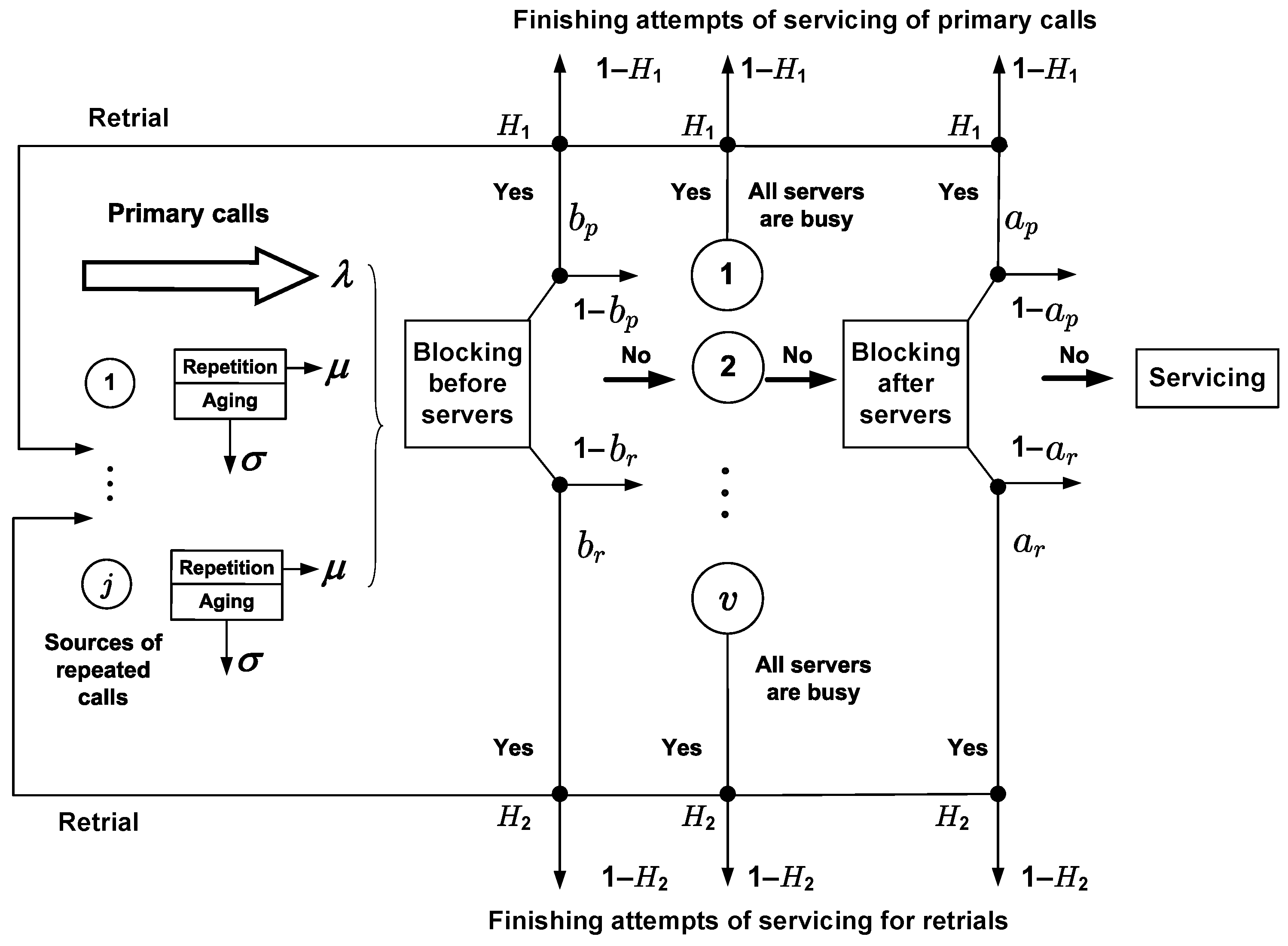
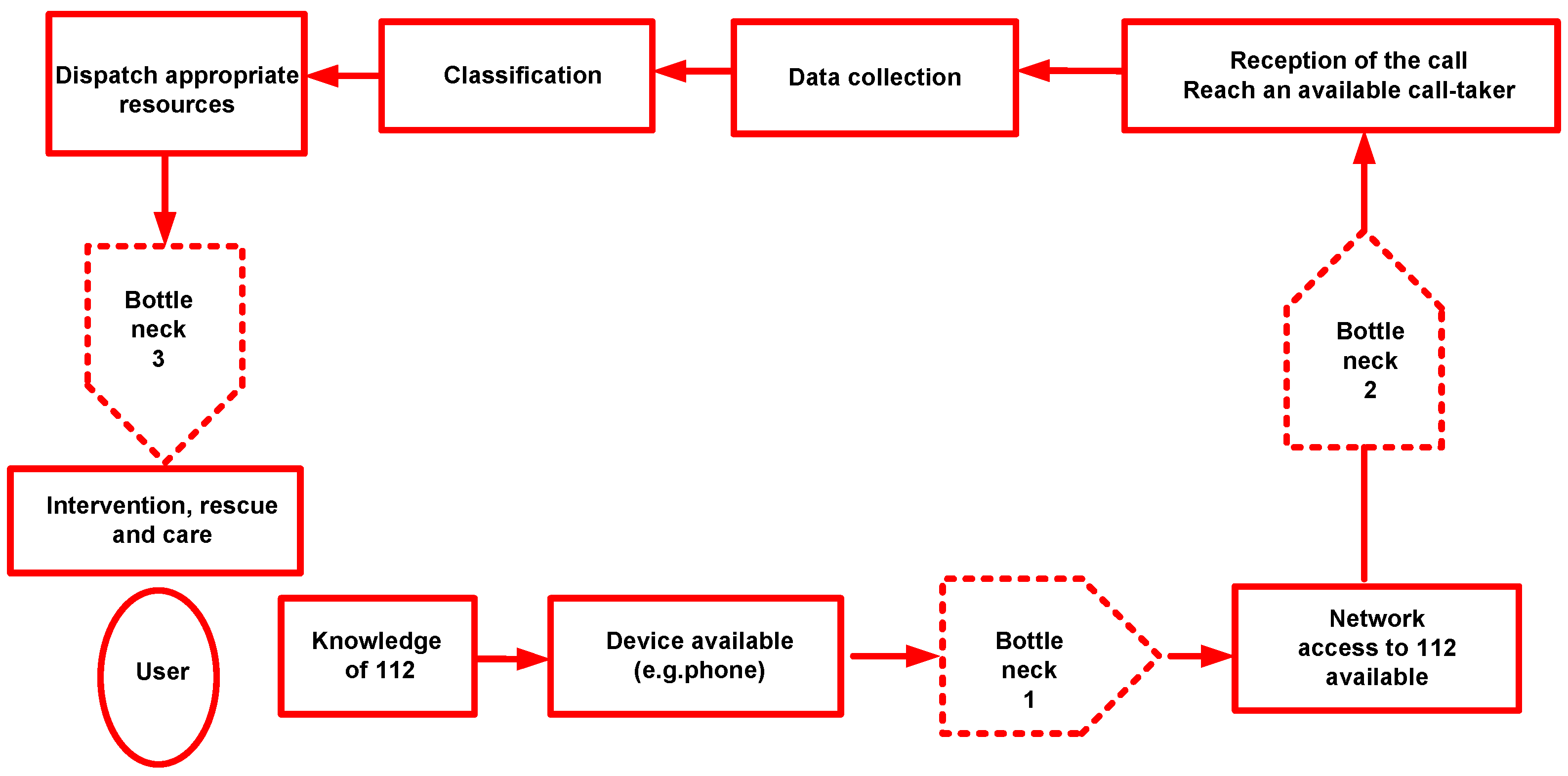
A major part of the existing research suggests that the reason for call repetition is strictly connected to occupancy of the servers and does not take into account the possibility of blocking and subsequent call repetition before and after occupation of the free server. However, there exist a lot of situations where this peculiarity of input flow formation should be taken into account. For example, in an emergency service, a customer can repeat an attempt after being processed by IVR (Interactive Voice Response) or can be blocked on route to the emergency service. This happens before the occupation of a free operator. The operator can refuse to service a call, and become the reason for retrial because of restricted access to the intervention resources required for proper call servicing. This happens in the presence of a free operator. The listed sequence of bottlenecks occurs in the emergency service chain; see Figure 1 taken from [1]. The same types of blocking should be considered when we model transmission resource occupancy in routes consisting of several links and take into account the possibility of call repetitions because the called party is busy or there is no answer.

Detailed surveys of publications devoted to queueing systems with retrials have been undertaken, e.g., in [14,15,16,17]. By taking into account customer behavior, we can model the input flow in a way that is close to the real processes happening in telecommunication systems that is considered in the overload situation. This aspect creates problems with the theoretical analysis of such models, because time intervals between successive call arrivals are now dependent random variables. We can avoid this problem by including the number of repeated customers in the definition of the model’s state. This is done in most publications devoted to this subject. It allows use of Markov processes for model description but seriously complicates the numerical analysis. Performance measures can be found by solving the system of state equations either using the Gauss–Seidel iterative algorithm [2,18,19,20] or by matrix-geometric methods, when the corresponding Markov process has a suitable structure [17,21,22]. The first approach is time-consuming, and the last is numerically unstable for real values of input parameters because of the necessity to convert a large matrix. Such a situation seriously complicates the use of models with retrials as a component of planning tools, because it requires first numerical stability of the calculation algorithm, and second the possibility to estimate performance measures for any choice of input parameters for a reasonable time.

A model with such characteristics can be found in the literature (see, for example [20]). This is a Markov model of a fully available group of servers with the possibility of call repetition only because all servers are busy. Furthermore, we refer to this model as a basic model with repeated calls. Performance measures of this model can be found using a recursive algorithm based on the concept of truncation of the model’s state space [2,17,19,20,23]. For this model, the asymptotic formulae for the calculation of characteristics in the case of extreme load can be also found in explicit form [24]. We generalize the basic model in three directions. First, we will take into account the possibility of the aging of transmitted information during the process of repetitions. Second, we will consider the scenario of blocking before occupying a server, and third, the possibility of losses after occupying a server. In the last two cases a customer can repeat an attempt. The aim of this paper is to show that performance measures of a generalized model can be calculated with the help of a basic model with some changes in input parameters.

The closest model with retrials to the model considered in this paper was analyzed in [2,19]. That model consists of a fully available group of servers with the possibility of waiting. For this model, asymptotic expressions of performance measures for large loads are derived. The values of the characteristics are obtained after solving the system of state equations by the Gauss–Seidel iterative algorithm. The distinguishing features of the model and results obtained in this paper, compared to [2,19], are as follows:

• Additional features, such as the possibility of blocking and call repetition after occupying the server, and the possibility of the aging of transmitted information, are considered.
• Performance measures are calculated using a recursive algorithm without construction of the sequence of approximations such as in the realization of the Gauss–Seidel procedure. This significantly reduces the counting time.

A short outline of this paper is as follows. In Section 2, the mathematical description of the basic model with retrials is presented. In Section 3, the same is done for the considered generalized model with retrials. The possibility of using the basic model for the calculation of performance measures of the generalized model is shown by the construction of some number of auxiliary models. That mathematical analysis is presented in Section 4. Section 5 contains the numerical results that show the possibility of using the analyzed model for the elimination of negative effects from PSAP overload based on filtration of the input flow of calls. Section 6 concludes the paper. 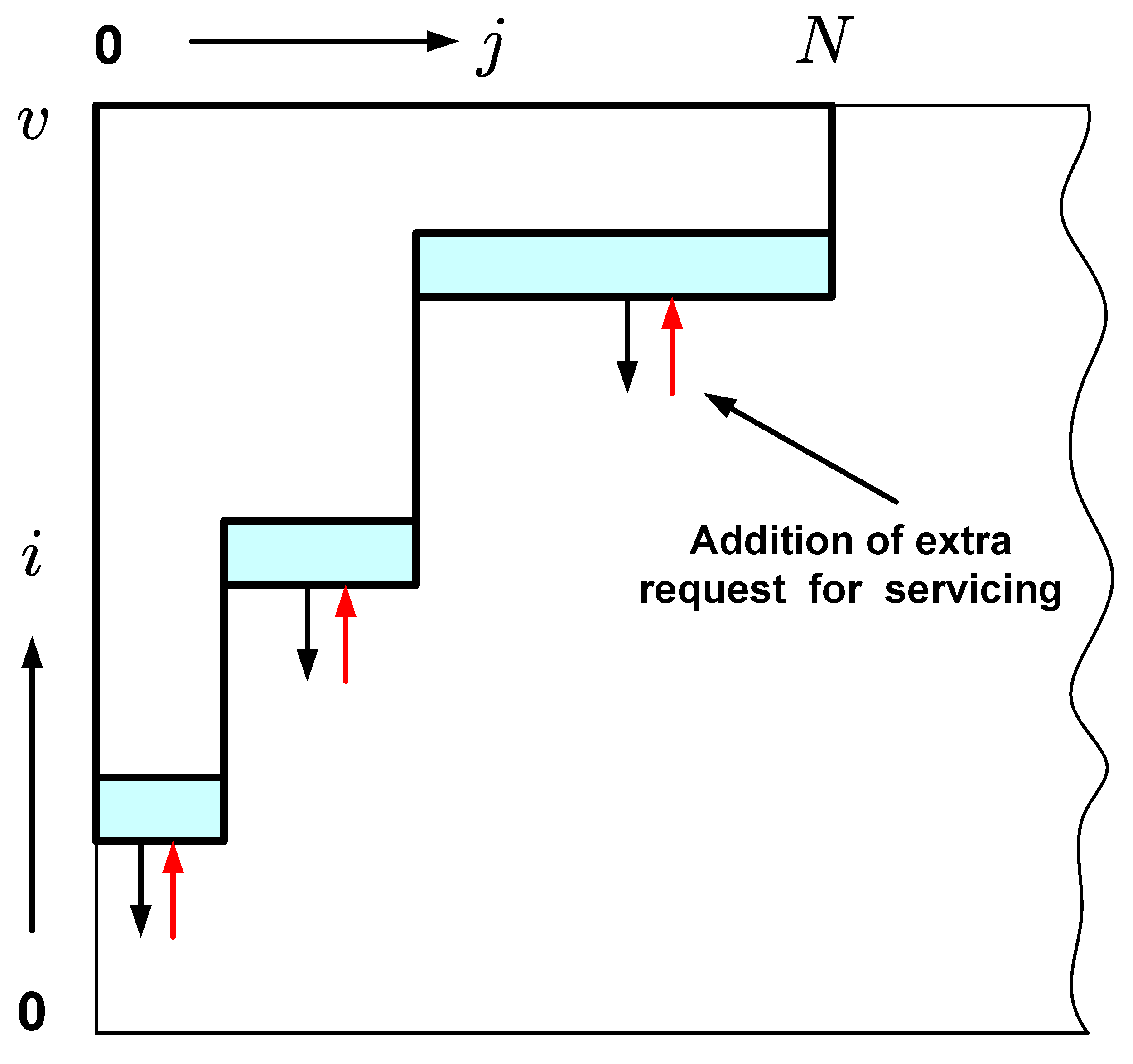The Appendix A contains a brief description of the recursive algorithm that allows the estimation of the performance measures of the basic model using an approach based on the concept of truncated state space.

The novelty of the results obtained in this work is as follows:

• A new model for the functioning of a group of serving devices (servers) has been built and investigated, in which the user can additionally receive a refusal and repeat the call before and after seizing the server. It is also possible for transmitted information to age for the user repeating the call. The model can be used for the elimination of negative effects of overload in various telecommunication systems such as emergency information services, call and contact centers, access nodes, etc.
• A procedure for transforming the model under study has been developed, which makes it possible to exclude the reasons for repeating a call before and after occupation of the server and the possibility of the aging of transmitted information. Thus, the calculation of the model is reduced to the calculation of the characteristics of its particular case, with the only reason for the denial of service being the busyness of the servers. This problem is much easier to solve using an approach based on the concept of a truncated state space. This method of performance measurement estimation allows significant savings of computer resources to be made by ignoring highly unlikely states in the process of calculation.

2. Basic Model Description

The basic model consists of a fully available group of v servers with incoming Poisson flow of primary call intensity $\lambda$. After being refused servicing, a customer makes another attempt to obtain the free server in a random time with probability $H_1$ for a primary call and with probability $H_2$ for a repeated call, exponentially distributed with parameter $\mu$, and, with additional probability, respectively, $1-H_1$, and $1-H_2$, the customer stops their attempts to obtain a connection and leaves the system. Without loss of generality, we can suppose that the service time of a call (primary or repeated) is exponentially distributed with parameter equal to one, and it does not depend on the type of a call. It should be noted that the Poisson model is used only for the construction of the flow of primary calls. The total flow of requests for servicing includes repeated calls, and does not follow the Poisson model. This flow is quite complicated. It reflects the quality of application service that has been observed in the past. The possibility of using Poisson model is also discussed in the Introduction section.

Let us denote by $j\left(t\right)$ the number of repeating customers and by $i\left(t\right)$ the number of busy servers at time t. The model’s functioning is described by a two-dimensional Markov process $r\left(t\right)=\left(j\right(t),i(t\left)\right)$ with an infinite number of states S, $(j,i)\in S$, $j=0,1,\dots ,i=0,1,\dots ,v$. Let us denote by $P(j,i)$ the probability of stationary state $(j,i)$ of $r\left(t\right)$. Here, j is the number of repeating customers and i is the number of busy servers. Using the ideas of [25] it can be proved that stationary distribution for $r\left(t\right)$ exists if $\mu >0$ and $H_2<1$. If $H_2=1$, parameters $\lambda$ and $\mu$ should satisfy the inequalities $\lambda H_1<v$ and $\mu >0$. The values of $P(j,i)$ can be found after solving of the following system of state equations:

$$\begin{array}{cc}\hfill P(j,v)& \left(\lambda H_1+j\mu (1-H_2)+v\right)=P(j,v-1)\lambda +P(j-1,v)\lambda H_1+\hfill \\ \hfill & P(j+1,v-1)(j+1)\mu +P(j+1,v)(j+1)\mu (1-H_2),\hfill \\ \hfill & j=0,1,\dots ,i=v;\hfill \\ \hfill P(j,i)& \left(\lambda +j\mu +i\right)=P(j,i-1)\lambda +P(j+1,i-1)(j+1)\mu +\hfill \\ \hfill & P(j,i+1)(i+1),j=0,1,\dots ,i=0,1,\dots v-1.\hfill \end{array}$$

(1)

The normalizing condition is held for $P(j,i)$. Here and beyond, we suppose that in the system of state equations, the probability of state with negative-integer components is equal to zero. Let us introduce the following notations:

$$P\left(i\right)=\sum _{j=0}^{\infty }P(j,i),J\left(i\right)=\sum _{j=0}^{\infty }P(j,i)j,i=0,1,\dots ,v.$$

In this paper we are using a standard family of performance measures that can be defined for the model with repeated attempts using stationary probabilities of the Markov process that describes model functioning. All such, characteristics can be expressed through $P\left(i\right)$ and $J\left(i\right)$. For example, the value of I is the mean number of busy servers, the value of J is the mean number of repeating customers, the value of ${\pi }_c$ is the ratio of lost calls, the value of $\tau$ is the ratio of repeated attempts in the total flow of incoming calls, and the value of M is the mean number of retrials per one primary call can be found from expressions

$$\begin{array}{cc}\hfill & I=\sum _{i=0}^{v}P\left(i\right)i,J=\sum _{i=0}^{v}J\left(i\right),{\pi }_c=\frac{\lambda p\left(v\right)+J\left(v\right)\mu }{\lambda +J\mu },\hfill \\ \hfill & \tau =\frac{J\mu }{\lambda +J\mu },M=\frac{J\mu }{\lambda }.\hfill \end{array}$$

(2)

Considering this further we will work only with $P\left(i\right)$ and $J\left(i\right)$ and call these characteristics basic. Summing up the system of state Equation (1) over j with i fixes, we obtain the local conservation laws for macrostate $\left(i\right)$

$$P\left(i\right)\lambda +J\left(i\right)\mu =P(i+1)(i+1),i=0,1,\dots ,v-1.$$

(3)

Summing up the system of state Equation (1) over i with j fixes, we obtain the similar relationships for macrostate $\left(j\right)$

$$\begin{array}{cc}\hfill P(j,v)& \lambda H_1=P(j+1,v)(j+1)\mu (1-H_2)+\sum _{i=0}^{v-1}P(j+1,i)(j+1)\mu ,\hfill \\ \hfill & j=0,1,\dots \hfill \end{array}$$

(4)

Summing up (3) and (4) over i and j, we obtain the conservation laws that relate main stationary characteristics of the basic model

$$\lambda (1-P\left(v\right))+(J-J\left(v\right))\mu =I,J\mu =\lambda P\left(v\right)H_1+J\left(v\right)\mu H_2.$$

(5)

Relationship (5) can be used for the estimation of the error caused by truncation of the used state space (see Appendix A), for the indirect measurement of the intensity of primary calls and for solving a variety of other problems arising in the exact and approximate analysis of the introduced model [2,18,19,20]. To find $P\left(i\right)$ and $J\left(i\right)$, it is necessary to solve the system of state Equation (1). The numerical procedure of doing this is briefly described in Appendix A. In more detail, this approach is presented in [20] for the particular case of the studied model, when $H_1=H_2=H$. An elaborated calculation method is based on the concept of truncated state space. This approach allows significant savings of computer resources to be made by ignoring highly unlikely states in the process of calculation. The numerical procedure includes two steps: first, it is necessary to decrease the number of unknowns in the system of state equations by not considering the states with negligible probabilities of existence. Second, it is necessary to find the error of estimation of the performance measures caused by truncation.

3. Generalized Model Description

We generalize the introduced model in the following three directions.

(1)

We take into account the possibility of aging transmitted information during the process of repetitions. This situation can be modeled in the following way. We suppose that starting the process of repetitions also starts the process of aging. The maximum allowed time of aging is exponentially distributed with parameter $\sigma$. After this time, the customer stops the process of repetitions and leaves the system, unserved.

(2)

We also consider the opportunity of losses before occupying the server. This situation will be modeled in the following way. We suppose that incoming call with probability $b_p$ for primary call and with probability $b_r$ for repeated call can be blocked before entering the service system. In this case, with probability $H_1$ for primary call and with probability $H_2$ for repeated call, the customer repeats the attempt after a random time, exponentially distributed with parameter $\mu$, and with additional probabilities, respectively, $1-H_1$, and $1-H_2$, the customer stops attempting to obtain a connection and leaves the system, unserved. The probabilities $b_p$ and $b_r$ can be interpreted as losses at the stage of obtaining service between customer and the service system.

(3)

In the same way, we take into account the possibility of losses after the occupation of the server. The probabilities of this event are $a_p$ for a primary call and $a_r$ for a repeated call. Probabilities of repetitions are, respectively, $H_1$ and $H_2$ for primary and repeated attempts. Time between successive repeated attempts in this case is also exponentially distributed with parameter $\mu$. The probabilities of losses $a_p$ and $a_r$ can be interpreted as losses at the stages of servicing between service system and additional resources required for proper call servicing.

The basic model is a particular case of the generalized model. We obtain it by choosing $b_p=b_r=a_p=a_r=\sigma =0$. To simplify the notation, we will use for performance measures of the generalized model the same symbols that were used for corresponding characteristics of the basic model. Different values of probabilities of losses for primary and repeated calls allow consideration of the following property of functioning of the service systems in overload conditions. After being refused service with some probability in primary attempt, a customer making repeated attempts will obtain a refusal with greater probability. The functional model of the studied service system is presented in Figure 2.

The model’s functioning is described by a two-dimensional Markov process $r\left(t\right)=\left(j\right(t),i(t\left)\right)$, where $j\left(t\right)$ is the number of repeating customers and $i\left(t\right)$ is the number of busy servers at time t defined in infinite state space S, $(j,i)\in S$, $j=0,1,\dots ,i=0,1,\dots ,v$. To remove out of consideration the exotic cases, we suppose that $b_p<1$, $b_r<1$, $a_p<1$, $a_r<1$. Let us denote by $P(j,i)$ the probability of the stationary state $(j,i)$ of $r\left(t\right)$. Using the ideas of [25] it can be proved that stationary distribution for $r\left(t\right)$ exists if

• $\mu >0$, $\sigma >0$;
• $\mu >0$, $\sigma =0$ but $H_2<1$;
• $\mu >0$, $\sigma =0$, $H_2=1$ but $\lambda H_1<v$.

The values of $P(j,i)$ can be found after solving the following system of state equations:

$$\begin{array}{cc}\hfill P(j,v)& \left(\lambda H_1+j(\sigma +\mu (1-H_2))+v\right)=P(j,v-1)\lambda (1-b_p)(1-a_p)+\hfill \\ \hfill & P(j-1,v)\lambda H_1+P(j+1,v-1)(j+1)\mu (1-b_r)(1-a_r)+\hfill \\ \hfill & P(j+1,v)(j+1)(\sigma +\mu (1-H_2)),j=0,1,\dots ,i=v;\hfill \\ \hfill P(j,i)& \left(\lambda \right(1-(1-H_1)(b_p+(1-b_p)a_p))+\hfill \\ \hfill & j(\sigma +\mu (1-H_2(b_r+(1-b_r)a_r)))+i)=\hfill \\ \hfill & P(j,i-1)\lambda (1-b_p)(1-a_p)+P(j-1,i)\lambda H_1(b_p+(1-b_p)a_p)+\hfill \\ \hfill & P(j+1,i-1)(j+1)\mu (1-b_r)(1-a_r)+\hfill \\ \hfill & P(j+1,i)(j+1)(\sigma +\mu (1-H_2)(b_r+(1-b_r)a_r))+\hfill \\ \hfill & P(j,i+1)(i+1),j=0,1,\dots ,i=0,1,\dots v-1.\hfill \end{array}$$

(6)

The normalizing condition is held for $P(j,i)$. Let us introduce the notations

$$P\left(i\right)=\sum _{j=0}^{\infty }P(j,i),J\left(i\right)=\sum _{j=0}^{\infty }P(j,i)j,i=0,1,\dots ,v.$$

In the same way as was done for the basic model, we can prove that local conservation laws for macrostates $\left(i\right)$ and $\left(j\right)$ are looking as follows:

$$\begin{array}{cc}\hfill & P\left(i\right)\lambda (1-b_p)(1-a_p)+J\left(i\right)\mu (1-b_r)(1-a_r)=P(i+1)(i+1),\hfill \\ \hfill & i=0,1,\dots ,v-1;\hfill \end{array}$$

(7)

$$\begin{array}{cc}\hfill \sum _{i=0}^{v}P(j,i)& \lambda H_1{b}_p+P(j,v)\lambda H_1(1-b_p)+\sum _{i=0}^{v-1}P(j,i)\lambda H_1(1-b_p)a_p=\hfill \\ \hfill & \sum _{i=0}^{v}P(j+1,i)(j+1)\left(\sigma +\mu b_r(1-H_2)\right)+\hfill \\ \hfill & P(j+1,v)(j+1)\mu (1-b_r)(1-H_2)+\hfill \\ \hfill & \sum _{i=0}^{v-1}P(j+1,i)(j+1)\mu (1-b_r)(1-a_r{H}_2),j=0,1,\dots \hfill \end{array}$$

(8)

If values of $P\left(i\right)$ and $J\left(i\right)$ are known, we can calculate the main stationary characteristics of the model. For example, the corresponding formulae for I, J, ${\pi }_c$, $\tau$ and M can be found from expressions (see (2))

$$\begin{array}{cc}\hfill & I=\sum _{i=0}^{v}P\left(i\right)i,J=\sum _{i=0}^{v}J\left(i\right),{\pi }_c=\frac{\lambda B_p+B_r\mu +J\sigma }{\lambda +J\mu },\hfill \\ \hfill & \tau =\frac{J\mu }{\lambda +J\mu },M=\frac{J\mu }{\lambda },\hfill \end{array}$$

(9)

where

$$\begin{array}{cc}\hfill & B_p=b_p+(1-b_p)P\left(v\right)+(1-b_p)(1-P\left(v\right))a_p,\hfill \\ \hfill & B_r=J{b}_r+J\left(v\right)(1-b_r)+(J-J\left(v\right))(1-b_r)a_r.\hfill \end{array}$$

Summing up (7) and (8) over i and j, we obtain the conservation laws that relate to the main stationary characteristics of the generalized model

$$\begin{array}{cc}\hfill & \lambda (1-P\left(v\right))(1-b_p)(1-a_p)+(J-J\left(v\right))(1-b_r)(1-a_r)\mu =I,\hfill \\ \hfill & J(\mu +\sigma )=\lambda B_p{H}_1+B_r\mu H_2.\hfill \end{array}$$

(10)

As we can see from the above expressions, all stationary performance measures of the generalized model can be defined through $P\left(i\right)$ and $J\left(i\right)$, $i=0,1,\dots ,v$. To calculate the values of $P\left(i\right)$ and $J\left(i\right)$, it is necessary to solve the system of state Equation (6). We are not able to find the values of $P(j,i)$ recursively as can be done for the basic model (see Appendix A), because in the generalized model a customer can repeat an attempt for any state of busy servers $i=0,1,\dots ,v$. In the basic model, this can be done only when $i=v$. What remains is the solving of (6) by standard approaches, either by Gauss–Seidel iterative algorithm or by matrix-geometric methods. The first approach is time-consuming; the last is numerically unstable for real values of input parameters, because of the necessity to convert a large matrix. We overcome these difficulties by showing that values of $P\left(i\right)$ and $J\left(i\right)$ can be calculated with the help of the corresponding characteristics of the basic model after a suitable choice of values of its input parameters. We prove it by constructing the number of auxiliary models using another probabilistic interpretation of input parameters of the generalized model or by algebraic transformations of the system of state equations.

All four auxiliary models that will appear later (the last is a basic model) will be particular cases of the generalized model, so we can use the same symbols to denote its input parameters and characteristics, differing them only by a superscript. The value of the digit used in the superscript for performance measures $P\left(i\right)$ and $J\left(i\right)$ means the number of auxiliary model. For input parameters, the digit denotes the number, changing by parameter its value. A parameter without a superscript has the same value as the generalized model.

4. Auxiliary Models

4.1. First Auxiliary Model

The process of call repetition and the aging of transmitted information can be represented in the following way. Let us consider some refusal. If such an event happens, a customer, with probabilities $H_x$ ($x=1,2$, depending on the number of attempt), makes another call after a random time $T_{\mu }$ with exponential distribution with parameter $\mu$ or, with probabilities $1-H_x$, stops attempts to obtain service. If refusal in service was obtained for primary calls, then the random time $T_{\sigma }$ of aging of the transmitted information for the considered customer starts at the moment of call repetition. The value of $T_{\sigma }$ has exponential distribution with parameter $\sigma$ and does not depend on other exponentially distributed variables realized in the model. If the refusal in servicing was obtained in repeated attempts, then, starting from the moment of call repetition, the remaining time of aging also has exponential distribution with parameter $\sigma$ and does not depend on other exponentially distributed variables realized in the model. This result follows from the basic property of exponentially distributed random variables.

By considering the above-stated argument, we can remodel the process of call repetition and aging of transmitted information in the following way. After refusal of service, a customer with probability $H_x$ stays in the system for a random time equal to $min(T_{\mu },T_{\sigma })$ with exponential distribution with parameter $\mu +\sigma$. Then, with probability of event $T_{\mu }>T_{\sigma }$ equal to $\frac{\sigma }{\mu +\sigma }$, at the end of this time a customer leaves the system because of the aging of transmitted information and with the probability of event $T_{\mu }<T_{\sigma }$ equal to $\frac{\mu }{\mu +\sigma }$ a customer makes a repeated attempt. The fact that with some known probability the customer stays in the system without subsequent call repetition and then leaves the system does not influence the process of server occupation.

Let us construct the first auxiliary model by making the following changes in the generalized model. We suppose that after being refused, a customer with probability $\frac{H_x\mu }{\mu +\sigma }$ makes another attempt in a time interval with exponential distribution with parameter $\mu +\sigma$, and with additional probability $1-\frac{H_x\mu }{\mu +\sigma }$ the customer immediately leaves the system. It is easy to notice that the first auxiliary model is a particular case of the generalized model. We obtain it by choosing in the generalized model the following values of input parameters:

$$H_1^{\left(1\right)}=\frac{H_1\mu }{\mu +\sigma },H_2^{\left(1\right)}=\frac{H_2\mu }{\mu +\sigma },{\mu }^{\left(1\right)}=\mu +\sigma ,{\sigma }^{\left(1\right)}=0.$$

(11)

Other parameters remain the same as in the generalized model. From the above considerations (7) and (12), we can conclude that the following relations are true:

$$P\left(i\right)=P^{\left(1\right)}\left(i\right),J\left(i\right)=J^{\left(1\right)}\left(i\right)\frac{\mu +\sigma }{\mu },,i=0,1,\dots ,v,$$

(12)

where

$$P^{\left(1\right)}\left(i\right)=\sum _{j=0}^{\infty }{P}^{\left(1\right)}(j,i),J^{\left(1\right)}\left(i\right)=\sum _{j=0}^{\infty }{P}^{\left(1\right)}(j,i)j,i=0,1,\dots ,v$$

and $P^{\left(1\right)}(j,i)$ are the stationary probabilities of state $(j,i)$ of a Markov process that describes the functioning of the first auxiliary model. Relationship (12) for particular cases of the basic model was also proven in [26,27] by algebraic transformations of the system of state equations. Let us consider the first auxiliary model and continue the process of its simplification.

4.2. Second Auxiliary Model

All input parameters of this model have the same values as the corresponding parameters of the first auxiliary model. We only divide the repeating customers into two groups. In the first group, the number of repeating customers increases by one with probability $H_1^{\left(1\right)}(b_p+(1-b_p)a_p)$ each time when the primary call appears in the first auxiliary model. The repeating customer of this group leaves the group with probability $1-H_2^{\left(1\right)}(b_r+(1-b_r)a_r)$ after a random time with exponential distribution with parameter $\mu$ and with additional probability of continuing to stay in the first group.

Please note that increasing and decreasing of the number of repeating customers in the first group happens with the same probabilities for all possible values of busy servers. We put all other repeating subscribers of first auxiliary model in the second group. After leaving the first group, a customer can occupy the server, move to the second group of repeating customers, or stop attempts for service. Otherwise, the functioning of a new auxiliary model does not change compared to the first auxiliary model. A more detailed description of the changing of the states of the second auxiliary model can be seen from the system of state Equation (13) that will appear below.

Let us denote by $j_1\left(t\right)$ and $j_2\left(t\right)$ the number of repeating customers at time t in the first and second groups, respectively, and by $i\left(t\right)$ we denote the number of busy servers at time t. The dynamic of changing the model states is described by a three-dimensional Markov process of the type $r\left(t\right)=(j_1\left(t\right),j_2\left(t\right),i\left(t\right))$ with infinite number of states S, $(j_1,j_2,i)\in S$, $j_1=0,1,\dots ,j_2=0,1,\dots ,i=0,1,\dots ,v$. Let us denote by $P^{\left(2\right)}(j_1,j_2,i)$ the probability of stationary state $(j_1,j_2,i)$ of $r\left(t\right)$. The system of state equations can be written in the following way

$$\begin{array}{cc}\hfill P^{\left(2\right)}(j_1,j_2,v)& \left(\lambda H_1^{\left(1\right)}+j_1{\mu }^{\left(1\right)}(1-H_2^{\left(1\right)}(b_r+(1-b_r)a_r))+j_2{\mu }^{\left(1\right)}(1-H_2^{\left(1\right)})+v\right)=\hfill \\ \hfill & P^{\left(2\right)}(j_1,j_2,v-1)\lambda (1-b_p)(1-a_p)+\hfill \\ \hfill & P^{\left(2\right)}(j_1-1,j_2,v)\lambda H_1^{\left(1\right)}(b_p+(1-b_p)a_p)+\hfill \\ \hfill & P^{\left(2\right)}(j_1,j_2-1,v)\lambda H_1^{\left(1\right)}(1-b_p)(1-a_p)+\hfill \\ \hfill & P^{\left(2\right)}(j_1+1,j_2,v-1)(j_1+1){\mu }^{\left(1\right)}(1-b_r)(1-a_r)+\hfill \\ \hfill & P^{\left(2\right)}(j_1+1,j_2,v)(j_1+1){\mu }^{\left(1\right)}(1-H_2^{\left(1\right)})+\hfill \\ \hfill & P^{\left(2\right)}(j_1+1,j_2-1,v)(j_1+1){\mu }^{\left(1\right)}{H}_2^{\left(1\right)}(1-b_r)(1-a_r)+\hfill \\ \hfill & P^{\left(2\right)}(j_1,j_2+1,v-1)(j_2+1){\mu }^{\left(1\right)}(1-b_r)(1-a_r)+\hfill \\ \hfill & P^{\left(2\right)}(j_1,j_2+1,v)(j_2+1){\mu }^{\left(1\right)}(1-H_2^{\left(1\right)}),\hfill \\ \hfill & j_1=0,1,\dots ,j_2=0,1,\dots ,i=v;\hfill \end{array}$$

(13)

$$\begin{array}{cc}\hfill P^{\left(2\right)}(j_1,j_2,i)& (\lambda (1-(1-H_1^{\left(1\right)})(b_p+(1-b_p)a_p))+j_1{\mu }^{\left(1\right)}(1-H_2^{\left(1\right)}(b_r+(1-b_r)a_r))+\hfill \\ \hfill & j_2{\mu }^{\left(1\right)}(1-H_2^{\left(1\right)}(b_r+(1-b_r)a_r))+i)=\hfill \\ \hfill & P^{\left(2\right)}(j_1,j_2,i-1)\lambda (1-b_p)(1-a_p)+\hfill \\ \hfill & P^{\left(2\right)}(j_1-1,j_2,i)\lambda H_1^{\left(1\right)}(b_p+(1-b_p)a_p)+\hfill \\ \hfill & P^{\left(2\right)}(j_1+1,j_2,i-1)(j_1+1){\mu }^{\left(1\right)}(1-b_r)(1-a_r)+\hfill \\ \hfill & P^{\left(2\right)}(j_1+1,j_2,i)(j_1+1){\mu }^{\left(1\right)}(1-H_2^{\left(1\right)})(b_r+(1-b_r)a_r)+\hfill \\ \hfill & P^{\left(2\right)}(j_1,j_2+1,i-1)(j_2+1){\mu }^{\left(1\right)}(1-b_r)(1-a_r)+\hfill \\ \hfill & P^{\left(2\right)}(j_1,j_2+1,i)(j_2+1){\mu }^{\left(1\right)}(1-H_2^{\left(1\right)})(b_r+(1-b_r)a_r)+\hfill \\ \hfill & P^{\left(2\right)}(j_1,j_2,i+1)(i+1),\hfill \\ \hfill & j_1=0,1,\dots ,j_2=0,1,\dots ,i=0,1,\dots ,v-1.\hfill \end{array}$$

The normalization condition is held for $P^{\left(2\right)}(j_1,j_2,i)$. The input parameters of the first and the second auxiliary models are the same. The process of call repetition and server occupation is the same. We only introduce the rule of separating the repeating customers into two groups. As result, between the corresponding characteristics of the first and the second auxiliary models the following relations are valid:

$$P^{\left(1\right)}\left(i\right)=P^{\left(2\right)}\left(i\right),J^{\left(1\right)}\left(i\right)=J_1^{\left(2\right)}\left(i\right)+J_2^{\left(2\right)}\left(i\right)=J^{\left(2\right)}\left(i\right),i=0,1,\dots ,v,$$

(14)

where

$$\begin{array}{cc}\hfill & P^{\left(2\right)}\left(i\right)=\sum _{j_1=0}^{\infty }\sum _{j_2=0}^{\infty }{P}^{\left(2\right)}(j_1,j_2,i),J_1^{\left(2\right)}\left(i\right)=\sum _{j_1=0}^{\infty }\sum _{j_2=0}^{\infty }{P}^{\left(2\right)}(j_1,j_2,i)j_1,\hfill \\ \hfill & J_2^{\left(2\right)}\left(i\right)=\sum _{j_1=0}^{\infty }\sum _{j_2=0}^{\infty }{P}^{\left(2\right)}(j_1,j_2,i)j_2,i=0,1,\dots ,v.\hfill \end{array}$$

4.3. Third Auxiliary Model

Let us show that the solution of (13) can be represented in the form

$$\begin{array}{cc}\hfill P^{\left(2\right)}(j_1,j_2,i)& =P^{\left(2\right)}(0,j_2,i)\frac{D^{j_1}}{j_1!},j_1=0,1,\dots ,\hfill \\ \hfill & (j_1,j_2,i)\in S,\hfill \end{array}$$

(15)

where

$$D=\frac{\lambda H_1^{\left(1\right)}(b_p+(1-b_p)a_p)}{{\mu }^{\left(1\right)}\left(1-H_2^{\left(1\right)}(b_r+(1-b_r)a_r)\right)}.$$

After the substitution of (15) into (13) with changing $P^{\left(2\right)}(0,j_2,i)$ into $P^{\left(3\right)}(j,i)$, we obtain the following system of linear equations

$$\begin{array}{cc}\hfill P^{\left(3\right)}(j,v)& \left({\lambda }^{\left(1\right)}{H}_1^{\left(2\right)}+j({\mu }^{\left(2\right)}(1-H_2^{\left(1\right)})+{\sigma }^{\left(1\right)})+v\right)=P^{\left(3\right)}(j,v-1){\lambda }^{\left(1\right)}+\hfill \\ \hfill & P^{\left(3\right)}(j-1,v){\lambda }^{\left(1\right)}{H}_1^{\left(2\right)}+P^{\left(3\right)}(j+1,v-1)(j+1){\mu }^{\left(2\right)}+\hfill \\ \hfill & +P^{\left(3\right)}(j+1,v)(j+1)({\mu }^{\left(2\right)}(1-H_2^{\left(1\right)})+{\sigma }^{\left(1\right)}),\hfill \\ \hfill & j=0,1,\dots ,i=v;\hfill \end{array}$$

(16)

$$\begin{array}{cc}\hfill P^{\left(3\right)}(j,i)& \left({\lambda }^{\left(1\right)}+j({\mu }^{\left(2\right)}+{\sigma }^{\left(1\right)})+i\right)=P^{\left(3\right)}(j,i-1){\lambda }^{\left(1\right)}+P^{\left(3\right)}(j+1,i-1)(j+1){\mu }^{\left(2\right)}+\hfill \\ \hfill & P^{\left(3\right)}(j+1,i)(j+1){\sigma }^{\left(1\right)}+P^{\left(3\right)}(j,i+1)(i+1),\hfill \\ \hfill & j=0,1,\dots ,i=0,1,\dots v-1,\hfill \end{array}$$

where

$$\begin{array}{cc}\hfill & {\lambda }^{\left(1\right)}=\lambda \left((1-b_p)(1-a_p)+(1-b_r)(1-a_r)A\right),\hfill \\ \hfill & A=\frac{H_1^{\left(1\right)}(b_p+(1-b_p)a_p)}{1-H_2^{\left(1\right)}(b_r+(1-b_r)a_r)},\hfill \\ \hfill & {\mu }^{\left(2\right)}={\mu }^{\left(1\right)}(1-b_r)(1-a_r),\hfill \\ \hfill & {\sigma }^{\left(1\right)}={\mu }^{\left(1\right)}(1-H_2^{\left(1\right)})(b_r+(1-b_r)a_r),\hfill \\ \hfill & H_1^{\left(2\right)}=\frac{(1-b_p)(1-a_p)H_1^{\left(1\right)}+(1-b_r)(1-a_r)H_2^{\left(1\right)}A}{(1-b_p)(1-a_p)+(1-b_r)(1-a_r)A}.\hfill \end{array}$$

(17)

Because $H_1^{\left(2\right)}\le 1$ and $H_2^{\left(1\right)}\le 1$ then we can conclude that the system of linear Equation (16) will be the system of state Equation (6) of a particular case of generalized model with the choice of blocking probabilities before and after the group of v servers in the form $b_p^{\left(1\right)}=b_r^{\left(1\right)}=a_p^{\left(1\right)}=a_r^{\left(1\right)}=0$ and other parameters defined by (11) and (17). Provided that the ergodicity properties hold for Markov process $r\left(t\right)$ describing the generalized model, the system of state Equation (16) has a unique solution and the solution of (13) has the form (15). Let us call the constructed particular case of generalized model as the third auxiliary model. From (15) we follow the relationship between corresponding characteristics of the second and the third auxiliary models

$$P^{\left(2\right)}\left(i\right)=P^{\left(3\right)}\left(i\right),J^{\left(2\right)}\left(i\right)=J^{\left(3\right)}\left(i\right)+D{P}^{\left(3\right)}\left(i\right),i=0,1,\dots ,v,$$

(18)

where

$$P^{\left(3\right)}\left(i\right)=\sum _{j=0}^{\infty }{P}^{\left(3\right)}(j,i),J^{\left(3\right)}\left(i\right)=\sum _{j=0}^{\infty }{P}^{\left(3\right)}(j,i)j,i=0,1,\dots ,v.$$

4.4. Fourth Auxiliary Model

The last step in constructing a basic model is to eliminate the event of aging of the transmitted information from the third auxiliary model. The eliminated event is described by a random time with an exponential distribution with parameter ${\sigma }^{\left(1\right)}$. We have already discovered how to solve this problem when analyzing the first auxiliary model (see, Section 4.1). According to these results, the fourth auxiliary model is a particular case of the generalized model with the following choice of input parameters

$$\begin{array}{cc}\hfill & {\lambda }^{\left(1\right)}=\lambda \left((1-b_p)(1-a_p)+(1-b_r)(1-a_r)A\right),\hfill \\ \hfill & {\mu }^{\left(3\right)}={\mu }^{\left(2\right)}+{\sigma }^{\left(1\right)},\hfill \\ \hfill & {\sigma }^{\left(2\right)}=b_p^{\left(1\right)}=b_r^{\left(1\right)}=a_p^{\left(1\right)}=a_r^{\left(1\right)}=0,\hfill \\ \hfill & H_1^{\left(3\right)}=H_1^{\left(2\right)}\frac{{\mu }^{\left(2\right)}}{{\mu }^{\left(2\right)}+{\sigma }^{\left(1\right)}},\hfill \\ \hfill & H_2^{\left(2\right)}=H_2^{\left(1\right)}\frac{{\mu }^{\left(2\right)}}{{\mu }^{\left(2\right)}+{\sigma }^{\left(1\right)}}.\hfill \end{array}$$

(19)

This choice of parameters tells us that the fourth auxiliary model is equivalent to the basic model. Similar to the (12), we obtain the relationship between basic characteristics of the third and fourth auxiliary models

$$P^{\left(3\right)}\left(i\right)=P^{\left(4\right)}\left(i\right),J^{\left(3\right)}\left(i\right)=J^{\left(4\right)}\left(i\right)\frac{{\mu }^{\left(2\right)}+{\sigma }^{\left(1\right)}}{{\mu }^{\left(2\right)}},i=0,1,\dots ,v,$$

(20)

where

$$P^{\left(4\right)}\left(i\right)=\sum _{j=0}^{\infty }{P}^{\left(4\right)}(j,i),J^{\left(4\right)}\left(i\right)=\sum _{j=0}^{\infty }{P}^{\left(4\right)}(j,i)j,i=0,1,\dots ,v$$

and $P^{\left(4\right)}(j,i)$ are stationary probabilities of states $(j,i)$ of Markov process that describes the functioning of the fourth auxiliary model that is equivalent to the basic model.

Final expressions for input parameters of the equivalent basic model through parameters of the generalized model are

$$\begin{array}{cc}\hfill & {\lambda }^{\left(1\right)}=\lambda \left((1-b_p)(1-a_p)+(1-b_r)(1-a_r)A\right),\hfill \\ \hfill & A=\frac{H_1\mu \left(b_p+(1-b_p)a_p\right)}{\sigma +\mu \left(1-H_2(b_r+(1-b_r)a_r)\right)},\hfill \\ \hfill & {\mu }^{\left(3\right)}=\sigma +\mu \left(1-H_2(b_r+(1-b_r)a_r)\right),\hfill \\ \hfill & H_1^{\left(3\right)}=\frac{(1-b_p)(1-a_p)H_1+(1-b_r)(1-a_r)H_{2}A}{(1-b_p)(1-a_p)+(1-b_r)(1-a_r)A}\times \hfill \\ \hfill & \frac{\mu (1-(b_r+(1-b_r)a_r))}{\sigma +\mu (1-H_2(b_r+(1-b_r)a_r))},\hfill \\ \hfill & H_2^{\left(2\right)}=\frac{H_2\mu \left(1-(b_r+(1-b_r)a_r)\right)}{\sigma +\mu (1-H_2(b_r+(1-b_r)a_r))}.\hfill \end{array}$$

(21)

Using (20) as input parameters of the basic model, we can calculate the characteristics of the generalized model $P\left(i\right),J\left(i\right)$, $i=0,1,\dots ,v$ for a given set of input parameters $\lambda ,b_p,b_r,H_1,H_2,a_p,a_r,\mu ,\sigma$. The final results are as follows:

$$\begin{array}{cc}\hfill & P\left(i\right)=P^{\left(4\right)}\left(i\right),\hfill \\ \hfill & J\left(i\right)=\frac{\sigma +\mu \left(1-H_2(b_r+(1-b_r)a_r)\right)}{\mu (1-b_r)(1-a_r)}{J}^{\left(4\right)}\left(i\right)+\hfill \\ \hfill & \frac{\lambda H_1(b_p+(1-b_p)a_p)}{\sigma +\mu \left(1-H_2(b_r+(1-b_r)a_r)\right)}{P}^{\left(4\right)}\left(i\right),\hfill \\ \hfill & i=0,1,\dots ,v.\hfill \end{array}$$

(22)

5. Numerical Examples

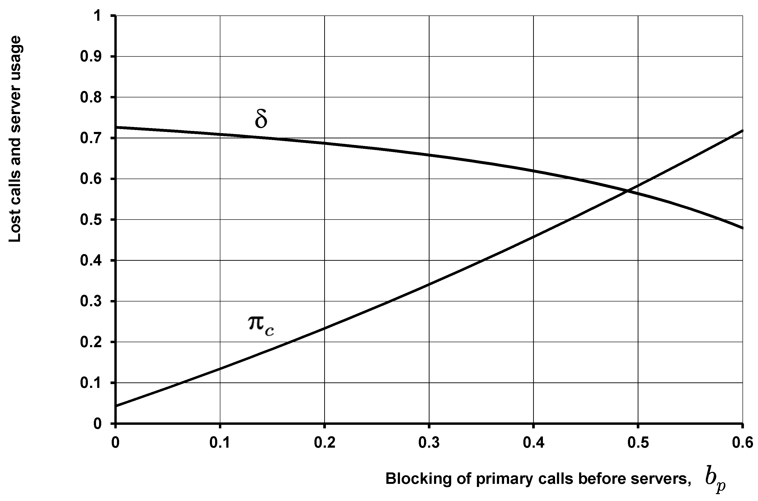
Let us consider a few numerical examples that illustrate the usage of the constructed model for practical purposes. We start by showing the influence of blocking before and after the servers on values of main performance measurements: ${\pi }_c$—the ratio of lost calls—and $\delta =\frac{I}{v}$—the mean value of one server usage. Figure 3 illustrates the dependence of ${\pi }_c$ and $\delta$ on the probability of primary and repeated calls blocking before servers.

The values of $b_p$ are varying in interval from 0 to $0.6$. For fixed $b_p$ the value of $b_r$ is calculated from relationship $b_r=b_p\times 1.3$. Other fixed parameters used for Figure 3 are as follows: $\lambda =22$; $v=30$; $\mu =5$; $H_1=H_2=0.8$; $\sigma =0.2$; $a_p=a_r=0$.

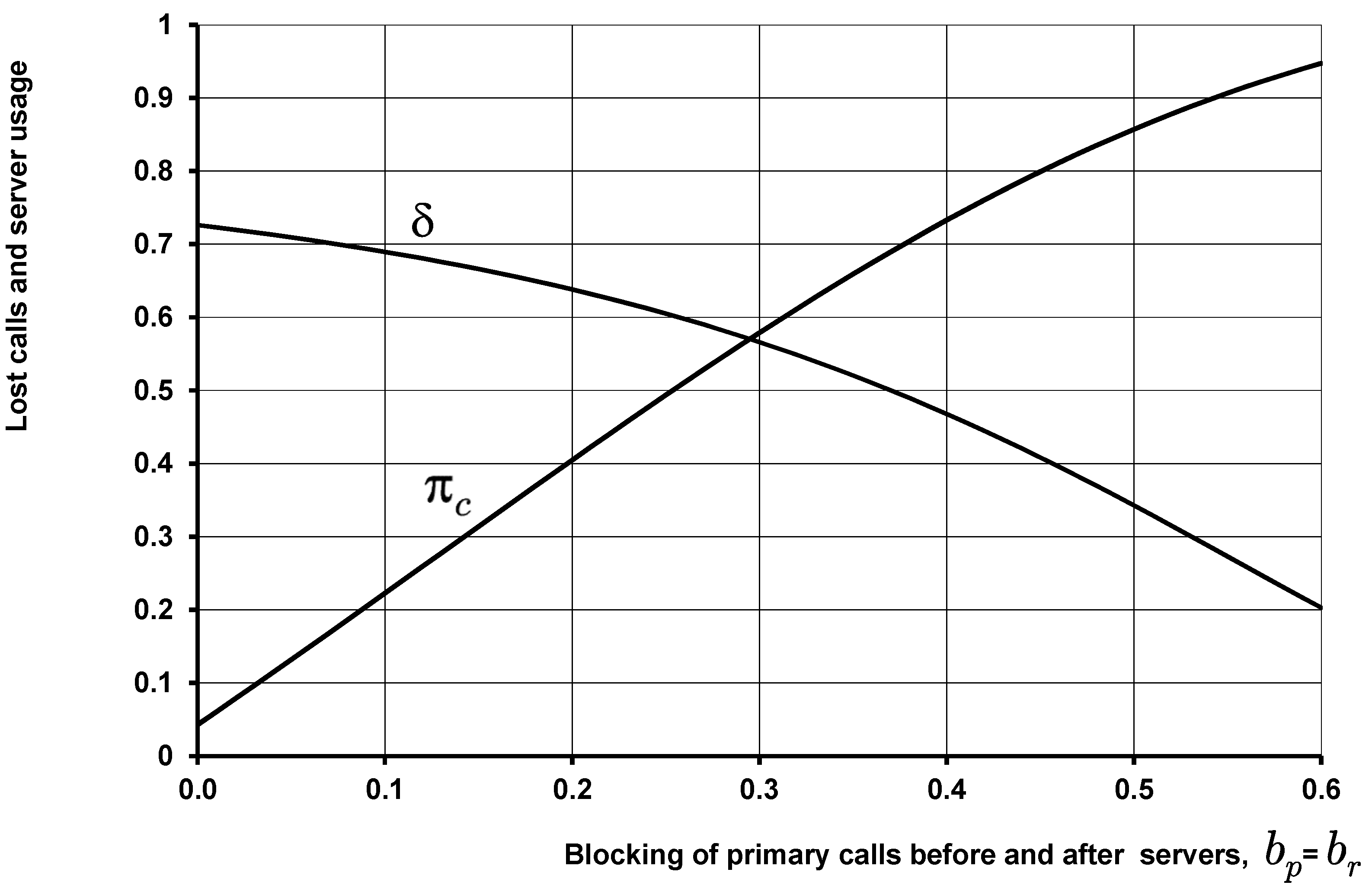
When $b_p=b_r=0$ the blocking before servers does not affect the model performance measurements and ${\pi }_c$, $\delta$ have acceptable for practical implementation levels ${\pi }_c=0.0429$, $\delta =0.7261$. With the increasing of $b_p$ and $b_r$ the ratio of lost calls strongly increases. In contrast, the mean value of one server usage decreases. The presented numerical results show the negative aspects of call losses before servers on values of main performance measures. The situation continues to deteriorate if losses also happen after servers. Additional reasons for call repetition increase the ratio of lost calls and decrease the mean value of server use compared to Figure 3. This result is illustrated in Figure 4 for the same values of input parameters that was used in Figure 3 only with $a_p=b_p$ and $a_r=b_r$.

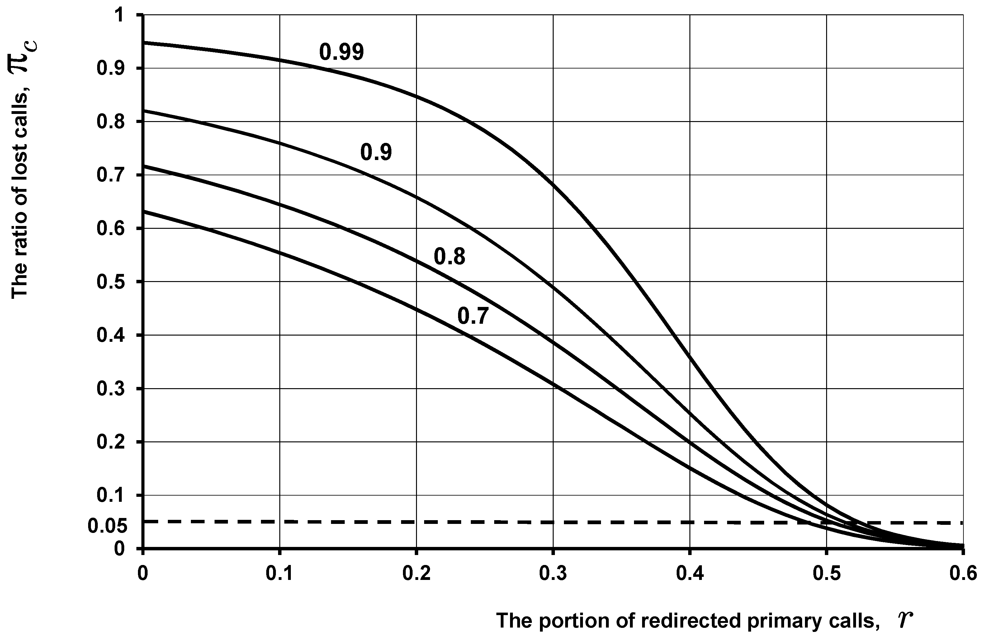
It is well known that emergency services are an object of overload. The overload can be caused by many reasons that are discussed in Section 1. To decrease the negative consequences of overload we can redirect part of the input flow of primary calls to other emergency services with similar functions. The proportion of redirected calls can be found with the help of the constructed model. Let us consider a numerical example. The model’s input parameters are as follows: $\lambda =45$; $v=30$; $\mu =5$; $H_1=H_2$ and takes values $0.7;0.8;0.9;0.99$; $\sigma =0.2$; $b_p=b_r=a_p=a_r=0$.

Figure 5 illustrates the dependence of ${\pi }_c$ on the portion of redirected primary calls r that varies from 0 (no redirection) to $0.6$ for different values of persistence function $H_1=H_2$ that takes values $0.7;0.8;0.9;0.99$. The results of calculations show that by redirecting some part of primary calls we can decrease the value of losses to the prescribed level (here the restriction on ${\pi }_c$ is chosen as ${\pi }_c<0.05$). It is worth mentioning that the required value of redirected primary calls is weakly dependent on the value of probability of repetitions.

6. Discussion

The model of a fully available group of servers with Poisson flow of primary calls and possibility of losses before and after occupying the free server is constructed and analyzed. It is supposed that a call can leave the system because of the aging of transmitted information. All random variables realized in the model have exponential distribution and do not depend on each other. After every loss, a customer with some probability depending on the number of unsuccessful attempt repeats the call. Such models are seen in the modeling of various telecommunication systems such as emergency information services, call and contact centers, access nodes, etc., functioning in an overload situation. The stationary behavior of the system is described by the infinite state Markov process.

A procedure for transforming the model under study has been developed, which makes it possible to exclude the reasons for repeating a call before and after occupation of the server and the possibility of the aging of transmitted information. The procedure consists of four consecutive steps, where each step includes the construction and analysis of an auxiliary model that simplifies the functioning of the generalized model (see Section 4.1, Section 4.2, Section 4.3 and Section 4.4). Thus, the calculation of the model’s performance measures is reduced to the calculation of the characteristics of its particular case with the only reason for the denial of service being the busyness of the servers. The process of calculation is based on constructing and solving the system of state equations. This problem is much easier to solve using an approach based on the concept of a truncated state space. The error caused by truncation is estimated.

The positive features of estimation of the performance measurements based on the concept of a truncated state space lies in the following characteristics:

• The realization of such and approach makes it possible to evaluate characteristics faster, due to the reduction of the used state space and the ability to evaluate characteristics with a predetermined accuracy (see,

  Table A2. Numerical analysis of estimation the performance measures of basic model with retrials based on the truncation of state space.

  $\mathit{\epsilon }$	${\mathit{J}}^{\mathbf{ba}}$	$\frac{|{\mathit{J}}^{\mathbf{ba}}-\mathit{J}|}{\mathit{J}}$	Estimation $\frac{|{\mathit{J}}^{\mathbf{ba}}-\mathit{J}|}{\mathit{J}}$	Effect of Truncation
  ${10}^{-1}$	$1.4166969791$	$1.5\times {10}^{-2}$	$2.4\times {10}^{-2}$	$0.085$
  ${10}^{-2}$	$1.4350225264$	$1.8\times {10}^{-3}$	$2.7\times {10}^{-3}$	$0.113$
  ${10}^{-3}$	$1.4371620706$	$3.0\times {10}^{-4}$	$4.5\times {10}^{-4}$	$0.138$
  ${10}^{-4}$	$1.4375365971$	$4.4\times {10}^{-5}$	$6.2\times {10}^{-5}$	$0.166$
  ${10}^{-5}$	$1.4375920789$	$5.5\times {10}^{-6}$	$7.5\times {10}^{-6}$	$0.196$
  ${10}^{-6}$	$1.4375991299$	$6.0\times {10}^{-7}$	$8.0\times {10}^{-7}$	$0.224$
  ${10}^{-7}$	$1.4375999046$	$5.7\times {10}^{-8}$	$7.4\times {10}^{-8}$	$0.253$
  ${10}^{-8}$	$1.4375999792$	$4.8\times {10}^{-9}$	$6.1\times {10}^{-9}$	$0.282$
  ${10}^{-9}$	$1.4375999848$	$8.6\times {10}^{-10}$	$1.1\times {10}^{-9}$	$0.311$
  ${10}^{-10}$	$1.4375999860$	$5.9\times {10}^{-11}$	$7.4\times {10}^{-11}$	$0.342$

  ). The reduction of counting time, especially noticeable in the analysis of asymptotic cases when intensity of input flow, is increasing (overload) [20].
• A suggested approach allows the avoidance of overflow/underflow problems in computer calculation by taking out of consideration highly unlikely states.
• The values of probabilities are determined from simple recursive relations and do not require matrix inversion. All these properties are of great importance for the implementation of the algorithm in planning tools such as network calculators.

The presented numerical examples illustrate the usage of the model for showing the negative effect of losses before and after occupation of the servers on the model’s performance measures and for the elimination of PSAP overload based on the filtering of the input flow of calls.

The limitations of the obtained results can be summed up as follows:

• The usage of exponential distribution with the same parameter for modeling the service time for all types of incoming requests. This property is necessary for the estimation of the error caused by truncation of the used state space. It does not mean that without this specific characteristic of the model we are not able to implement truncation concept, but in such scenarios finding errors is quite difficult. In most cases it can be done only empirically [20].
• The absence of waiting room for blocked requests. Because of this property, we are not able to estimate the distribution function of waiting time and mean value of waiting.
• The usage of Poisson assumption as a model for primary requests. It should be noted that the Poisson model is used only for constructing the flow of primary calls. The total flow of requests for servicing includes repeated calls and does not follow the Poisson model. By doing this, we are reconstructing the input flow closer to reality, especially when service system is functioning in overload conditions. Retrials are forming a backlog that reflects the quality of request servicing that has been observed in the past. Nevertheless, the acceptability of using Poisson assumption for primary incoming requests needs additional study.

Directions for further research are formulated by taking into consideration above given limitations:

• Find the error of performance measurement estimation caused by the truncation in the general case when service times depend on the type of a call and has exponential distribution with different mean values.
• Generalize the model considered in the paper by taking into account the possibility of waiting and construct an effective algorithm of performance measurement estimation including the mean waiting time and waiting time distribution. Another direction of generalization considers the dependance of probability of call repetition on the type of refusal.
• Study the acceptability of using Poisson assumption for primary requests.

References

1. The European Emergency Number Association Website. Overload of Calls. Available online: https://eena.org/document/overload-of-calls/ (accessed on 28 September 2021).
2. Stepanov, S.N.; Stepanov, M.S.; Shishkin, M.O. Performance Measures of Emergency Services in Case of Overload. In Lecture Notes in Computer Science (LNCS); Vishnevskiy, V., Samouylov, K., Dmitry, V., Kozyrev, D., Eds.; Springer: Cham, Switzerland, 2020; Volume 12563, pp. 436–449. [Google Scholar]
3. Koole, G.M. A Deep Dive into Call Center Workforce Management; MG Books: Amsterdam, The Netherlands, 2020. [Google Scholar]
4. Aksin, O.Z.; Armony, M.; Mehrotra, V. The modern call-center: A multidisciplinary perspective on operations management research. Prod. Oper. Manag. 2007, 16, 665–688. [Google Scholar] [CrossRef] [Green Version]
5. Gans, N.; Koole, G.M.; Mandelbaum, A. Telephone call centers: Tutorial, review, and research prospects. Manuf. Serv. Oper. Manag. 2003, 5, 79–141. [Google Scholar] [CrossRef] [Green Version]
6. Koole, G.; Li, S. A practice-oriented overview of call center workforce planning. arXiv 2021, arXiv:2101.10122. [Google Scholar]
7. Kim, S.; Whitt, W. Are call center and hospital arrivals well modeled by nonhomogeneous poisson processes? Manuf. Serv. Oper. Manag. 2014, 16, 464–480. [Google Scholar] [CrossRef] [Green Version]
8. Green, L.; Kolesar, P. The pointwise stationary approximation for queues with nonstationary arrivals. Manag. Sci. 1991, 37, 84–97. [Google Scholar] [CrossRef] [Green Version]
9. Mandelbaum, A.; Zeltyn, S. Staffing many-server queues with impatient customers: Constraint satisfaction in call centers. Oper. Res. 2009, 57, 1189–1205. [Google Scholar] [CrossRef] [Green Version]
10. Koole, G.M.; Jouini, O.; Roubos, A. Performance indicators for call centers with impatience. IIE Trans. 2013, 45, 341–354. [Google Scholar]
11. Stolletz, R.; Helber, S. Performance Analysis of an Inbound Call Center with Skills-Based Routing: A Priority Queueing System with Two Classes of Impatient Customers and Heterogeneous Agents. OR Spectrum. 2004, 26, 331–352. [Google Scholar] [CrossRef]
12. Stolletz, R. Approximation of the non-stationary M(t)/M(t)/c(t)-queue using stationary queueing models. Eur. J. Oper. Res. 2008, 190, 478–493. [Google Scholar] [CrossRef]
13. Ding, S.; Koole, G.; van der Mei, R.D. On the estimation of the true demand in call centers with redials and reconnects. Eur. J. Oper. Res. 2015, 246, 250–262. [Google Scholar] [CrossRef] [Green Version]
14. Artalejo, R. Accessible bibliography on retrial queues. Math. Comput. Model. 1999, 30, 1–6. [Google Scholar] [CrossRef]
15. Artalejo, J.R. Accessible bibliography on retrial queues: Progress in 2000–2009. Math. Comput. Model. 2010, 51, 1071–1081. [Google Scholar] [CrossRef]
16. Falin, G.I.; Templeton, J.G.C. Retrial Queues; Chapman and Hall: London, UK, 1997. [Google Scholar]
17. Artalejo, R.; Gomez-Corral, A. Retrial Queueing Systems: A Computational Approach; Springer: Berlin, Germany, 2008. [Google Scholar]
18. Stepanov, S.N.; Stepanov, M.S. Algorithms for Estimating Throughput Characteristics in a Generalized Call Center Model. Autom. Remote Control. 2016, 77, 1195–1207. [Google Scholar] [CrossRef]
19. Stepanov, S.N.; Shishkin, M.O.; Stepanov, M.S.; Zhurko, H.M. The construction and analysis of call-center model in overload traffic condition. T-Comm 2020, 14, 42–50. [Google Scholar] [CrossRef]
20. Stepanov, S.N. Markov models with retrials: The calculation of stationary performance measures based on the concept of truncation. Math. Comput. Model. 1999, 30, 207–228. [Google Scholar] [CrossRef]
21. Kim, C.S.; Klimenok, V.I.; Dudin, A.N. Priority tandem queueing system with retrials and reservation of channels as a model of call center. Comput. Ind. Eng. 2016, 96, 61–71. [Google Scholar] [CrossRef]
22. Dudin, S.; Dudina, O. Retrial multi-server queuing system with PHF service time distribution as a model of a channel with unreliable transmission of information. Appl. Math. Model. 2019, 65, 676–695. [Google Scholar] [CrossRef]
23. Anisimov, V.; Artalejo, J. Approximation of multiserver retrial queues by means of generalized truncated models. TOP Off. J. Span. Soc. Stat. Oper. Res. 2002, 10, 51–66. [Google Scholar] [CrossRef]
24. Stepanov, S.N. Generalized model with retrials in case of extreme load. Queueing Syst. 1998, 27, 131–151. [Google Scholar] [CrossRef]
25. Deul, N. Stationary conditions for multi-server queueing systems with repeated calls. J. Inf. Process. Cybern. 1980, 16, 607–613. [Google Scholar]
26. Ionin, G.L.; Sedol, I.I. Telephone systems with repeated calls. In Proceedings of the 6th International Teletraffic Congress, Munich, Germany, 9–15 September 1970; pp. 435.1–435.5. [Google Scholar]
27. Kornyshev, Y.N. A single-line system with repeated orders and preliminary servicing. Eng. Cybern. 1977, 15, 63–68. [Google Scholar]
Figure 1. Bottlenecks in the emergency service chain [1].
Mathematics 09 02811 g001
Figure 2. Functional model of the generalized system with blocked call retrials.
Mathematics 09 02811 g002
Figure 3. Dependence of π c and δ on b p and b r .
Mathematics 09 02811 g003
Figure 4. Dependence of π c and δ on b p , b r , a p and a r .
Mathematics 09 02811 g004
Figure 5. Dependence of π c on the portion of redirected primary calls r for different values of H 1 = H 2 .
Mathematics 09 02811 g005
Publisher’s Note: MDPI stays neutral with regard to jurisdictional claims in published maps and institutional affiliations.