Multivariate Decomposition of Acoustic Signals in Dispersive Channels

Abstract

We present a signal decomposition procedure, which separates modes into individual components while preserving their integrity, in effort to tackle the challenges related to the characterization of modes in an acoustic dispersive environment. With this approach, each mode can be analyzed and processed individually, which carries opportunities for new insights into their characterization possibilities. The proposed methodology is based on the eigenanalysis of the autocorrelation matrix of the analyzed signal. When eigenvectors of this matrix are properly linearly combined, each signal component can be separately reconstructed. A proper linear combination is determined based on the minimization of concentration measures calculated exploiting time-frequency representations. In this paper, we engage a steepest-descent-like algorithm for the minimization process. Numerical results support the theory and indicate the applicability of the proposed methodology in the decomposition of acoustic signals in dispersive channels.

1. Introduction

Signals with time-varying spectral content, known as non-stationary signals, are analyzed using time-frequency signal (TF) signal analysis [1,2,3,4,5,6,7,8,9,10,11,12,13,14,15,16,17]. Some commonly used TF representations include short-time Fourier transform (STFT) [1,3], pseudo-Wigner distribution (WD) [1,9,12], and S-method (SM) [3]. Time-scale, multi-resolution analysis using the wavelet transform is an additional approach to characterize non-stationary signal behavior [4]. Various representations are primarily applied in the instantaneous frequency (IF) estimation and related applications [8,9,10,11,12,13,14,15], since they concentrate the energy of a signal component at and around the respective instantaneous frequency. Concentration measures provide a quantitative description of the signal concentration in the given representation domain [18], and can be used to assess the area of the time-frequency plane covered by a signal component.

In order to characterize multicomponent signals, it is quite common to perform signal decomposition, which assumes that each individual component is extracted for separate analysis, such as for the IF estimation. Decomposition techniques for multicomponent signals are quite efficient if components do not overlap in the time-frequency plane [19,20,21,22,23,24,25,26]. The method originally presented in [26] can be used to completely extract each component by using an intrinsic relation between the PWD and the SM. In the analysis of multicomponent signals, it is, however, common that various components partially overlap in the time-frequency plane, making the decomposition process particularly challenging [19,20,21,22,23,24,25,26]. In this rather unfavorable scenario, overlapped components partially share the same domains of supports, and existing decomposition techniques provide only partial results in the univariate case, limited to very narrow signal classes. For example, linear frequency modulated signals are decomposed using the chirplet transform, Radon transform, or similar techniques [20,25], whereas sinusoidally modulated signals are separated using the inverse Radon transform [27]. However, these techniques cannot perform the decomposition when components have a general, non-stationary form.

In the multivariate (multichannel) framework, it is assumed that the signals are acquired using multiple sensors, [28,29,30,31,32,33,34,35,36,37,38,39,40,41,42,43,44]. The sensors modify component amplitudes and phases. However, the interdependence of values from various channels can be utilized in the signal decomposition. This concept has also been exploited in the empirical mode decomposition (EMD) [39,40,41,42,43]. It was previously shown that WD-based decomposition is possible if signals are available in the multivariate form [28,29,30]. Moreover, the decomposition can be performed by directly engaging the eigenanalysis of the auto-correlation matrix, calculated for signals in the multivariate form [31,32,33,34]. It should also be noted that the problem of multicomponent signal decomposition has some similarities with the blind source separation [45,46,47,48]. However, the basic difference is in the aim to extract each signal component in the decomposition framework, whereas in the blind source separation, the aim is to separate signal sources (although one source may generate several components). The mixing scheme from the blind source separation framework is used in a recently proposed mode decomposition approach [49]. Another line of the decomposition-related research includes mode decomposition techniques, which could be used for separation of modal responses and identification of progressive changes in modal parameters [50].

Overlapped components pose a challenge in various applications, such as in biomedical signal processing [44,51,52], radar signal processing [53], and processing of lamb waves [54]. Popular approaches, such as the EMD and multivariate EMD (MEMD), [39,40,41,42,43] cannot respond to the challenges posed by components overlapped in the time-frequency plane and do not provide acceptable decomposition results in this particular case [28]. Additionally, the applicability of these methods is highly influenced by amplitude variations of the signal components. In this paper, we present a framework for the decomposition of acoustic dispersive environment signals into individual modes based on the multivariate decomposition of multicomponent non-stationary signals. Even when simple signal forms are transmitted, acoustic signals in dispersive channels appear in the multicomponent form, with either very close or partially overlapped components. Being reflected from the underwater surfaces and objects, each individual component carries information about the underwater environment. That information is inaccessible while the signal is in its multicomponent form. This makes analyzing acoustic signals (mainly their localization and characterization) a challenging problem for research [55,56,57,58,59,60]. The presented decomposition approach enables complete separation of components and their individual characterization (e.g., IF estimation, based on which knowledge regarding the underwater environment can be acquired).

We aim at solving this notoriously difficult practical problem by exploiting the interdependencies of multiply acquired signals: such signals can be considered as multivariate and are subject to slight phase changes across various channels, occurring due to different sensing positions and due to various physical phenomena, such as water ripples, uneven seabed, and changes in the seabed substrate. As each eigenvector of the autocorrelation matrix of the input signal represents a linear combination of the signal components [31,33], slight phase changes across the various channels are actually favorable for forming an undetermined set of linearly independent equations relating the eigenvectors and the components. Moreover, we have previously shown that each component is a linear combination of several eigenvectors corresponding to the largest eigenvalues, with unknown weights [31] (the number of these eigenvalues is equal to the number of signal components). Among infinitely many possible combinations of eigenvectors, the aim is to find the weights producing the most concentrated combination, as each individual signal component (mode) is more concentrated than any linear combination of components, as discussed in detail in [31]. Therefore, we engage concentration measures [18] to set the optimization criterion and perform the minimization in the space of the weights of linear combinations of eigenvectors.

We revisit our previous research from [28,31,33], and the main contributions are two-fold. The decomposition principles of the auto-correlation matrix [31,33] are reconsidered. Instead of exploiting direct search [31] or a genetic algorithm [33], we show that the minimization of concentration measure in the space of complex-valued coefficients acting as weights of eigenvectors, which are linearly combined to form the components, can be performed using a steepest-descent-based methodology, originally used in the decomposition from [28]. The second contribution is the consideration of a practical application of the decomposition methodology.

The paper is organized as follows. After the Introduction, we present the basic theory behind the considered acoustic dispersive environment in Section 2. Section 3 presents the principles of multivariate signal decomposition of dispersive acoustic signals. The decomposition algorithm is summarized in Section 4. The theory is verified on numerical examples and additionally discussed in Section 5. Whereas the paper ends with concluding remarks.

2. Dispersive Channels and Shallow Water Theory

Our primary goal is the decomposition of signals transmitted through dispersive channels. Decomposition assumes the separation of signal components while preserving the integrity of each component. Signals transmitted through dispersive channels are multicomponent and non-stationary, even in cases when emitted signals have a simple form. This makes the challenging problem of decomposition, localization, and characterization of such signals a fairly studied topic [55,56,57,58,59,60,61,62,63,64,65,66,67]. The decomposition can be performed using the time-frequency phase-continuity of the signals [55], or using the mode characteristics of the signal [56]. After being transmitted through a dispersive environment, measured signals consist of several components called modes. The non-stationarity of these modes is a consequence of frequency dependent properties of the signal propagation media.

The dispersive acoustic environment is commonly studied within the context of shallow waters, defined by the depth of the sea/ocean, which are less than $D=200$ m [55,57,58,59,60,61,62,63,64,65,66,67]. The speed of signals traveling through water is affected by many factors, such as the salinity, the temperature, or the pressure of the water, but it is usually approximated around 1480–1500 m/s. Note that this speed is larger than the speed of signals traveling through the air, which is estimated at approximately 340–360 m/s. Such setups typically have extremely complex analyses. Moreover, bottom properties and water volume add up to this complexity, as well as noise caused by activities on the water surface and on the coastlines (commonly related to cavitation). Dispersivity of shallow waters occurs due to many reasons, among which are the roughness of the bottom, strength of the waves, and cavity level. Dispersive channels have varying frequency characteristics (phase and spectral content) during the transmission of the signal.

2.1. Normal Mode Solution

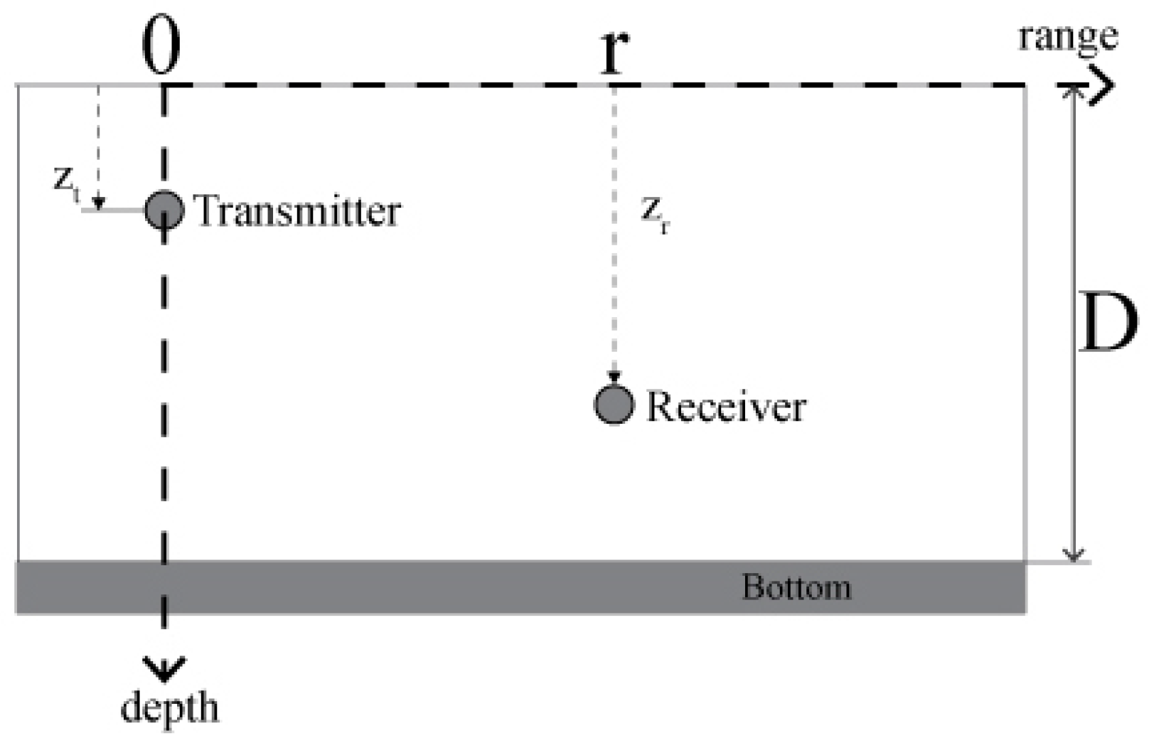
The propagation of sound in a shallow water environment is mathematically represented by the wave equations. Among several methods of deriving the solution of the wave equation, the most commonly used is the normal mode solution, based on solving depth-dependent equations using the method of variable separation. Further analysis will be developed based on the isovelocity waveguide model presented in Figure 1, which characterizes a rigid boundary of the seabed. This further yields to an ideally spread velocity c. Furthermore, channel models assume that the structure of a channel is a waveguide, where multiple normal-modes are received as delayed and scaled versions of the transmitted signal [56,58,59,65]. Our aim is to decompose the received signal by extracting each mode separately. Such extracted modes can be used in further processing, such as IF estimation, characterization, and classification.

More general models assume a more complicated environment, where the boundary of the bottom depends on the nature of the ocean, such as the roughness, depending on the weather conditions and different environments in the ocean itself. These models take into account the scattering of the transmitted signal as well. Our future work will be oriented towards these models as well.

2.2. Problem Formulation—Signal Processing Approach

The practical setup, shown in Figure 1 is further considered. In this setup, it is assumed that the transmitter is located in the water at the depth of $z_t$, whereas the receiver is located at the depth of $z_r$ meters. It is assumed that the wave is transmitted through an isovelocity channel as in [55,56,57,61,62,63,67]. The distance between the transmitter and the receiver is r.

Taking into account the spectrum of the received signal, in the normal-mode case, the transfer function reads

$$\begin{array}{c}H\left(\omega \right)=\sum _{p=1}^{+\infty }{G}_p\left(z_t\right)G_p\left(z_r\right)\frac{exp\left(j{k}_r(p,\omega )r\right)}{\sqrt{k_r(p,\omega )r}}=\sum _{p=1}^{+\infty }{A}_t(p,\omega )exp\left(j{k}_r(p,\omega )r\right),\end{array}$$

(1)

with $G_p\left(z_t\right)$ and $G_p\left(z_r\right)$ being the modal functions of the p-th mode corresponding to the transmitter and the receiver [55,56,65], with the attenuation rate is $A_t(p,\omega )=A(p,\omega )/\sqrt{r}$. Angular frequency is denoted by $\omega$. The modes are dependent on wavenumbers $k_r(p,\omega )$ [55]

$$k_r^2(p,\omega )={\left(\frac{\omega }{c}\right)}^2-{\left((p-0.5)\frac{\pi }{D}\right)}^2.$$

(2)

The multicomponent structure of the transfer function is dependent on the number of modes. The speed of sound propagation underwater is $c=1500$ m/s.

The response to a monochromatic signal

$$s\left(n\right)=exp\left(j{\omega }_{0}n\right)$$

(3)

at the p-th mode can be written as

$$s_p\left(n\right)\approx A_t(p,{\omega }_0)exp(j{\omega }_{0}n-j{k}_r(p,{\omega }_0)r).$$

(4)

The phase velocity of this signal is

$${\nu }_p\left(\omega \right)=\frac{\omega }{k_r(p,\omega )}=\frac{\omega }{\sqrt{{\left(\frac{\omega }{c}\right)}^2-{\left((p-0.5)\frac{\pi }{D}\right)}^2}}.$$

(5)

This is the horizontal velocity of the corresponding phase for the p-th mode. The energy propagation of the signal component is represented by the group velocity

$$u_p\left(\omega \right)=\frac{dr\left(t\right)}{dt}=\frac{d\omega }{d{k}_r(p,\omega )}=\frac{1}{\frac{d{k}_r(p,\omega )}{d\omega }}=\frac{1}{\frac{d}{d\omega }\sqrt{{\left(\frac{\omega }{c}\right)}^2-{\left((p-0.5)\frac{\pi }{D}\right)}^2}}.$$

(6)

The received signal can be represented in the Fourier transform domain as a product of the Fourier transform of the transmitted signal, $S\left(\omega \right)$ and the transfer function $H\left(\omega \right)$ of the channel in the normal-mode form; that is

$$X\left(\omega \right)=S\left(\omega \right)H\left(\omega \right).$$

(7)

In time domain, the received signal, $x\left(n\right)$, is the convolution of the transmitted signal, $s\left(n\right)$ and the impulse response, $h\left(n\right)$, from (1), i.e.,

$$x\left(n\right)=s\left(n\right)\ast h\left(n\right).$$

(8)

In the following sections, we present an efficient methodology for the decomposition of mode functions, which will make the problem of detecting and estimating the received signal parameters straightforward.

3. Multivariate Decomposition

3.1. Multivariate (Multichannel) Signals

Multivariate or multichannel signals are acquired using multiple sensors. It is further assumed that C sensors at the receiving position are used for the acquisition of signal $x_R\left(n\right)$. Here, subscript R is used to denote the fact that the acquired signal is real-valued. All C sensors placed at the depth $z_r$ are part of the receiver. In the range direction, sensor distances from the transmitter are $r+{\delta }_c$, $c=1,2,\cdots ,C$. Deviations ${\delta }_c$, $c=1,2,\cdots ,C$, are small as compared to the distance, r, between the transmitter and receiver locations in Figure 1 in range direction.

Since the measured signal, $x_R\left(n\right)$, is real-valued, its analytic extension

$$x\left(n\right)=x_R\left(n\right)+j\mathcal{H}\left\{x_R\left(n\right)\right\}$$

(9)

is assumed in the further multivariate decomposition setup, where $\mathcal{H}\left\{x_R\left(n\right)\right\}$ is the Hilbert transform of this signal. This analytic form assumes only non-negative frequencies. Each sensor modifies the amplitude and the phase of the acquired signal. Therefore, the channel signals take the form $a_c\left(n\right)exp\left(j{\varphi }_c\left(n\right)\right)={\alpha }_{c}exp\left(j{\phi }_c\right)x\left(n\right)$, for each sensor $c=1,2,\cdots ,C$. When a monocomponent signal $x\left(n\right)=A\left(n\right)exp\left(j\psi \right(n\left)\right)$, is measured at sensor c, this yields

$$a_c\left(n\right)exp\left(j{\varphi }_c\left(n\right)\right)={\alpha }_{c}exp\left(j{\phi }_c\right)x\left(n\right),$$

or $a_c\left(n\right)cos\left({\varphi }_c\left(n\right)\right)$ in the case of a real-valued signal. The corresponding analytic signal, $a_i\left(n\right)exp\left(j{\varphi }_i\left(n\right)\right)=a_i\left(n\right)cos\left({\varphi }_i\left(n\right)\right)+j\mathcal{H}\{a_i\left(n\right)cos\left({\varphi }_i\left(n\right)\right)\}$ is a valid representation of the real amplitude-phase signal $a_c\left(n\right)cos\left({\varphi }_c\left(n\right)\right)$ if the spectrum of $a_i\left(n\right)$ is nonzero only within the frequency range $\left|\omega \right|<B$ and the spectrum of $cos\left({\varphi }_i\left(n\right)\right)$ occupies a non-overlapping (much) higher frequency range [5]. If variations of the amplitude, $a_c\left(n\right)$, are much slower than the phase ${\varphi }_c\left(n\right)$ variations, then this signal is monocomponent [31]. A unified representation of a multichannel (multivariate) signal, acquired using C sensors, assumes the following vector form

$$\mathbf{x}\left(n\right)=\left[\begin{array}{c}{x}^{\left(1\right)}\left(n\right)\\ x^{\left(2\right)}\left(n\right)\\ ⋮\\ x^{\left(C\right)}\left(n\right)\end{array}\right]=\left[\begin{array}{c}{a}_1\left(n\right)e^{j{\varphi }_1\left(n\right)}\\ a_2\left(n\right)e^{j{\varphi }_2\left(n\right)}\\ ⋮\\ a_C\left(n\right)e^{j{\varphi }_C\left(n\right)}\end{array}\right],n=1,2,\cdots ,N.$$

(10)

3.2. Multivariate Multicomponent Signals

When the measured signal consists of a linear combination of P linearly independent components $s_p\left(n\right)=A_p\left(n\right)e^{j{\psi }_p\left(n\right)}$, $p=1,2,\cdots ,P$, then it is commonly referred to as a multicomponent signal

$$x\left(n\right)=\sum _{p=1}^P{s}_p\left(n\right)=\sum _{p=1}^P{A}_p\left(n\right)e^{j{\psi }_p\left(n\right)}.$$

(11)

Component amplitudes, $A_p\left(n\right)$, are characterized by slow-varying dynamics as compared to the variations of the component phases, ${\psi }_p\left(n\right)$. Linear independence of the components assumes that neither component can be represented as a linear combination of other components for any considered time instant n.

Incorporation of multicomponent signal definition (11) into the multichannel form (10), yields

$$\mathbf{x}\left(n\right)=\left[\begin{array}{c}{x}^{\left(1\right)}\left(n\right)\\ x^{\left(2\right)}\left(n\right)\\ ⋮\\ x^{\left(C\right)}\left(n\right)\end{array}\right]=\left[\begin{array}{c}{a}_1\left(n\right)e^{j{\varphi }_1\left(n\right)}\\ a_2\left(n\right)e^{j{\varphi }_2\left(n\right)}\\ ⋮\\ a_C\left(n\right)e^{j{\varphi }_C\left(n\right)}\end{array}\right]=\left[\begin{array}{c}\sum _{p=1}^P{\alpha }_{1p}{s}_p\left(n\right)e^{j{\phi }_{1p}}\\ \sum _{p=1}^P{\alpha }_{2p}{s}_p\left(n\right)e^{j{\phi }_{2p}}\\ ⋮\\ \sum _{p=1}^P{\alpha }_{Cp}{s}_p\left(n\right)e^{j{\phi }_{Cp}}\end{array}\right],n=1,2,\cdots ,N,$$

(12)

or, more briefly,

$$\left[\begin{array}{c}{x}^{\left(1\right)}\left(n\right)\\ x^{\left(2\right)}\left(n\right)\\ ⋮\\ x^{\left(C\right)}\left(n\right)\end{array}\right]=\left[\begin{array}{cccc}{a}_{11}& a_{12}& \cdots & a_{1P}\\ a_{21}& a_{22}& \cdots & a_{2P}\\ ⋮& ⋮& \ddots & ⋮\\ a_{C1}& a_{C2}& \cdots & a_{CP}\end{array}\right]\left[\begin{array}{c}{s}_1\left(n\right)\\ s_2\left(n\right)\\ ⋮\\ s_P\left(n\right)\end{array}\right],$$

(13)

that is

$$\mathbf{x}\left(n\right)=\mathbf{As}\left(n\right),$$

(14)

where the vector of signal components, $\mathbf{s}\left(n\right)$ is, for instant n, given by

$$\mathbf{s}\left(n\right)=\left[\begin{array}{c}{s}_1\left(n\right)\\ s_2\left(n\right)\\ ⋮\\ s_P\left(n\right)\end{array}\right],n=1,2,\cdots ,N.$$

(15)

Matrix $\mathbf{A}$ of size $C\times P$, which relates the signal in the c-th channel, $x^{\left(c\right)}\left(n\right)$ with signal components, $s_p\left(n\right)$, in form of a linear combination

$$x^{\left(c\right)}\left(n\right)=\sum _{p=1}^P{a}_{cp}{s}_p\left(n\right)=\sum _{p=1}^P{\alpha }_{cp}{s}_p\left(n\right)e^{j{\varphi }_{cp}}$$

(16)

has the following form

$$\mathbf{A}=\left[\begin{array}{cccc}{a}_{11}& a_{12}& \cdots & a_{1P}\\ a_{21}& a_{22}& \cdots & a_{2P}\\ ⋮& ⋮& \ddots & ⋮\\ a_{C1}& a_{C2}& \cdots & a_{CP}\end{array}\right],$$

with elements being complex constants $a_{cp}={\alpha }_{cp}{e}^{j{\phi }_{cp}}$, $c=1,2,\cdots ,C$, $p=1,2,\cdots ,P$. These constants linearly relate the channel signals with signal components. Clearly, the maximum number of independent channels $x^{\left(1\right)}\left(n\right)$, $x^{\left(2\right)}\left(n\right),\cdots$, $x^{\left(C\right)}\left(n\right)$ in $\mathbf{x}\left(n\right)$ is

$$M=min\{C,P\},$$

(17)

since $\mathrm{rank}\left\{\mathbf{A}\right\}\le min\{C,P\}$.

The relation between the C measured channel signals, $x^{\left(c\right)}\left(n\right)$, and P components, $x_p\left(n\right)$, can be, taking into consideration all time instants, formed by introducing $C\times N$ matrix ${\mathbf{X}}_{sen}$ with elements being the sensed signal values, and ${\mathbf{X}}_{com}$ comprising the samples of signal components $s_p\left(n\right)$. In that case, the relation is

$$\left[\begin{array}{ccc}{x}^{\left(1\right)}\left(1\right)& \cdots & x^{\left(1\right)}\left(N\right)\\ x^{\left(2\right)}\left(1\right)& \cdots & x^{\left(2\right)}\left(N\right)\\ ⋮& \ddots & ⋮\\ x^{\left(C\right)}\left(1\right)& \cdots & x^{\left(C\right)}\left(N\right)\end{array}\right]=\mathbf{A}\left[\begin{array}{ccc}{s}_1\left(1\right)& \cdots & s_1\left(N\right)\\ s_2\left(1\right)& \cdots & s_2\left(N\right)\\ ⋮& \ddots & ⋮\\ s_P\left(1\right)& \cdots & s_P\left(N\right)\end{array}\right].$$

(18)

or

$${\mathbf{X}}_{sen}=\mathbf{A}{\mathbf{X}}_{com}.$$

(19)

Now we can introduce the autocorrelation matrix $\mathbf{R}$ of the sensed signal, whose eigenvectors will be used in the multivariate decomposition framework:

$$\begin{array}{c}\hfill \mathbf{R}={\mathbf{X}}_{sen}^H{\mathbf{X}}_{sen},\end{array}$$

(20)

where ${(·)}^H$ denotes the Hermitian transpose. Individually, elements of this matrix are products of $\mathbf{x}\left(n_1\right)$ and ${\mathbf{x}}^H\left(n_1\right)$ at given instants $n_1$ and $n_2$:

$$\begin{array}{c}\hfill R(n_1,n_2)={\mathbf{x}}^H\left(n_2\right)\mathbf{x}\left(n_1\right)=\sum _{i=1}^C{x}^{\left(i\right)*}\left(n_2\right)x^{\left(i\right)}\left(n_1\right),\end{array}$$

(21)

where $\mathbf{x}\left(n_1\right)={[x^{\left(1\right)}\left(n_1\right)x^{\left(2\right)}\left(n_1\right)\cdots x^{\left(C\right)}\left(n_1\right)]}^T$ is the column vector of sensed values at a given instant $n_1$. As it will be shown next, the eigenvectors of the autocorrelation matrix, $\mathbf{R}$, corresponding to the largest eigenvalues, consist of linear combinations of signal components. This fact will be used to develop the algorithm for the extraction of those components.

3.3. Eigendecomposition of the Autocorrelation Matrix

It is well-known that any square matrix $\mathbf{R}$, of dimensions $K\times K$, can be subject of eigenvalue decomposition

$$\mathbf{R}=\mathbf{Q}\Lambda {\mathbf{Q}}^H=\sum _{p=1}^K{\lambda }_p{\mathbf{q}}_p{\mathbf{q}}_p^H,$$

(22)

with ${\lambda }_p$ being the eigenvalues and ${\mathbf{q}}_p$ being the corresponding eigenvectors of matrix $\mathbf{R}$. Matrix $\Lambda$ contains eigenvalues ${\lambda }_p$, $p=1,2,\cdots ,K$ on the main diagonal and zeros at other positions. Matrix $\mathbf{Q}=\left[{\mathbf{q}}_1,{\mathbf{q}}_2,\cdots ,{\mathbf{q}}_K\right]$ contains the eigenvectors ${\mathbf{q}}_p$ as its columns. Since $\mathbf{R}$ is symmetric, eigenvectors are orthogonal.

From definition (20) and based on relation ${\mathbf{X}}_{sen}=\mathbf{A}{\mathbf{X}}_{com}$, autocorrelation matrix $\mathbf{R}$ can be rewritten as

$$\mathbf{R}={\mathbf{X}}_{sen}^H{\mathbf{X}}_{sen}={\mathbf{X}}_{com}^H{\mathbf{A}}^H\mathbf{A}{\mathbf{X}}_{com}=\sum _{i=1}^P\sum _{j=1}^P{\overline{a}}_{ij}{\mathbf{s}}_i{\mathbf{s}}_j^H,$$

(23)

where ${\overline{a}}_{ij}$ is used to denote elements of matrix ${\mathbf{A}}^H\mathbf{A}$ and ${\mathbf{s}}_i={\left[s_i\left(1\right),s_i\left(2\right),\cdots s_i\left(N\right)\right]}^H$. Elements of matrix $\mathbf{R}$ are

$$R(n_1,n_2)=\sum _{i=1}^P\sum _{j=1}^P{\overline{a}}_{ij}{s}_i\left(n_1\right)s_j^{*}\left(n_2\right)=\left[\begin{array}{c}{s}_1^{*}\left(n_2\right),s_2^{*}\left(n_2\right),\cdots ,s_P^{*}\left(n_2\right)\end{array}\right]{\mathbf{A}}^{\mathbf{H}}\mathbf{A}\left[\begin{array}{c}{s}_1\left(n_1\right)\\ s_2\left(n_1\right)\\ ⋮\\ s_P\left(n_1\right)\end{array}\right].$$

(24)

Based on the decomposition of matrix $\mathbf{R}$ on its eigenvalues and eigenvectors, we further have

$$\mathbf{R}=\sum _{p=1}^M{\lambda }_p{\mathbf{q}}_p{\mathbf{q}}_p^H=\sum _{i=1}^P\sum _{j=1}^P{\overline{a}}_{ij}{\mathbf{s}}_i{\mathbf{s}}_j^H,$$

(25)

with $M=min\{C,P\}$. It will be further assumed that the number of sensors, C is such that $C\ge P$. In that case, there are $M=P$ eigenvectors in (25). Two general cases can be further discussed:

• Non-overlapped components. Note that the case when no components ${\mathbf{s}}_i$ and ${\mathbf{s}}_j$ overlap in the time-frequency plane implies that these components are orthogonal. In that case, the right side of (25) becomes:

  $$\mathbf{R}=\sum _{i=1}^P{\mathbf{s}}_i{\mathbf{s}}_i^H\sum _{j=1}^P{\overline{a}}_{ij}={\kappa }_p\sum _{p=1}^P{\mathbf{s}}_p{\mathbf{s}}_p^H=\sum _{p=1}^P{\lambda }_p{\mathbf{q}}_p{\mathbf{q}}_p^H$$

  (26)

  where ${\kappa }_p={\sum }_{j=1}^P{\overline{a}}_{ij}$. The considered case of non-overlapped (orthogonal) components further implies that

  $${\kappa }_p{\mathbf{s}}_p={\lambda }_p{\mathbf{q}}_p,p=1,2,\cdots ,P.$$

  (27)
• Partially overlapped components. Based on (25), since the partially overlapped components are non-orthogonal; that is, such components are linearly dependent, eigenvectors can be expressed as linear combinations of such components

  $$\begin{array}{cc}\hfill {\mathbf{q}}_1& ={\xi }_{11}{\mathbf{s}}_1+{\xi }_{21}{\mathbf{s}}_2+\cdots +{\xi }_{P1}{\mathbf{s}}_P\hfill \\ \hfill {\mathbf{q}}_2& ={\xi }_{12}{\mathbf{s}}_1+{\xi }_{22}{\mathbf{s}}_2+\cdots +{\xi }_{P2}{\mathbf{s}}_P\hfill \\ & ⋮\\ \hfill {\mathbf{q}}_M& ={\xi }_{1M}{\mathbf{s}}_1+{\xi }_{2M}{\mathbf{s}}_2+\cdots +{\xi }_{PM}{\mathbf{s}}_P,\hfill \end{array}$$

  (28)

  with $M=min\{C,P\}$, i.e., for assumed $C\ge P$, $M=P$.

3.4. Components as the Most Concentrated Linear Combinations of Eigenvectors

Based on (28) and for assumed $M=P$, each signal component, ${\mathbf{s}}_p$ can be expressed as a linear combination of eigenvectors ${\mathbf{q}}_p$ of matrix $\mathbf{R}$, $p=1,2,\cdots ,P$; that is

$$\begin{array}{c}{\mathbf{s}}_p={\gamma }_{1p}{\mathbf{q}}_1+{\gamma }_{2p}{\mathbf{q}}_2+\cdots +{\gamma }_{Pp}{\mathbf{q}}_P,\end{array}$$

(29)

where ${\gamma }_{ip}$, $i=1,2,\cdots P$, $p=1,2,\cdots P$ are unknown coefficients. Obviously, there are $M=P$ linear equations for P components, with $P^2$ unknown weights. Among infinitely many solutions of this undetermined system of equations, we aim at finding those combinations that produce signal components. Moreover, since components are partially overlapped, in the case when one component is detected, its contribution should be removed from all equations (linear combinations of eigenvectors) in order to avoid that it is detected again.

Obviously, for the detection of linear combinations of eigenvectors, which represent signal components, a proper detection criterion shall be established. Since non-stationary signals can be suitably represented using time-frequency representations, and signal components tend to be concentrated along their instantaneous frequencies, our criterion will be based on time-frequency representations.

Time-frequency signal analysis provides a mathematical framework for a joint representation of signals in time and frequency domains. If $w\left(m\right)$ denotes a real-valued, symmetric window function of length $N_w$, then signal $s_p\left(n\right)$ can be represented using the STFT

$$STF{T}_p(n,k)=\sum _{m=0}^{N_w-1}w\left(m\right)s_p(n+m)e^{-j2\pi mk/N_w},$$

(30)

which renders the frequency content of the portion of signal around the each considered instant n, localized by the window function $w\left(n\right)$.

To determine the level of the signal concentration in the time-frequency domain, we can exploit concentration measures. Among various approaches, inspired by the recent compressed sensing paradigm, measures based on the ${\ell }_{\rho }$ norm of the STFT have been used lately [18]

$$\begin{array}{c}\mathcal{M}\left\{STF{T}_p(n,k)\right\}={\parallel STFT(n,k)\parallel }_{\rho }^{\rho }\\ =\sum _n\sum _k{\left|STFT(n,k)\right|}^{\rho }=\sum _n\sum _{k}SPE{C}^{\rho /2}(n,k),\end{array}$$

(31)

where $SPEC(n,k)={\left|STFT(n,k)\right|}^2$ represents the commonly used spectrogram, whereas $0\le \rho \le 1$. For $\rho =1$, the ${\ell }_1$-norm is obtained.

We consider P components, $s_p\left(n\right),p=1,2,\cdots ,P$. Each of these components has finite support in the time-frequency domain, ${\mathbb{P}}_p$, with areas of support ${\Pi }_p$, $p=1,2,\cdots ,P$. Supports of partially overlapped components are also partially overlapped. Furthermore, we will make a realistic assumption that there are no components that overlap completely. Assume that ${\Pi }_1\le {\Pi }_1\le \cdots \le {\Pi }_P$.

Consider further the concentration measure $\mathcal{M}\left\{STF{T}_p(n,k)\right\}$ of

$$\mathbf{y}={\eta }_1{\mathbf{q}}_1+{\eta }_2{\mathbf{q}}_2+\cdots +{\eta }_P{\mathbf{q}}_{P,}$$

(32)

for $p=0$. If all components are present in this linear combination, then the concentration measure ${\parallel STFT(n,k)\parallel }_0$, obtained for $p=0$ in (31), will be equal to the area of ${\mathbb{P}}_1\cup {\mathbb{P}}_2\cup \cdots {\mathbb{P}}_P$.

If the coefficients ${\eta }_p$, $p=1,2,\cdots ,P$ are varied, then the minimum value of the ${\ell }_0$-norm based concentration measure is achieved for coefficients ${\eta }_1={\gamma }_{11},{\eta }_2={\gamma }_{21},\cdots ,{\eta }_P={\gamma }_{P1}$ corresponding to the most concentrated signal component $s_1\left(n\right)$, with the smallest area of support, ${\Pi }_1$, since we have assumed, without the loss of generality, that ${\Pi }_1\le {\Pi }_1\le \cdots \le {\Pi }_P$ holds. Note that, due to the calculation and sensitivity issues related with the ${\ell }_0$-norm, within the compressive sensing area, ${\ell }_1$-norm is widely used as its alternative, since under reasonable and realistic conditions, it produces the same results [31]. Therefore, it can be considered that the areas of the domains of support in this context can be measured using the ${\ell }_1$-norm.

The problem of extracting the first component, based on eigenvectors of the autocorrelation matrix of the input signal, can be formulated as follows

$$\begin{array}{c}\hfill [{\beta }_{11},{\beta }_{21},\cdots ,{\beta }_{P1}]=arg\underset{{\eta }_1,\cdots ,{\eta }_P}{min}{\parallel STFT(n,k)\parallel }_1.\end{array}$$

(33)

The resulting coefficients produce the first component (candidate)

$${\overline{\mathbf{s}}}_1={\beta }_{11}{\mathbf{q}}_1+{\beta }_{21}{\mathbf{q}}_2+\cdots +{\beta }_P{\mathbf{q}}_{P1.}$$

(34)

Note that if ${\beta }_{11}={\gamma }_{11},{\beta }_{21}={\gamma }_{21},\cdots {\beta }_{P1}={\gamma }_{P1}$ holds, then the component is exact; that is, ${\overline{\mathbf{s}}}_1={\mathbf{s}}_1$ holds. In the case when the number of signal components is larger than two, the concentration measure in (33) can have several local minima in the space of unknown coefficients ${\eta }_1,{\eta }_2,\cdots ,{\eta }_P$, corresponding not only to individual components but also to linear combinations of two, three or more components. Depending on the minimization procedure, it can happen that the algorithm finds this local minimum; that is, a set of coefficients producing a combination of components instead of an individual component. In that case, we have not extracted successfully a component since ${\overline{\mathbf{s}}}_1\ne {\mathbf{s}}_1$ in (34), but as it will be discussed next, this issue does not affect the final result, as the decomposition procedure will continue with this local minimum eliminated.

3.5. Extraction of Detected Component and Further Decomposition

Upon detection of the first local minimum, being a signal component or a linear combination of several components, ${\overline{\mathbf{s}}}_1$, first eigenvector, ${\mathbf{q}}_1$ should be replaced by ${\overline{\mathbf{s}}}_1$ in the linear combination

$$\mathbf{y}={\eta }_1{\mathbf{q}}_1+{\eta }_2{\mathbf{q}}_2+\cdots +{\eta }_P{\mathbf{q}}_{P,}$$

(35)

i.e., ${\mathbf{q}}_1={\overline{\mathbf{s}}}_{\mathbf{1}}$ is further used as the first eigenvector. However, since (28) holds, the contribution of this detected component (or linear combination of components) is still present in remaining eigenvectors ${\mathbf{q}}_p,p=2,3,\cdots ,P$ and shall be removed from these eigenvectors as well. To this aim, we utilize the signal deflation theory [31], and remove the projections of this component from remaining eigenvectors using

$${\mathbf{q}}_p=\frac{{\mathbf{q}}_p-{\mathbf{q}}_1^H{\mathbf{q}}_p{\mathbf{q}}_1}{\sqrt{1-|{\mathbf{q}}_1^H{\mathbf{q}}_p{|}^2}}.$$

(36)

This ensures that ${\overline{\mathbf{s}}}_1$ is not repeatedly detected afterward. If ${\overline{\mathbf{s}}}_1={\mathbf{s}}_1$, then the first component is found and extracted, whereas its projection on other eigenvectors is removed.

The described procedure is then repeated iteratively, with linear combination $\mathbf{y}={\eta }_1{\mathbf{q}}_1+{\eta }_2{\mathbf{q}}_2+\cdots +{\eta }_P{\mathbf{q}}_P$ with first eigenvector ${\mathbf{q}}_1={\overline{\mathbf{s}}}_1$ and eigenvectors ${\mathbf{q}}_p,p=1,2,\cdots ,P$, modified according to (36). Upon detecting the second component (or linear combination of a small number of components), ${\overline{\mathbf{s}}}_2$, the second eigenvector is replaced, ${\mathbf{q}}_1={\overline{\mathbf{s}}}_2$, whereas its projections from remaining eigenvectors is removed using

$${\mathbf{q}}_p=\frac{{\mathbf{q}}_p-{\mathbf{q}}_2^H{\mathbf{q}}_p{\mathbf{q}}_2}{\sqrt{1-|{\mathbf{q}}_2^H{\mathbf{q}}_p{|}^2}}.$$

(37)

The process repeats until all components are detected and extracted. These principles are incorporated into the decomposition algorithm presented in the next section.

4. The Decomposition Algorithm and Concentration Measure Minimization

4.1. Decomposition Algorithm

The decomposition procedure can be summarized with the following steps:

• For given multivariate signal

  $$\mathbf{x}\left(n\right)=\left[\begin{array}{c}{x}^{\left(1\right)}\left(n\right)\\ x^{\left(2\right)}\left(n\right)\\ ⋮\\ x^{\left(C\right)}\left(n\right)\end{array}\right]$$

  calculate the input autocorrelation matrix

  $$\mathbf{R}={\mathbf{X}}_{sen}^H{\mathbf{X}}_{sen}$$

  (38)

  where    

  $${\mathbf{X}}_{sen}=\left[\begin{array}{ccc}{x}^{\left(1\right)}\left(1\right)& \cdots & x^{\left(1\right)}\left(N\right)\\ x^{\left(2\right)}\left(1\right)& \cdots & x^{\left(2\right)}\left(N\right)\\ ⋮& \ddots & ⋮\\ x^{\left(C\right)}\left(1\right)& \cdots & x^{\left(C\right)}\left(N\right)\end{array}\right].$$

  (39)
• Find eigenvectors ${\mathbf{q}}_p$ and eigenvalues ${\lambda }_p$, $p=1,2,\cdots ,P$ of matrix $\mathbf{R}$.
  It should be noted that the number of components, P, can be estimated based on the eigenvalues of matrix $\mathbf{R}$. Namely, as discussed in [31], P largest eigenvalues of matrix R correspond to signal components. These eigenvalues are larger than the remaining $N-P$ eigenvalues. This property holds even in the presence of a high-level noise: a threshold for separation of eigenvalues corresponding to signal components can be easily determined based on the input noise variance [28].
• Initialize variable $N_u=0$ and variable $k=0$. Variable $N_u$ will store the number of updates of eigenvectors ${\mathbf{q}}_p$, $p\ne i$ when projection of detected component (candidate) is removed from eigenvectors ${\mathbf{q}}_p$, $p\ne i$. Variable k represents the index of the detected components.
• For $i=1,2,\cdots ,P$, repeat the following steps:

  (a)

  Solve minimization problem

  $$\underset{{\beta }_{1k},\dots ,{\beta }_{Pk}}{min}{∥STFT\left\{\frac{1}{C}\sum _{p=1}^P{\beta }_{pk}{\mathbf{q}}_p\right\}∥}_1\mathrm{subject}\mathrm{to}{\beta }_{ik}=1$$

  where $STFT\{·\}$ is the STFT operator. Signal $\mathbf{y}=\frac{1}{C}{\sum }_{p=1}^P{\beta }_{pk}{\mathbf{q}}_p$ is scaled with

  $$C=\sqrt{{∥{\sum }_{p=1}^P{\beta }_{pk}{\mathbf{q}}_p∥}_2}$$

  in order to normalize energy of the combined signal to 1. Coefficients ${\beta }_{1k},{\beta }_{2k},\dots ,{\beta }_{Pk}$ are obtained as a result of the minimization.

  (b)

  Increment component index $k\leftarrow k+1$

  (c)

  If for any $p\ne i$, ${\beta }_{pk}\ne 0$ holds, then

  • Increment variable $N_u\leftarrow N_u+1$
  • Upon replacing the i-th eigenvector by the detected component,

    $${\mathbf{q}}_i=\frac{1}{C}\sum _{p=1}^P{\beta }_{pk}{\mathbf{q}}_p$$

    (40)

    remove projections of detected component (candidate) from remaining eigenvectors. For $l=i+1,i+2,\cdots ,P$ repeat:
    • $b={\mathbf{q}}_i^H{\mathbf{q}}_l$
    • ${\mathbf{q}}_l=\frac{1}{\sqrt{1-{\left|b\right|}^2}}({\mathbf{q}}_l-b{\mathbf{q}}_i)$

• If $N_u>0$, return to Step 3.

Finally, as a result, we obtain the number of components, P, and the set of extracted components, ${\mathbf{q}}_1,{\mathbf{q}}_1,\cdots ,{\mathbf{q}}_P$.

It should be noted that checking whether $N_u>0$ holds in Step 5 is crucial for removing possibly detected local minima of concentration measure not corresponding to individual components, but to a linear combination of several components. Namely, if this situation happens, upon applying signal deflation by removing projection of the linear combination of components from other eigenvectors, a linear dependence among eigenvectors will still remain, and it will not allow $N_u$ to fall to zero. This returns the algorithm to Step 3, and the procedure for the component detection repeats, but with the local minimum removed from the concentration measure since all the eigenvectors are already updated in the previous cycle. Note that the component index k is reset to zero in this case.

Moreover, it should be emphasized that, while the presented procedure produces P eigenvectors, which is exactly equal to the given number of components, this number is not always a priori known. In practical applications, it can be determined based on eigenvalues of matrix $\mathbf{R}$. As it will be illustrated in numerical examples, the largest eigenvalues correspond to signal components [28,31]. The remaining eigenvalues correspond to the noise. Therefore, a simple threshold can be used to calculate the exact number of signal components. Namely, we simply count the number of eigenvalues larger than a predefined threshold T, being a small positive constant. In the presence of the noise, threshold T should be at least equal to the noise variance. The larger the noise, the larger are the eigenvalues corresponding to the noise (thus, larger should the threshold T be). Of course, the procedure works without the exact information about the number of components: for $p>P$, eigenvectors ${\mathbf{q}}_p$ contain only the noise after the decomposition is finished.

4.2. Concentration Measure Minimization

The concentration measure minimization is performed in the steepest descent manner, as presented in Algorithm 1. The coefficient ${\beta }_{pk}=1$ is fixed for $p=i$, whereas the values of other coefficients are varied for $\pm \Delta$. Note that real and imaginary parts are varied separately.

For the real part, and for each $p=1,2,\cdots ,P$, $p\ne i$, the ${\ell }_1$-norm based concentration measure is calculated in both cases, for auxiliary signal formed when given coefficient is increased by $\Delta$, and for the other auxiliary signal formed when $\Delta$ is subtracted from the given coefficient.

For illustration, observe linear combination $\mathbf{y}={\sum }_{p=1}^P{\beta }_{pk}{\mathbf{q}}_p$. When $\Delta$ is added to given ${\beta }_{pk}$, $p\ne i$, $p=p_0$, signal

$${\mathbf{y}}_r^{+}=\sum _{\begin{array}{c}p=1\\ p\ne p_0\end{array}}^P{\beta }_{pk}{\mathbf{q}}_p+({\beta }_{p_{0}k}+\Delta ){\mathbf{q}}_{p_0}=\sum _{p=1}^P{\beta }_{pk}{\mathbf{q}}_p+\Delta {\mathbf{q}}_{p_0}=\mathbf{y}+\Delta {\mathbf{q}}_{p_0}$$

(41)

is formed. For this signal, with energy normalized using the ${\ell }_2$-norm; that is

$$\frac{{\mathbf{y}}_r^{+}}{\parallel {\mathbf{y}}_r^{+}{\parallel }_2}=\frac{\mathbf{y}+\Delta {\mathbf{q}}_{p_0}}{\parallel \mathbf{y}+\Delta {\mathbf{q}}_{p_0}{\parallel }_2},$$

(42)

concentration measure ${\mathcal{M}}_r^{+}$ is calculated, as the ${\ell }_1$-norm of the corresponding STFT coefficients

$${\mathcal{M}}_r^{+}={∥\mathrm{STFT}\left\{{\mathbf{y}}_r^{+}\right\}∥}_1.$$

(43)

Similarly, for the coefficient ${\beta }_{p_{0}k}$ changed in the opposite direction; that is, for $-\Delta$, measure

$${\mathcal{M}}_r^{-}={∥\mathrm{STFT}\left\{{\mathbf{y}}_r^{-}\right\}∥}_1.$$

(44)

is calculated for signal

$$\frac{{\mathbf{y}}_r^{-}}{\parallel {\mathbf{y}}_i^{-}{\parallel }_2}=\frac{{\mathbf{y}}_r-\Delta {\mathbf{q}}_{p_0}}{\parallel \mathbf{y}-\Delta {\mathbf{q}}_{p_0}{\parallel }_2}.$$

(45)

Algorithm 1 Minimization procedure

Input: Vectors ${\mathbf{q}}_1,{\mathbf{q}}_2,\dots ,{\mathbf{q}}_P$ Index i where corresponding vector ${\mathbf{q}}_i$ should be kept with unity coefficient ${\beta }_{pk}=1$ Required precision $\epsilon$

1: ${\beta }_{pk}=\left\{\begin{array}{cc}1\hfill & \mathrm{for}p=i\hfill \\ 0\hfill & \mathrm{for}p\ne i\end{array}\right.\mathrm{for}p=1,2,\dots ,P$ 2: ${\mathcal{M}}_{old}\leftarrow \infty$ 3: $\Delta =0.1$ 4: repeat 5:       ${\displaystyle \mathbf{y}\leftarrow \sum _{p=1}^P{\beta }_{pk}{\mathbf{q}}_p}$ 6:       ${\displaystyle {\mathcal{M}}_{new}\leftarrow {∥STFT\left\{\frac{\mathbf{y}}{{\parallel \mathbf{y}\parallel }_2}\right\}∥}_1}$  7:       if ${\mathcal{M}}_{new}>{\mathcal{M}}_{old}$ then 8:          $\Delta \leftarrow \Delta /2$ 9:          ${\beta }_{pk}\leftarrow {\beta }_{pk}+{\nabla }_p,\mathrm{for}p=1,2,\dots ,P$   ▹ Cancel the last coefficients update 10:         ${\displaystyle \mathbf{y}\leftarrow \sum _{p=1}^P{\beta }_{pk}{\mathbf{q}}_p}$ 11:       else 12:         ${\mathcal{M}}_{old}\leftarrow {\mathcal{M}}_{new}$ 13:       end if 14:       for $p=1,2,\dots ,P$ do 15:         if $p\ne i$ then 16:               ${\displaystyle {\mathcal{M}}_r^{+}\leftarrow {∥STFT\left\{\frac{\mathbf{y}+\Delta {\mathbf{q}}_p}{{∥\mathbf{y}+\Delta {\mathbf{q}}_p∥}_2}\right\}∥}_1}$  17:               ${\displaystyle {\mathcal{M}}_r^{-}\leftarrow {∥STFT\left\{\frac{\mathbf{y}-\Delta {\mathbf{q}}_p}{{∥\mathbf{y}-\Delta {\mathbf{q}}_p∥}_2}\right\}∥}_1}$  18:               ${\displaystyle {\mathcal{M}}_i^{+}\leftarrow {∥STFT\left\{\frac{\mathbf{y}+j\Delta {\mathbf{q}}_p}{{∥\mathbf{y}+j\Delta {\mathbf{q}}_p∥}_2}\right\}∥}_1}$  19:               ${\displaystyle {\mathcal{M}}_i^{-}\leftarrow {∥STFT\left\{\frac{\mathbf{y}-j\Delta {\mathbf{q}}_p}{{∥\mathbf{y}-j\Delta {\mathbf{q}}_p∥}_2}\right\}∥}_1}$  20:               ${\displaystyle {\nabla }_p\leftarrow 8\Delta \frac{{\mathcal{M}}_r^{+}-{\mathcal{M}}_r^{-}}{{\mathcal{M}}_{new}}+j8\Delta \frac{{\mathcal{M}}_i^{+}-{\mathcal{M}}_i^{-}}{{\mathcal{M}}_{new}}}$  21:         else 22:               ${\nabla }_p\leftarrow 0$ 23:         end if 24:       end for 25:       ${\beta }_{pk}\leftarrow {\beta }_{pk}-{\nabla }_p,\mathrm{for}p=1,2,\dots ,P$         ▹ Coefficients update  26: until${\sum }_{p=1}^P{\left|{\nabla }_p\right|}^2$ is below required precision $\epsilon$

Output: Coefficients ${\beta }_{1k},{\beta }_{2k},\dots ,{\beta }_{Pk}$

Since each considered coefficient ${\beta }_{p_{0}k}$ is complex-valued in general, the same procedure is repeated for the imaginary parts of coefficients. Therefore, signals

$$\frac{{\mathbf{y}}_i^{+}}{\parallel {\mathbf{y}}_i^{+}{\parallel }_2}=\frac{{\mathbf{y}}_i+j\Delta {\mathbf{q}}_{p_0}}{\parallel \mathbf{y}+j\Delta {\mathbf{q}}_{p_0}{\parallel }_2}.$$

(46)

and

$$\frac{{\mathbf{y}}_i^{-}}{\parallel {\mathbf{y}}^{-}{\parallel }_2}=\frac{{\mathbf{y}}_i-j\Delta {\mathbf{q}}_{p_0}}{\parallel \mathbf{y}-j\Delta {\mathbf{q}}_{p_0}{\parallel }_2}.$$

(47)

are formed, serving as a basis to calculate the corresponding concentration measures

$${\mathcal{M}}_i^{+}={∥\mathrm{STFT}\left\{{\mathbf{y}}_i^{-}\right\}∥}_1$$

(48)

and

$${\mathcal{M}}_i^{-}={∥\mathrm{STFT}\left\{{\mathbf{y}}_i^{-}\right\}∥}_1.$$

(49)

Now, based on the calculated concentration measures for variations of real and imaginary parts, concentration measure gradient ${\nabla }_p$ is calculated and used to determine the direction for the update of ${\beta }_{p_{0}k}$

$${\displaystyle {\nabla }_p=8\Delta \frac{{\mathcal{M}}_r^{+}-{\mathcal{M}}_r^{-}}{{\mathcal{M}}_{new}}+j8\Delta \frac{{\mathcal{M}}_i^{+}-{\mathcal{M}}_i^{-}}{{\mathcal{M}}_{new}}}$$

(50)

where ${\mathcal{M}}_{new}$ used for scaling the gradient is calculated as concentration measure of

$${\displaystyle \mathbf{y}=\sum _{p=1}^P{\beta }_{pk}{\mathbf{q}}_p,}$$

scaled by its energy, before updates of coefficient ${\beta }_{pk}$; that is

$${\mathcal{M}}_{new}={∥STFT\left\{\frac{\mathbf{y}}{{\parallel \mathbf{y}\parallel }_2}\right\}∥}_1.$$

(51)

For coefficients ${\beta }_{pk}$, $p\ne i$, the gradient is equal to zero; that is, ${\nabla }_p=0$, meaning that these coefficients should not be updated.

Coefficient ${\beta }_{pk}$ is updated using the calculated gradient, in the steepest descent manner

$${\beta }_{pk}\leftarrow {\beta }_{pk}-{\nabla }_p,\mathrm{for}p=1,2,\dots ,P.$$

(52)

The process is repeated until ${\sum }_{p=1}^P{\left|{\nabla }_p\right|}^2$ becomes smaller than a predefined precision $\epsilon$.

5. Results

For the visual presentation of the results, the discrete Winger distribution (pseudo-Wigner distribution) will be used in our numerical examples. For a discrete signal $x\left(n\right)$, this second-order time-frequency representation is calculated according to

$$WD(n,k)=\sum _{m=0}^{N_w-1}w\left(m\right)w(-m)x(n+m)x^{*}(n-m)e^{-j4\pi \frac{mk}{N_w}},$$

(53)

where $w\left(n\right)$ is a window function of length $N_w$.

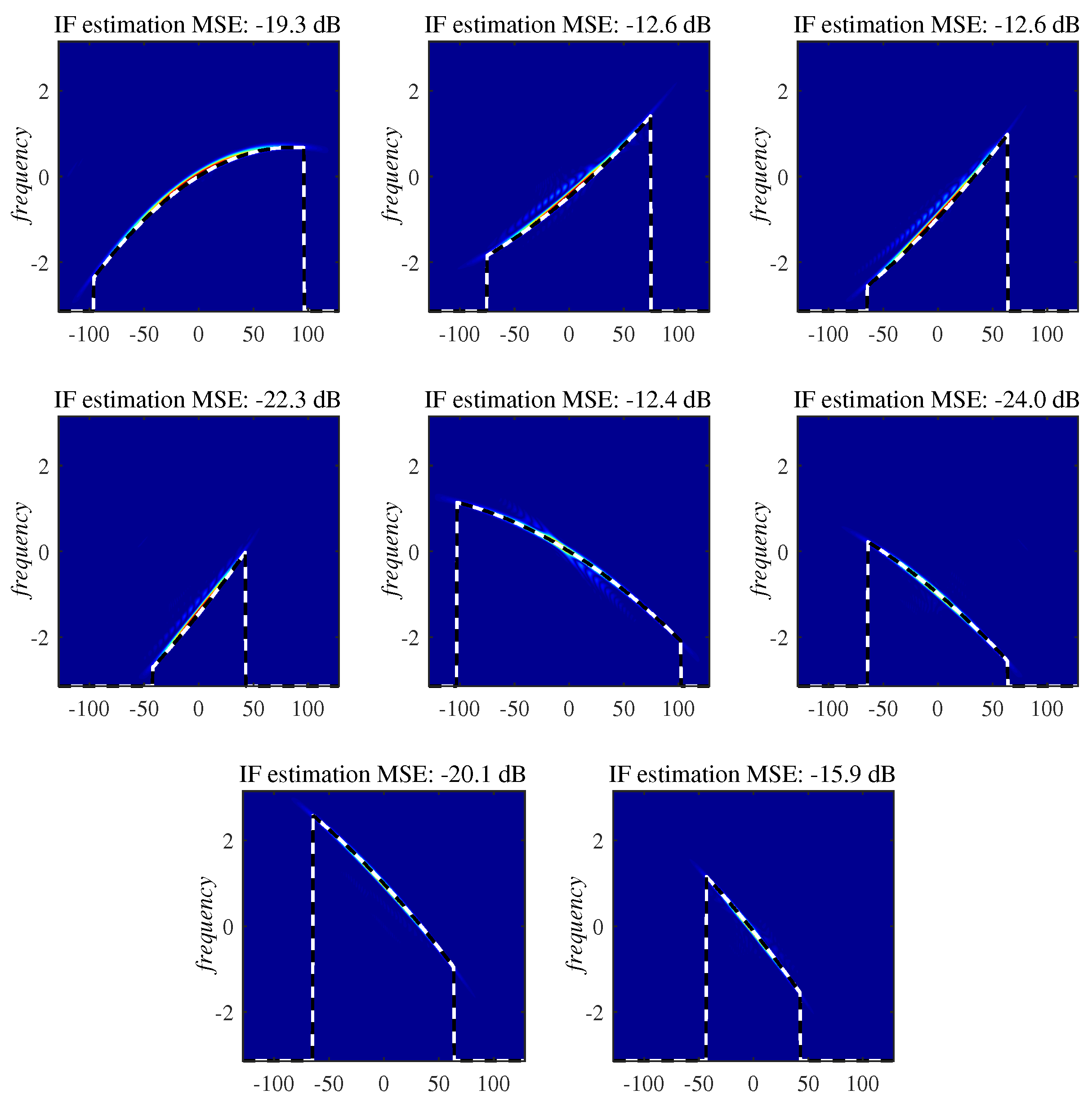
For examples 1, 2, and 3, the quality of the decomposition will be determined based on two criteria:

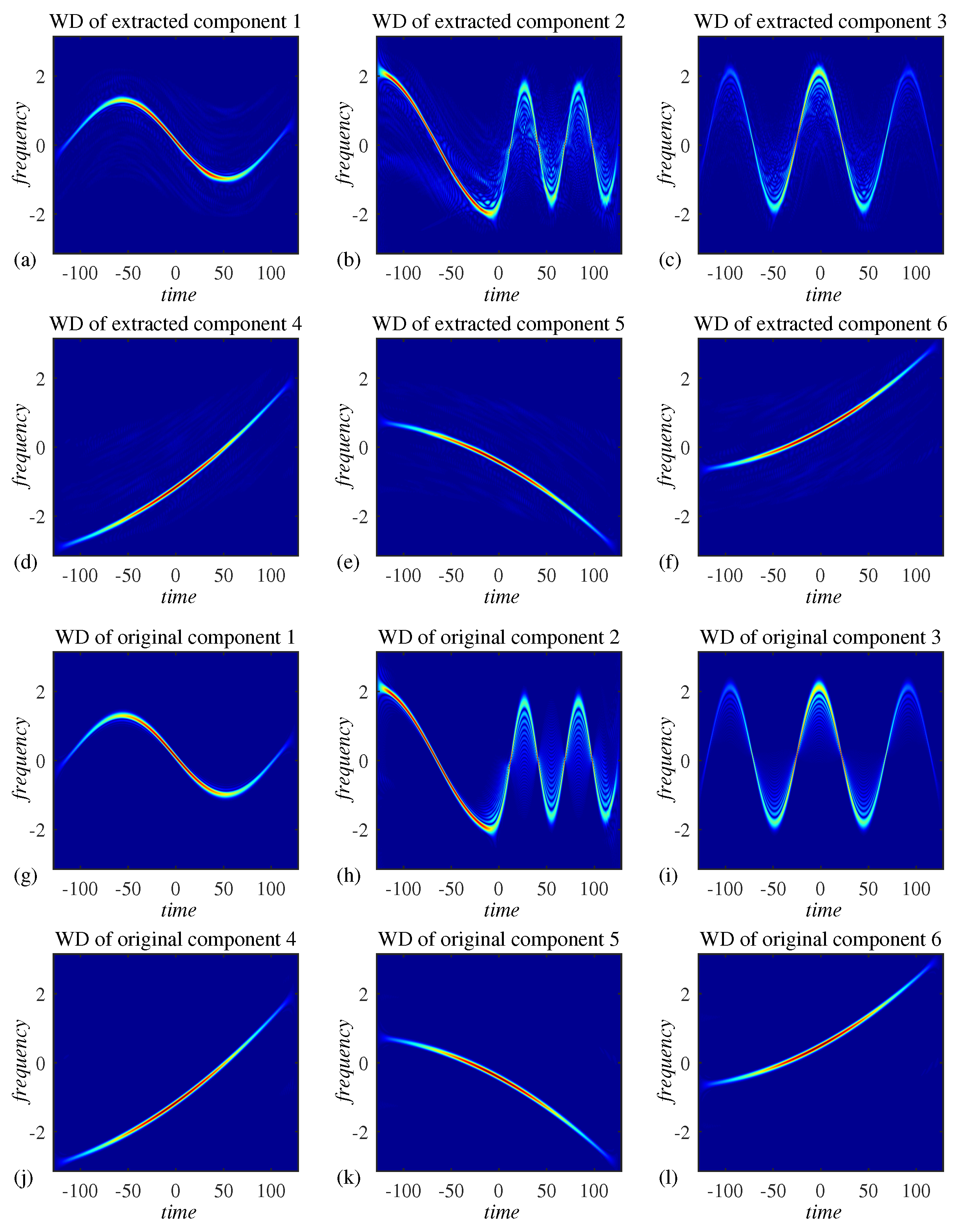
• WD calculated for the pth original component (signal is given analytically), denoted by $W{D}_p^o(n,k)=WD\left\{{\mathbf{s}}_p\right\}$, is compared with $W{D}_p^e(n,k)=WD\left\{{\widehat{\mathbf{s}}}_p\right\}$, being the WD calculated for pth extracted component, for $p=1,2,\cdots ,P$. Here, $\widehat{\mathbf{s}}$ denotes the vector of the pth extracted component, whereas ${\mathbf{s}}_p$ is the actual (original) pth signal component.
• Estimation results for the discrete IFs obtained from the two previous WDs are compared by the means of mean squared error (MSE) for each pair of components. The IF estimate based on the WD of the original pth component, $W{D}_p^o(n,k)$, $p=1,2,\cdots ,P$ is calculated as [3]

  $$k_p^o\left(n\right)=arg\underset{k}{max}W{D}_p^o(n,k)$$

  (54)

  whereas the IF estimate based on the WD of the pth component extracted by the proposed approach is calculated as

  $$k_p^e\left(n\right)=arg\underset{k}{max}W{D}_p^e(n,k).$$

  (55)
  Since the extracted components do not have any particular order after the decomposition is finished, the corresponding pairs of original and extracted components are automatically determined using the following procedure:
  • For p in $1,2,\cdots ,P$ repeat steps (a)–(f)

    (a)

    Calculate $k_p^o\left(n\right)$ based on (54) for analytically defined component ${\mathbf{s}}_p$.

    (b)

    Run decomposition algorithm. Use only eigenvectors corresponding to the largest P eigenvalues. Each of these eigenvectors, ${\mathbf{q}}_p$, contain an extracted signal component. If P is not given, estimate the number of components, P, as the number of eigenvalues, ${\lambda }_p$, of matrix $\mathbf{R}$, larger than threshold $T={\sigma }_{\epsilon }^2+{10}^{-4}$.

    (c)

    Initialize set $\mathbb{E}\leftarrow \varnothing$, to store the errors between IFs estimated based on the given original component ${\mathbf{s}}_p$ and extracted (unordered) components ${\mathbf{q}}_i$, $i=1,2,\cdots ,P$, being the outputs of the decomposition procedure.

    (d)

    For each extracted component, ${\mathbf{q}}_1,{\mathbf{q}}_2,\cdots ,{\mathbf{q}}_P$ repeat steps i–iii:

    • Calculate the IF estimate $k_i^e\left(n\right)$ as:

      $$k_i^e\left(n\right)\leftarrow arg\underset{k}{max}WD\left\{{\mathbf{q}}_i\right\}.$$
    • Calculate mean squared error (MSE) between $k_p^o\left(n\right)$ and $k_i^e\left(n\right)$ as

      $$MSE\left(i\right)\leftarrow \frac{1}{N}\sum _{n=0}^{N-1}{\left|k_p^o\left(n\right)-k_i^e\left(n\right)\right|}^2.$$
    • $\mathbb{E}\leftarrow \mathbb{E}\cup MSE\left(i\right)$.

    (e)

    $\widehat{p}\leftarrow arg{min}_{i}MSE\left(i\right)$

    (f)

    ${\widehat{\mathbf{s}}}_p\leftarrow {\mathbf{q}}_{\widehat{p}}$ is the pth estimated component, corresponding to the original component ${\mathbf{s}}_p$.

Upon determining pairs of original and estimated components, $({\mathbf{s}}_p,{\widehat{\mathbf{s}}}_p)$, respective IF estimation MSE is calculated for each pair

$$MS{E}_p=\frac{1}{N}\sum _{n=0}^{N-1}{\left|k_p^o\left(n\right)-k_p^e\left(n\right)\right|}^2,p=1,2,\cdots ,P,$$

(56)

where $k_p^e\left(n\right)=arg{max}_{k}WD\left\{{\widehat{\mathbf{s}}}_p\right\}$.

It should also be noted that in Examples 1–3, in order to avoid IF estimation errors at the ending edges of components (since they are characterized by time-varying amplitudes), the IF estimation is based on the WD auto-term segments larger than $10\%$ of the maximum absolute value of the WD corresponding to the given component (auto-term), i.e.,

$${\widehat{k}}_p^o\left(n\right)=\left\{\begin{array}{cc}{k}_p^o\left(n\right),\hfill & \mathrm{for}|W{D}_p^o(n,k)|\ge T_{W{D}^o},\hfill \\ 0,\hfill & \mathrm{for}|W{D}_p^o(n,k)|<T_{W{D}^o},\hfill \end{array}\right.$$

(57)

where $T_{W{D}^o}=0.1max\left\{\right|W{D}_p^o(n,k)\left|\right\}$ is a threshold used to determine whether a component is present at the considered instant n. If it is smaller than $10\%$ of the maximal value of the WD, it indicates that the component is not present.

Examples

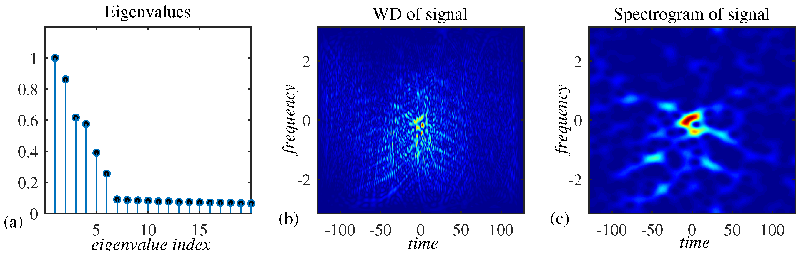
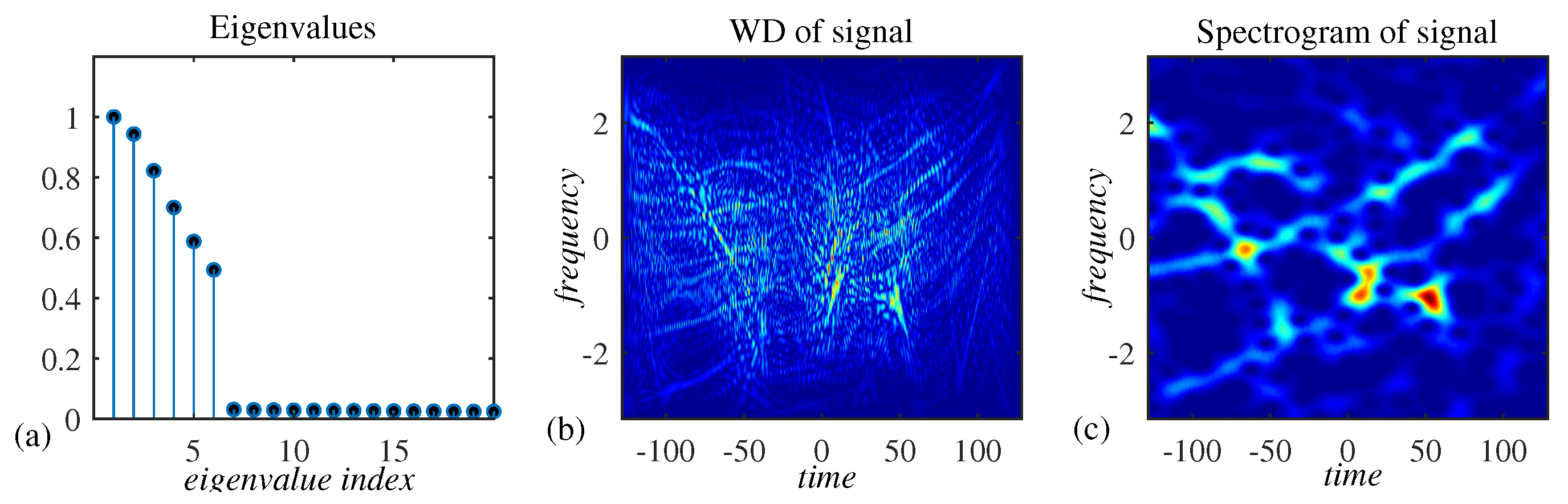
Example 1.

To evaluate the presented theory, we consider a general form of a multicomponent signal consisted of P non-stationary components

$$x_p^{\left(c\right)}\left(n\right)=\sum _{p=1}^P{A}_{p}exp\left(-\frac{n^2}{L_p^2}\right)exp\left(j\frac{1}{N^2}{n}^3+j\frac{2\pi f_p}{N}{n}^2+j\frac{2\pi {\varphi }_p}{N}n+j{\vartheta }_c\right)+{\epsilon }^{\left(c\right)}\left(n\right),$$

(58)

$-128\le n\le 128$ and $N=257$. Phases ${\vartheta }_c$, $c=1,2,\cdots ,C$, are random numbers with uniform distribution drawn from interval $\left[-\pi ,\pi \right]$. The signal is available in the multivariate form $\mathbf{x}\left(n\right)={\left[x^{\left(1\right)}\left(n\right),x^{\left(2\right)}\left(n\right),\cdots ,x^{\left(C\right)}\left(n\right)\right]}^T,$ and is consisted of C channels, since it is embedded in a complex-valued, zero-mean noise ${\epsilon }^{\left(c\right)}\left(n\right)$ with a normal distribution of its real and imaginary part, $\mathcal{N}(0,{\sigma }_{\epsilon }^2)$. Noise variance is ${\sigma }_{\epsilon }^2$, whereas $A_p=1.2$. Parameters $f_p$ and ${\varphi }_p$ are FM parameters, while $L_p$ is used to define the effective width of the Gaussian amplitude modulation for each component.

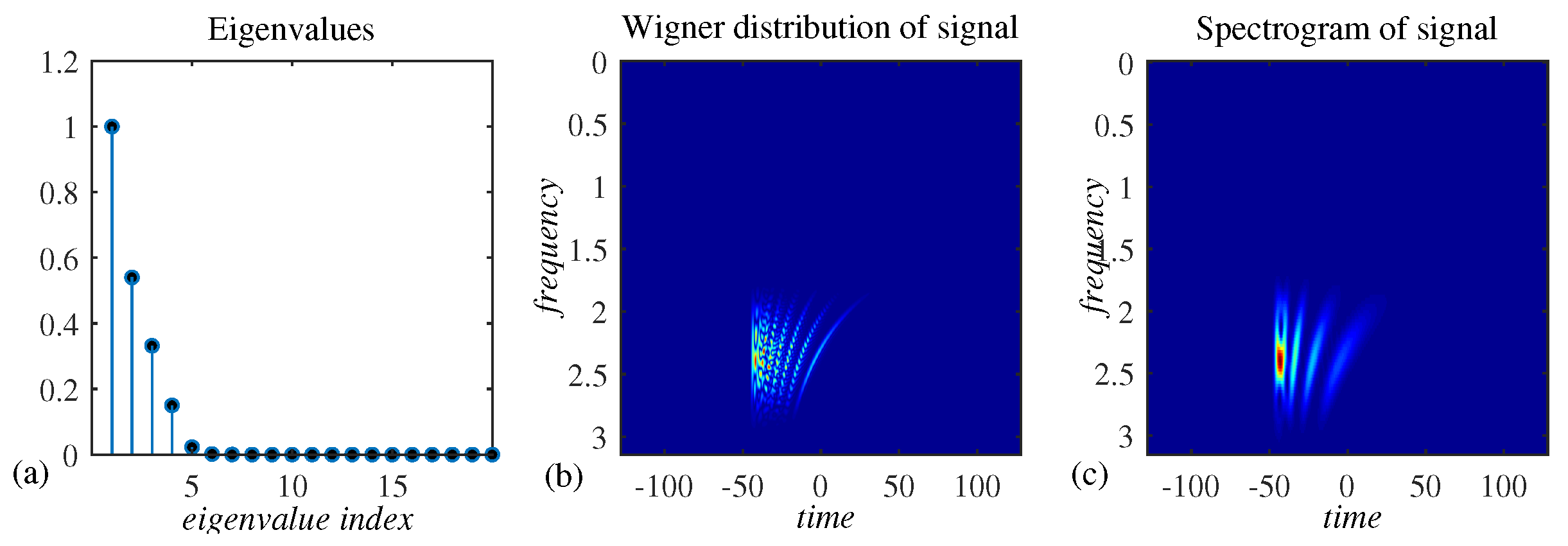
We generate the signal of the form (58) with $P=6$ components, whereas the noise variance is ${\sigma }_{\epsilon }=1$. The respective number of channels is $C=128$. The corresponding autocorrelation matrix, $\mathbf{R}$, is calculated, according to (20), and the presented decomposition approach is used to extract the components. Eigenvalues of matrix $\mathbf{R}$ are given in Figure 2a. Largest six eigenvalues correspond to signal components, and they are clearly separable from the remaining eigenvalues corresponding to the noise. WD and spectrogram of the given signal (from one of the channels) are given in Figure 2b,c, indicating that the signal is not suitable for the classical TF analysis, since the components are highly overlapped.

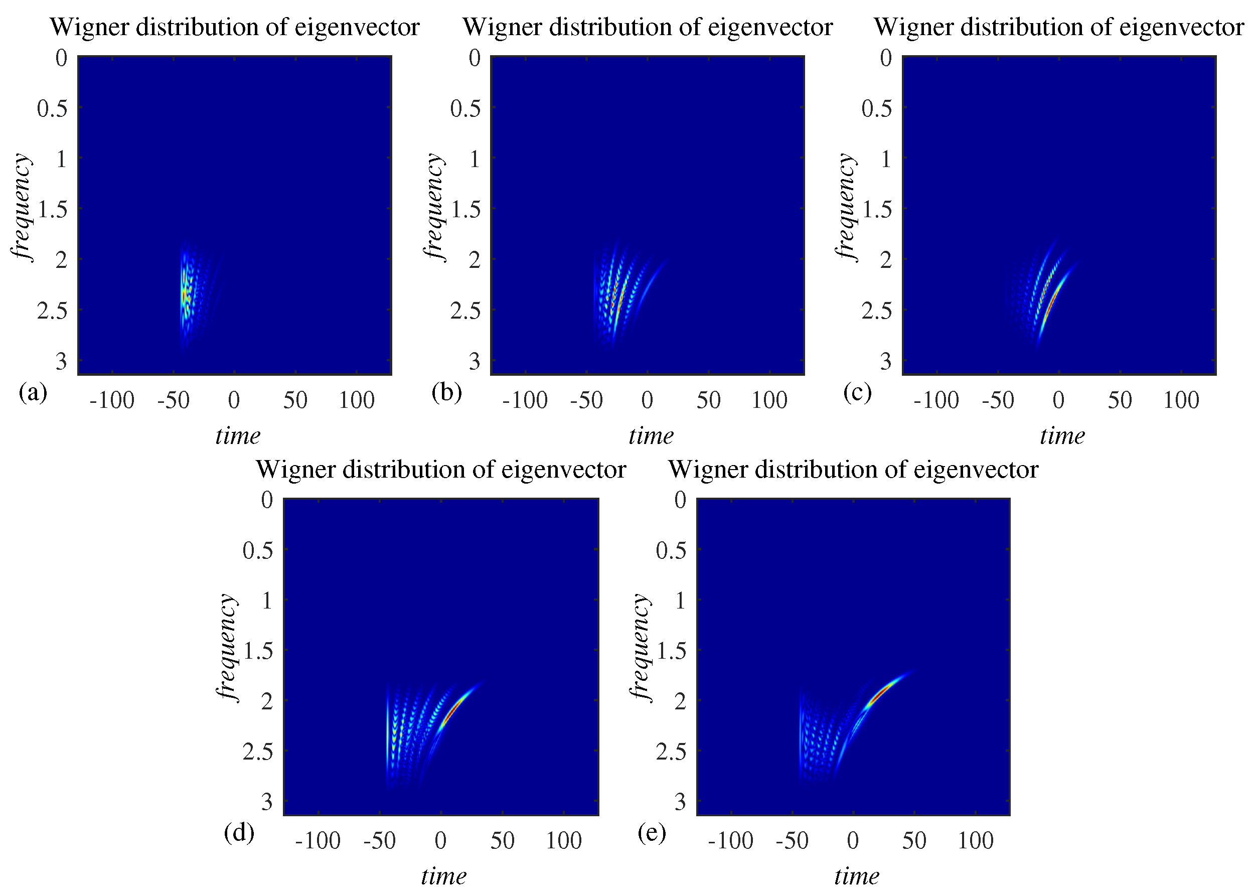
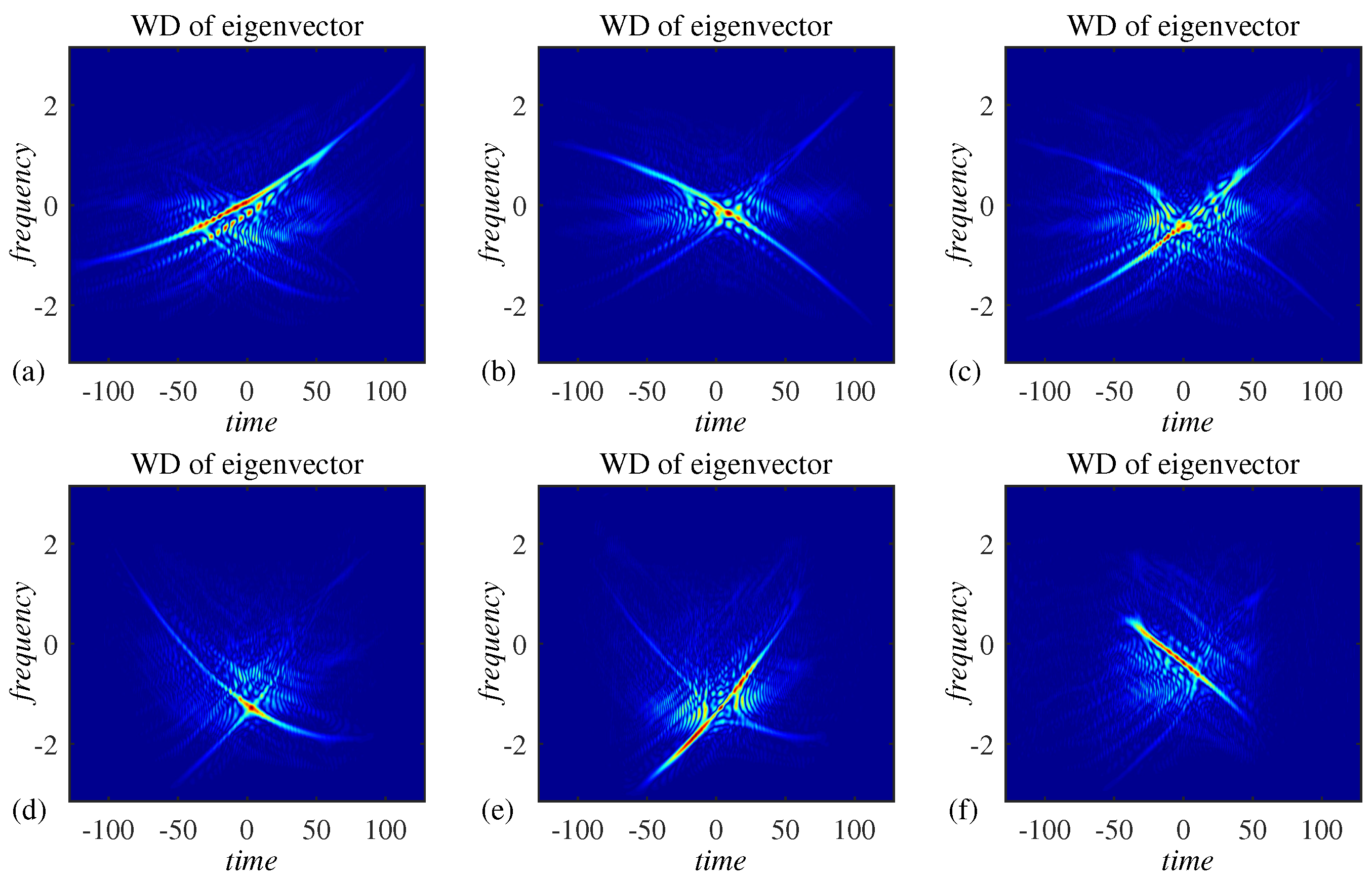
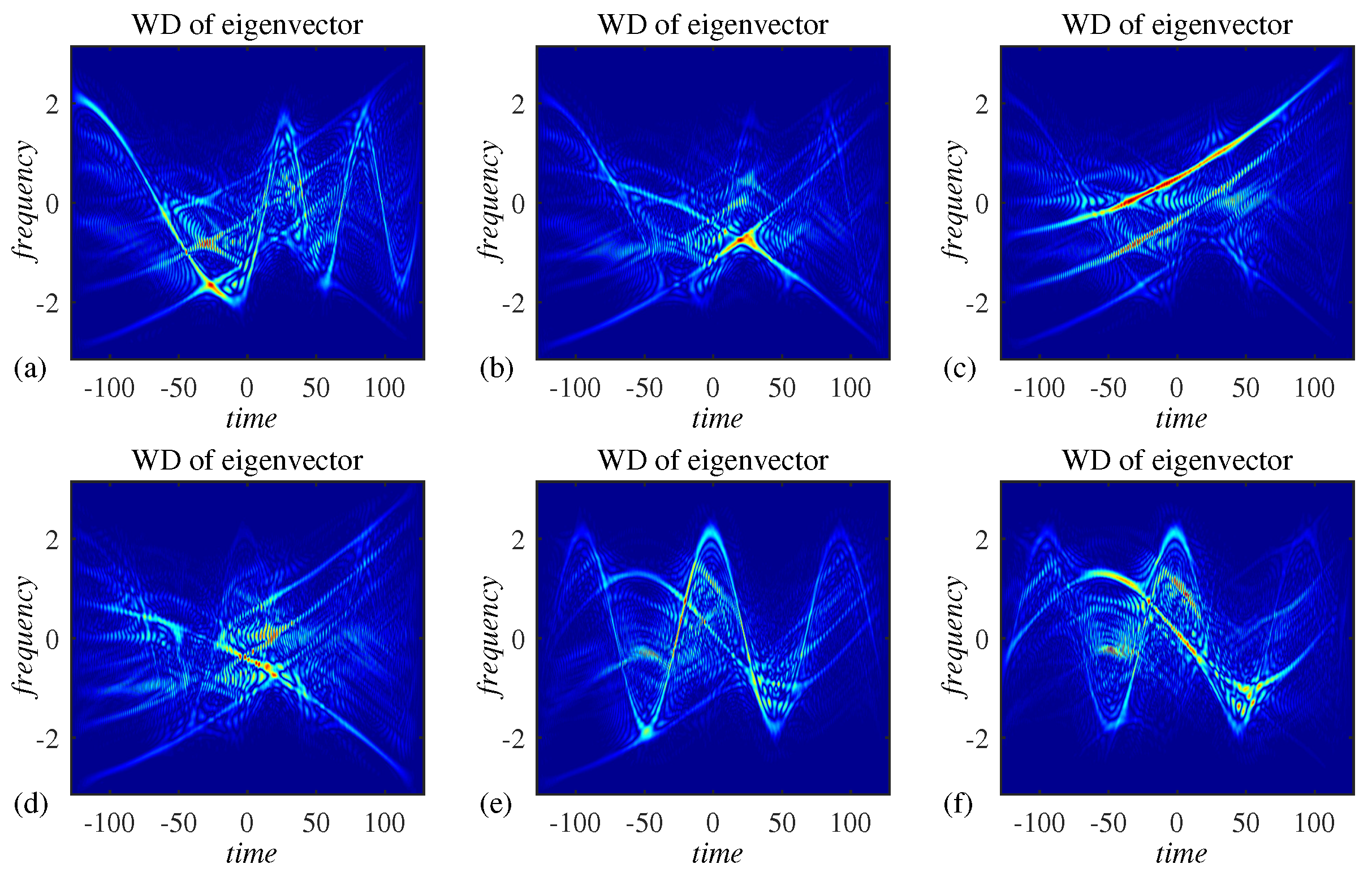
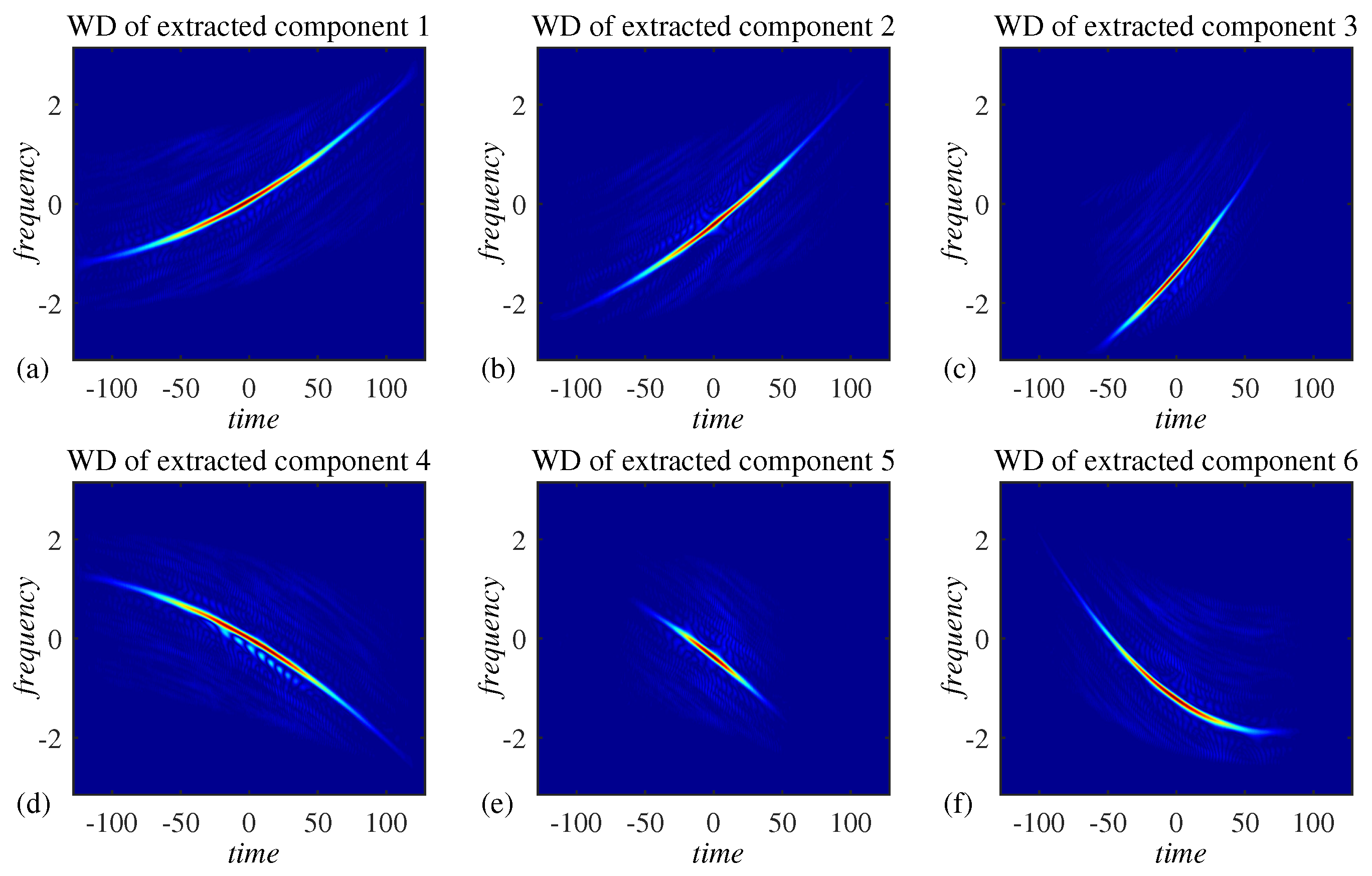
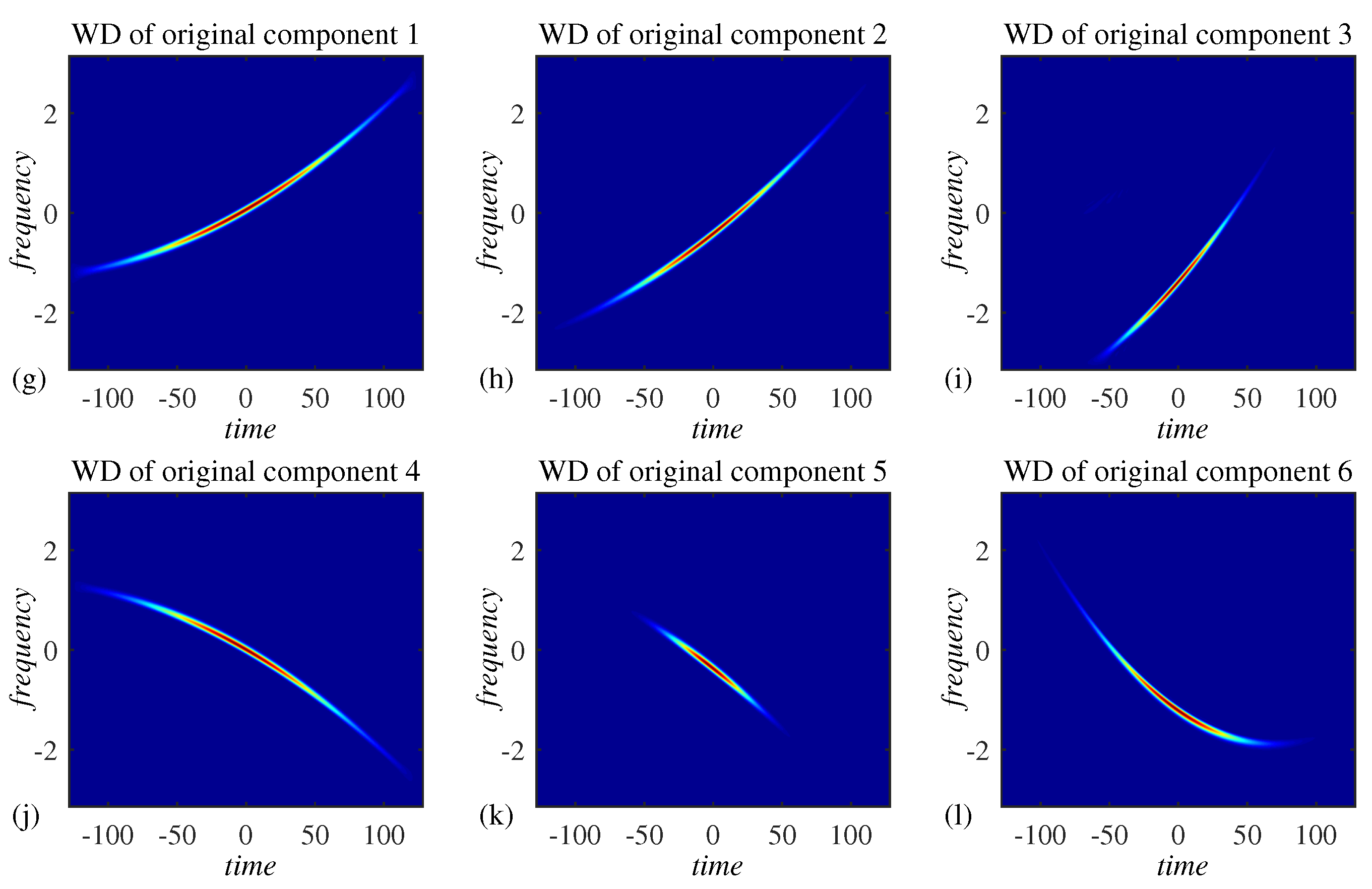
Each of eigenvectors of the matrix $\mathbf{R}$ is a linear combination of components, as shown in Figure 3. The presented decomposition approach is applied to extract the components by linearly combining the eigenvectors from Figure 3. The results are shown in Figure 4a–f. Although a small residual noise is present in the extracted components, they highly match the original components, presented in Figure 4g–l. The original components in Figure 4g–l are not corrupted by the noise.

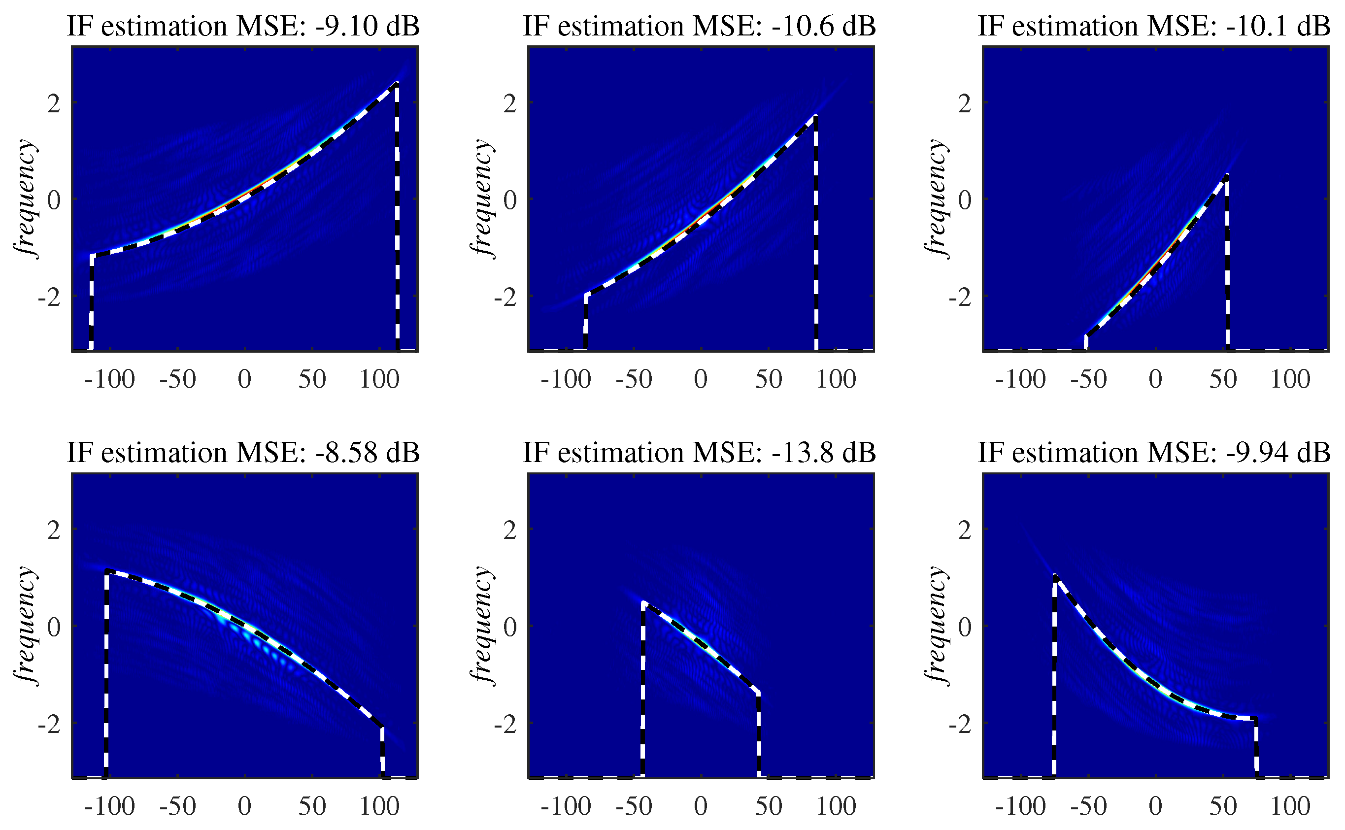
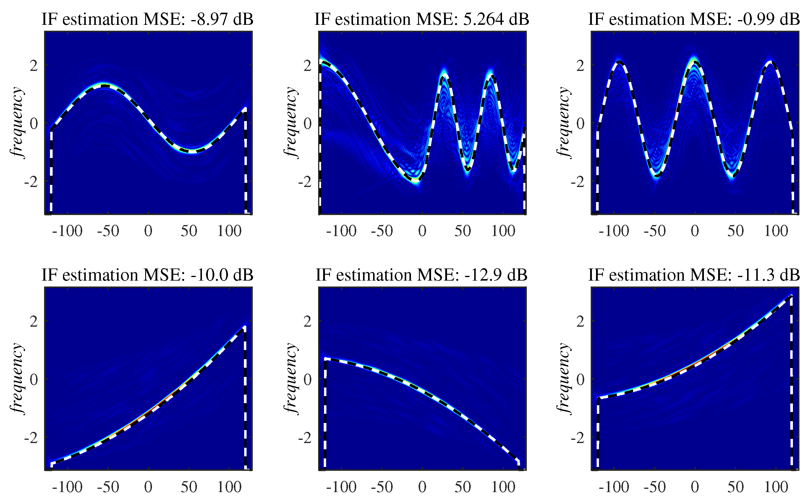
As a measure of quality, we engage $MS{E}_p$ given by (56), which is the error between the IF estimation result based on the pth extracted signal component (shown in Figure 4a–f) versus the IF estimation calculated based on the WD of original, noise-free component (from Figure 4g–l). The IF estimates and the corresponding MSEs are, for each pair of components, presented in Figure 5, for standard deviation of the noise ${\sigma }_{\epsilon }=1$, where the number of channels is $C=128$.

Since $MS{E}_p$ given by (56) serves as a measure of the component extraction quality, we evaluate the decomposition performance for various standard deviations of the noise, ${\sigma }_{\epsilon }\in \left\{0.1,0.4,0.7,1.0,1.3,1.9,2.1\right\}$. Results are presented in

Table 1. Mean squared errors (MSEs) between IF estimations based on extracted and original components, for signal from Example 1 with $P=6$ components. $MS{E}_p$, $p=1,2,\cdots ,6$ corresponds to the pth component. The results are presented for various values of the standard deviation of the noise, ${\sigma }_{\epsilon }$. The results are averaged based on 10 random realizations of signals with random phases and noise, for each considered value of ${\sigma }_{\epsilon }$.

${\sigma }_{\epsilon }$	${MSE}_1$	${MSE}_2$	${MSE}_3$	${MSE}_4$	${MSE}_5$	${MSE}_6$
0.1	−20.89 dB	−16.12 dB	−18.67 dB	−15.66 dB	−11.86 dB	−22.65 dB
0.4	−16.63 dB	−14.52 dB	−11.19 dB	−12.44 dB	−10.22 dB	−17.21 dB
0.7	−20.89 dB	−12.23 dB	−12.04 dB	−12.04 dB	−9.13 dB	−15.66 dB
1.0	−13.62 dB	−10.89 dB	−7.27 dB	−10.22 dB	−6.21 dB	−12.04 dB
1.3	−12.65 dB	−9.86 dB	−7.46 dB	−9.53 dB	−3.99 dB	−13.62 dB
1.6	−9.63 dB	16.67 dB	35.04 dB	−10.74 dB	27.28 dB	36.01 dB
1.9	−9.75 dB	32.50 dB	39.85 dB	−12.87 dB	30.28 dB	34.61 dB
2.1	−9.86 dB	−7.33 dB	−8.42 dB	−9.64 dB	7.03 dB	−7.46 dB

. The presented MSEs are calculated by averaging the results obtained based on 10 realizations of multichannel signal of the form (58) with random phases ${\vartheta }_c$, $c=1,2,\cdots ,C$ and corrupted by random realizations of the noise ${\epsilon }^{\left(c\right)}\left(n\right)r$, for each observed variance (standard deviation) of the noise. Based on the results from Table 1, it can be concluded that each signal component is successfully extracted for noise characterized by standard deviation up to ${\sigma }_{\epsilon }=1.3$. For stronger noise, only some components are successfully extracted. It shall be noted that the performance of the algorithm depends also on the number of channels, C. For the results from Table 1, the number of channels was set to $C=256$. A larger value of C increases the probability of successful decomposition, as investigated in [31].

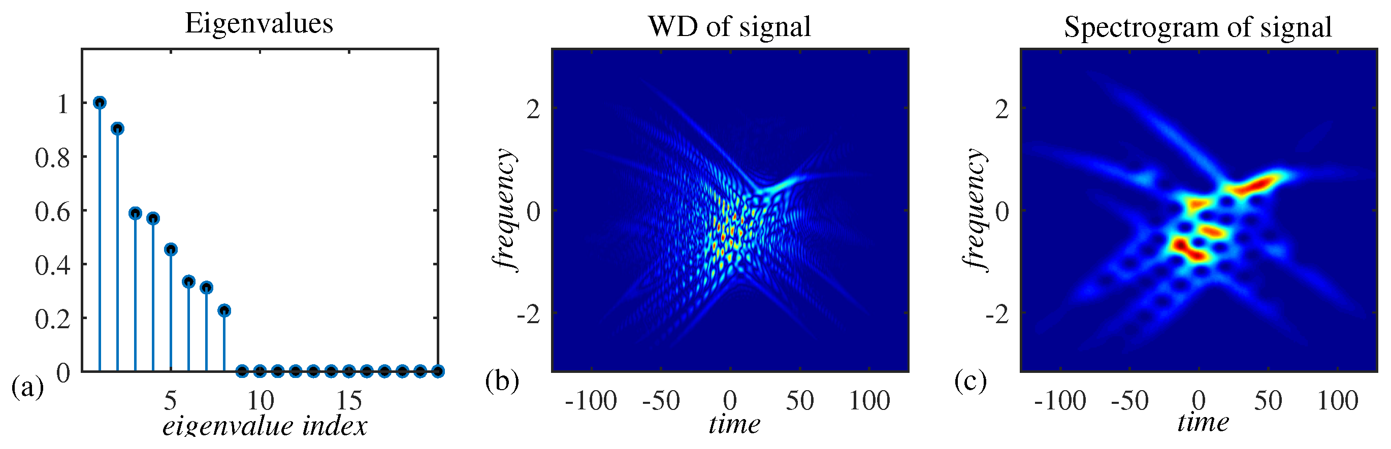
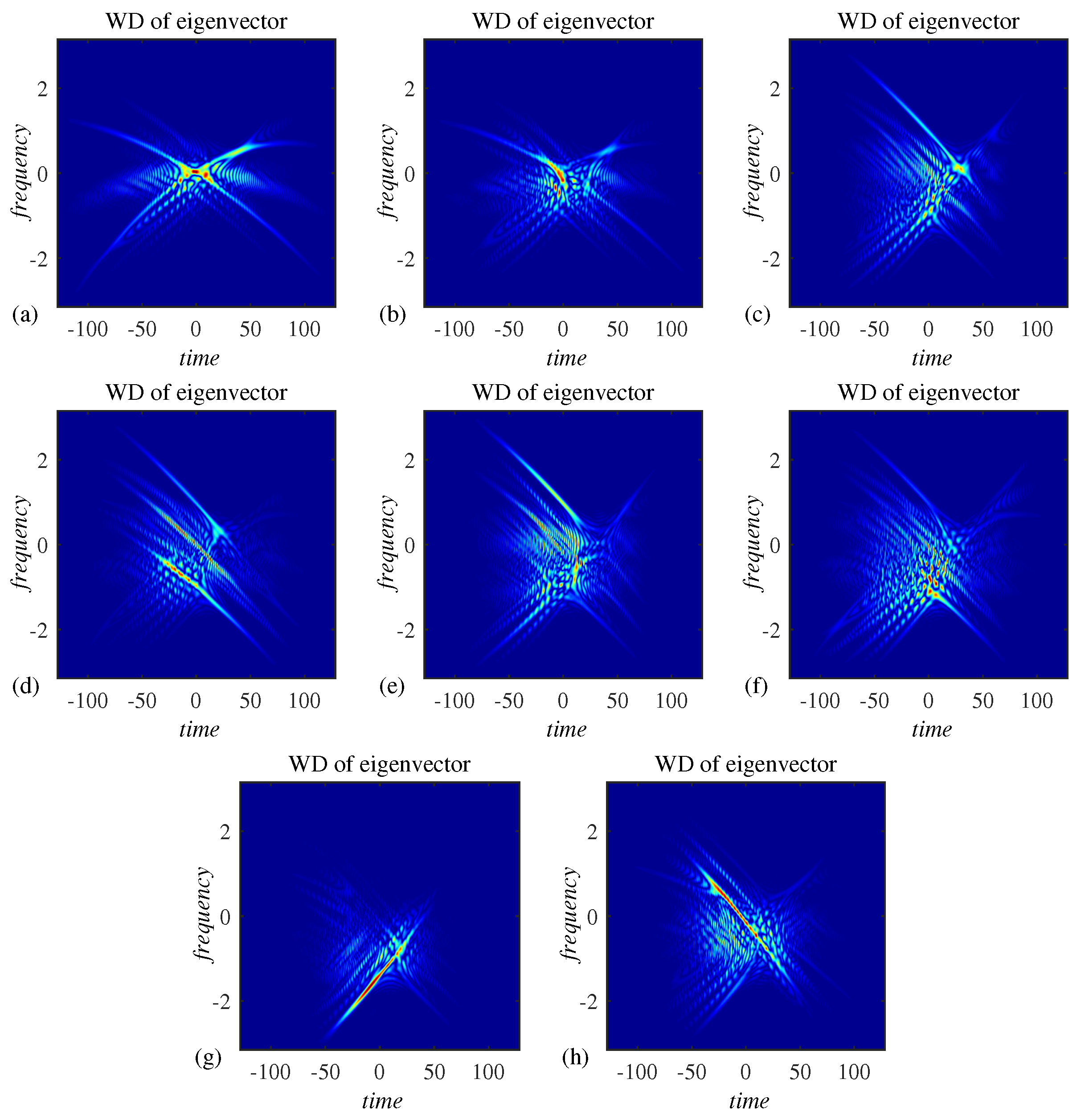
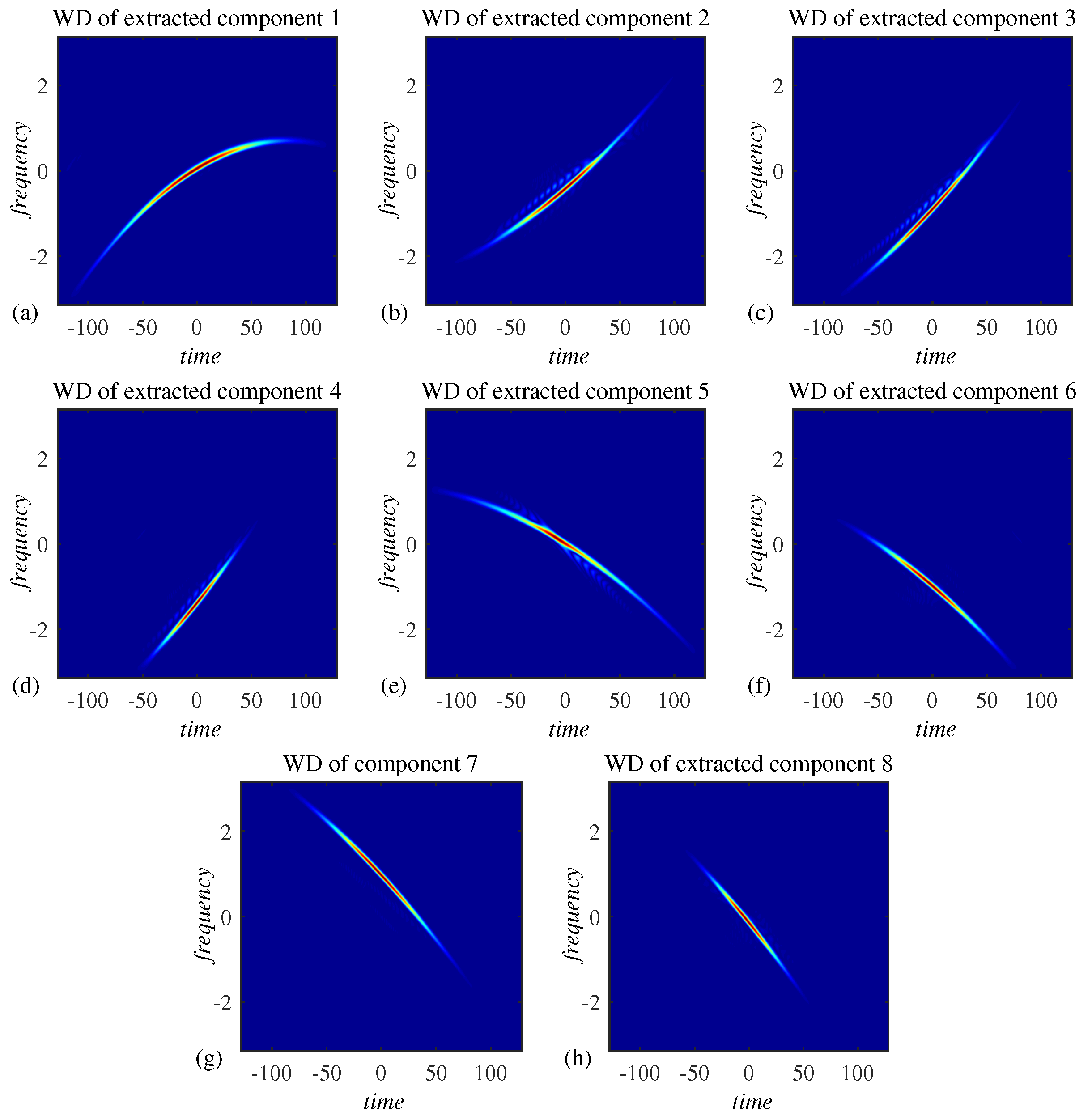
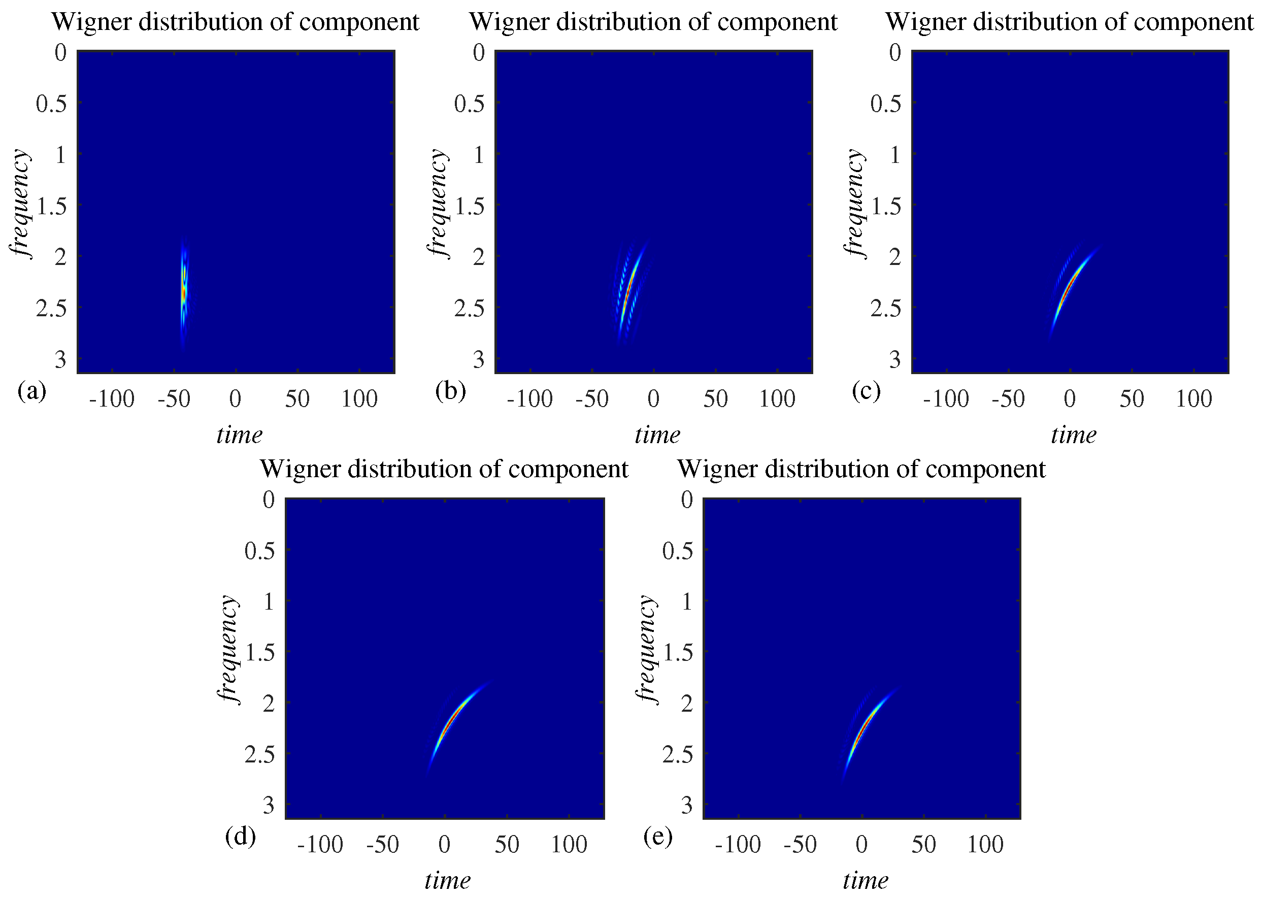
Example 2.

The decomposition algorithm is tested on a more complex signal of the form (58), with $P=8$ components, whereas the standard deviation of the noise is now ${\sigma }_{\epsilon }=0.1$. The number of channels is $C=128$. After the input autocorrelation matrix, $\mathbf{R}$, is calculated, according to (20), eigendecomposition produced the eigenvalues given in Figure 6a. Signal components overlap in the time-frequency domain and, therefore, the corresponding Wigner distribution and spectrogram shown in Figure 6b,c cannot be used as adequate tools for their analysis. Figure 7 indicates that the components are neither visible in the time-frequency representation of any eigenvector corresponding to the largest eigenvalues. This is in accordance with the fact that eigenvectors contain signal components in the form of their linear combinations. Upon applying the presented multivariate decomposition procedure on this set of eigenvectors, we obtain results presented in Figure 8. By comparing the results with Wigner distributions of individual, noise-free components, shown in Figure 9, comprising the considered multicomponent signal, it can be concluded that the components are successfully extracted with preserved integrity. This is additionally confirmed by the IF estimation results shown in Figure 10, where even lower MSE values for each component can be explained by the lower noise level, as compared with results from the previous example.

Example 3.

To illustrate the applicability of the presented approach in decomposition of components with faster or progressive frequency variations over time, we observe a signal consisted of $P=6$ components, three of which have polynomial modulations as components in model (58), whereas three other components have frequency modulations of sinusoidal nature. The first three components are defined as:

$$s_1^{\left(c\right)}\left(n\right)=exp\left(-{\left(n/128\right)}^2\right)exp\left(j40.5cos\left(2.34\pi n/N\right)+j10\pi n/N+j{\vartheta }_c\right)$$

(59)

$$s_2^{\left(c\right)}\left(n\right)=\left\{\begin{array}{cc}exp\left(j16sin\left(9\pi n/N\right)+j{\vartheta }_c\right),\hfill & \mathrm{for}\ge 0\hfill \\ exp\left(j85.33sin\left(2\pi (n+128)/N\right)+j{\vartheta }_c\right),\hfill & \mathrm{for}n<0\hfill \end{array}\right.$$

(60)

$$s_3^{\left(c\right)}\left(n\right)=exp\left(-{\left(n/128\right)}^2\right)exp\left(j30.5sin\left(5.47\pi n/N\right)+j10\pi n/N+j{\vartheta }_c\right)$$

(61)

The remaining components have polynomial frequency modulation, as in previous examples:

$$s_p^{\left(c\right)}\left(n\right)=A_{p}exp\left(-\frac{n^2}{L_p^2}\right)exp\left(j\frac{1}{N^2}{n}^3+j\frac{2\pi f_p}{N}{n}^2+j\frac{2\pi {\varphi }_p}{N}n+{\vartheta }_c\right)+{\epsilon }^{\left(c\right)}\left(n\right)$$

(62)

for $p=4,5,6$. Again, the signal is defined for discrete indices $-128\le n\le 128$ and $N=257$ phases ${\vartheta }_c$, $c=1,2,\cdots ,C$, are random numbers with uniform distribution drawn from interval $\left[-\pi ,\pi \right]$. The resulting multicomponent signal is formed in cth channel as:

$$x_p^{\left(c\right)}\left(n\right)=\sum _{p=1}^6{s}_p^{\left(c\right)}\left(n\right)+{\epsilon }^{\left(c\right)}\left(n\right),$$

(63)

and is, as in previous examples, embedded in additive, white, complex-valued Gaussian noise, now with variance ${\sigma }_{\epsilon }=1$. The number of channels is $C=256$. Eigenvalues of the autocorrelation matrix $\mathbf{R}$, WD and spectrogram are given in Figure 11, again proving the that the considered signal with heavily overlapped components cannot be analyzed with these tools. Eigenvectors corresponding to the largest six eigenvalues are given in Figure 12. Extracted and original components can be visually compared in Figure 13, again proving the efficiency of the approach, even in the case for components with a faster varying frequency content. This is additionally confirmed by IF estimation results in Figure 14. Larger estimation errors when faster sinusoidal frequency modulations are present are related to poorer concentration of the WD in these cases [3].

Example 4.

In this example, we consider the dispersive environment setup described in Section 2.2, with the transmitter located in the water at the depth of $z_t$. However, to obtain a multivariate signal, instead of one sensor, $K=25$ sensors are placed at the depth $z_r$, comprising the receiver at distances $r+{\delta }_c$, $c=1,2,\cdots ,C$, from the transmitter. Moreover, the mutual sensor distances are negligible compared with their distance from the transmitter, $r=2000$ m; that is ${\delta }_c\ll r$. This further implies that the range direction remains unchanged in our model. As a response to a monochromatic signal $s\left(n\right)=exp\left(j{\omega }_{0}n\right)$, at sensor c, the linear combination of modes $s_p^{\left(c\right)}\left(n\right)=A_t(m,{\omega }_0)exp(j{\omega }_{0}n-j{k}_c(p,{\omega }_0)r)$ is received:

$$x^{\left(c\right)}\left(n\right)=\sum _{p=1}^P{s}_p^{\left(c\right)}\left(n\right)=\sum _{p=1}^P{A}_t(m,{\omega }_0)exp(j{\omega }_{0}n-j{k}_c(p,{\omega }_0)r),$$

(64)

where $c=1,2,\cdots ,C$, and wavenumbers are modeled as $k_c(m,\omega )$ [55]

$$k_r^2(m,\omega )={\left(\frac{\omega }{c}\right)}^2-{\left((m-0.5)\frac{\pi }{D+{\vartheta }_c}\right)}^2,$$

(65)

$D=20$ m and ${\vartheta }_c$ is a random variable drawn from interval $[-0.25,0.25]$ with uniform distribution; therefore, corresponding to depth variations of $\pm 0.25$ cm, modeling channel depth changes due to surface waves or uneven seabed. The speed of sound propagation underwater is $c=1500$ m/s. The same results in this example are obtained for a more precise speed, i.e., at $c=1480$ m/s. The received multichannel signal is of the form

$$\mathbf{x}\left(n\right)=\left[\begin{array}{c}{x}^{\left(1\right)}\left(n\right)\\ x^{\left(2\right)}\left(n\right)\\ ⋮\\ x^{\left(C\right)}\left(n\right)\end{array}\right].$$

(66)

Upon performing the eigenvalue decomposition of autocorrelation matrix $\mathbf{R}$, eigenvalues shown in Figure 15a are obtained. The Wigner distribution of the received signal is shown in Figure 15b, with very close and partially overlapped nodes. Wigner distributions of individual eigenvectors are shown in Figure 16a–e. The presented procedure for the decomposition of multicomponent signals successfully extracted the individual acoustic modes, as presented in Figure 17a–e. Such separated acoustic modes can be further analyzed; for example, their IF can be estimated and characterized.

6. Discussion

Decomposition of non-stationary multicomponent signals has been a long-term, challenging topic in time-frequency signal analysis [19,20,21,22,23,24,25,26,27,28,29,30,31,32,33,34]. Although decomposition of non-overlapping components can be done using the S-method relations with the WD [26], this approach cannot be applied when the components partially overlap, i.e., share the same domain of support in the time-frequency plane.

Other alternative methodologies are specialized for some specific signal classes, and are efficient in the case of partially overlapped components [20,25,27]. In this sense, chirplet and Radon transform-based decomposition is applicable for linear frequency modulated signals [20,25]. Inverse Radon transform has produced excellent results in separation of micro-Doppler appearing in radar signal processing, characterized by a sinusoidal frequency modulation and periodicity [27]. However, outside the scope of their predefined signal models, these techniques are inefficient in separation of non-stationary signals characterized by some different laws of non-stationarity. Another very popular concept, namely the EMD, has been also applied multivariate data [39,40,41,42,43]. However, successful EMD-based multicomponent signal decomposition is possible only for signals having non-overlapping components in the TF plane. Amplitude variations of components pose an additional challenge to the EMD-based decomposition. The efficiency of the proposed method does not depend on the considered frequency range, but only on the ability of a time-frequency representation to concentrate signal components in the time-frequency plane. We use the STFT in concentration measure (31) due to its ability to concentrate signal energy at the instantaneous frequency of individual signal components. The decomposition approach studied in this paper successfully extracts components highly overlapped in the time-frequency plane. The method is not sensitive to the extent of overlap of the signal components.

Since the modes appearing in the considered acoustic dispersive environment framework are characterized by a non-linear (and non-sinusoidal) law of frequency variations and have a partially overlapped support, neither of the mentioned univariate techniques can produce acceptable decomposition results.

7. Conclusions

Characterization of modes in the acoustic dispersive environment is an ongoing research topic. As modes are non-stationary and present in a multicomponent form in the received signals, their separation (extraction) has been a challenging task. In this paper, we have shown that the modes can be successfully extracted based on a multivariate decomposition technique that exploits the eigenanalysis of the autocorrelation matrix of the received signal. This method, which utilizes concentration measures calculated based on time-frequency representations, separates the modes while completely preserving their integrity, thus opening the possibility for their individual analysis. IF estimations based on extracted components were highly accurate, even for a high level of noise. Results indicate that the efficiency of the method is increased with the larger number of sensors (channels). Our future work will be oriented towards the analysis of the separated components. Instantaneous frequency estimation techniques developed within the time-frequency signal analysis field can be applied directly on separated modes, providing new insights and tools for the analysis of dispersive channels.