
A New Extended Cosine—G Distributions for Lifetime Studies


 ,
,  and
and 
Abstract
:1. Introduction
2. The ECSG Family
2.1. Presentation
- Clearly, when , the ECSG family was reduced to the SG family.
- The pdf of the ECSG family is a weighted version of the pdf of the SG family; indeed, if we denoted the pdf of the SG family by , we could write:where . We, thus, saw how the parameter modulated the functionalities of , and the strong relationship existing with the respective pdfs. Naturally, the presence of the weight function completely modified the analytical structure of ; the mode and tail properties of truly depend on the variations of .
- When is a positive integer, is the cdf of the random variable , where are independent random variables with the cdf of the SG family. Thus, the ECSG family has an interpretation in terms of the distribution of minimum of several random variables.
- The function increased with respect to . This implies a first-order stochastic dominance with the SG family, which differs in nature according to and .
- More secondary, since , we could rewrite as:
2.2. Asymptotic Study
2.3. Quantile Function
2.4. Functional Series Representation
2.4.1. For the cdf
2.4.2. For the pdf
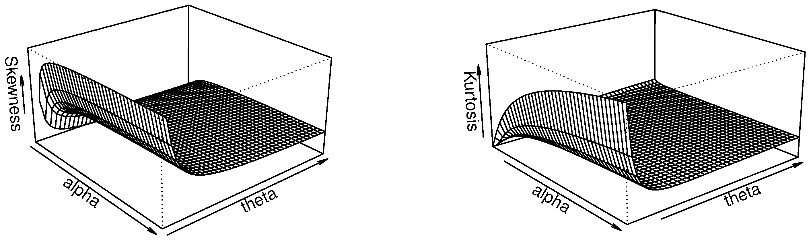
2.5. Moments
2.6. Reliability
2.7. Order Statistics
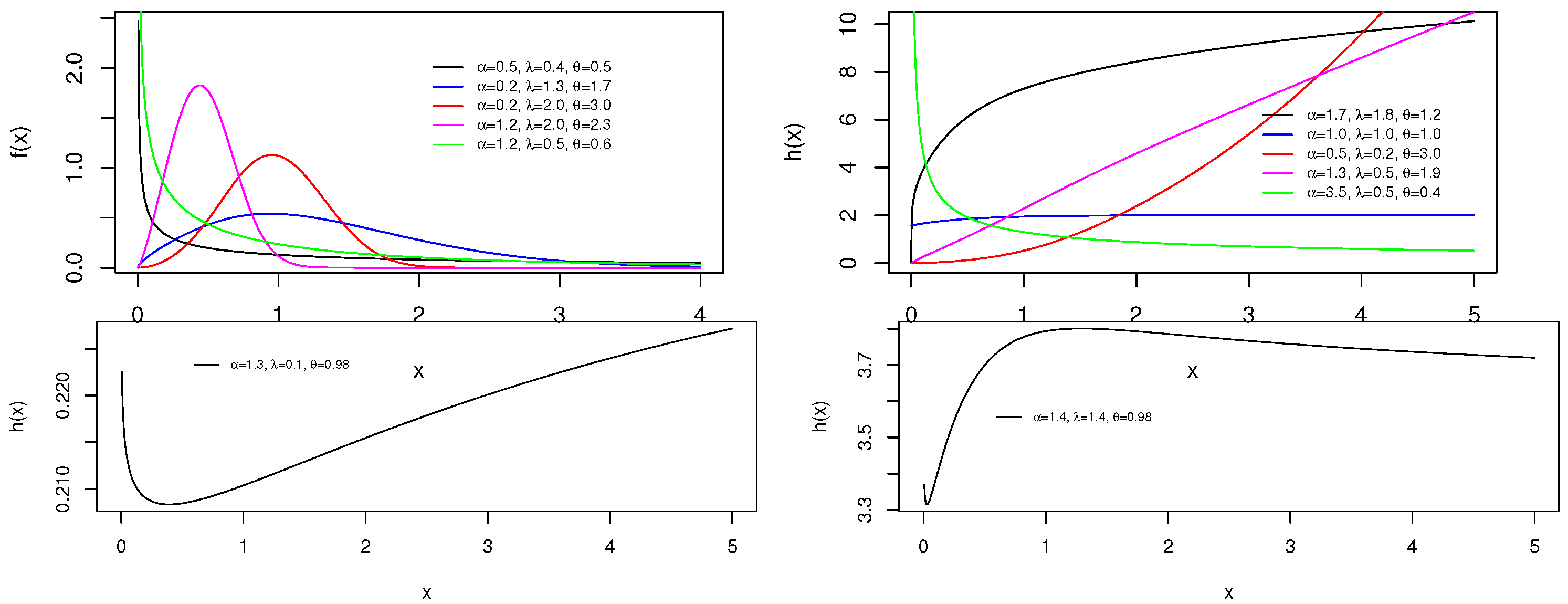
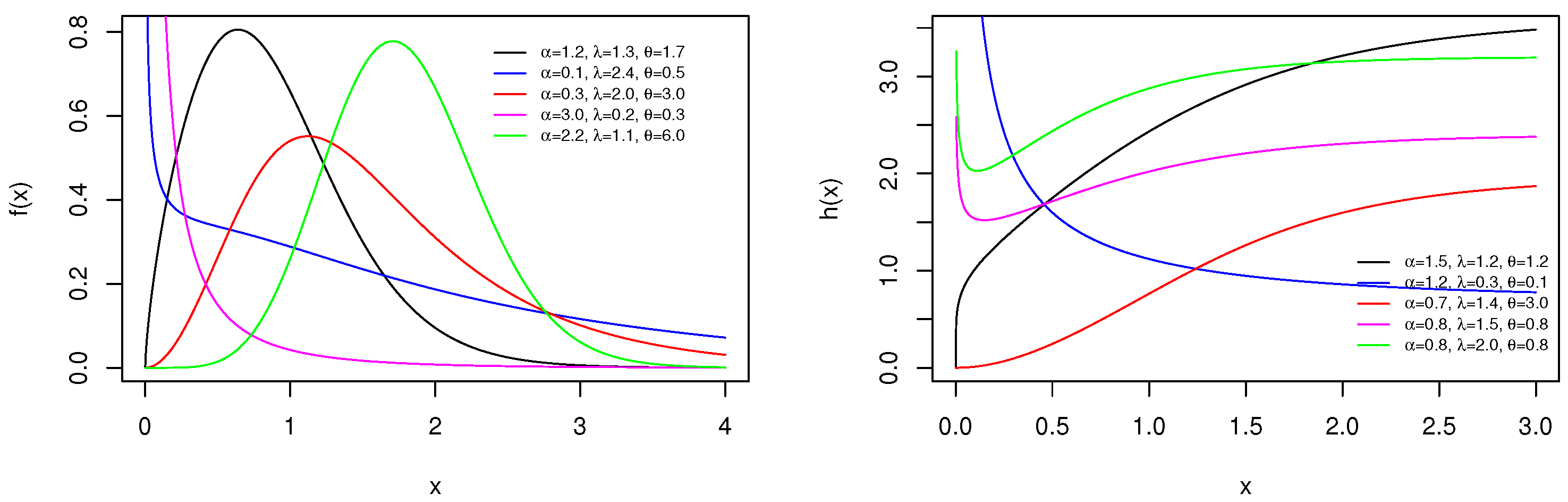
2.8. Special Members of the ECSG Family
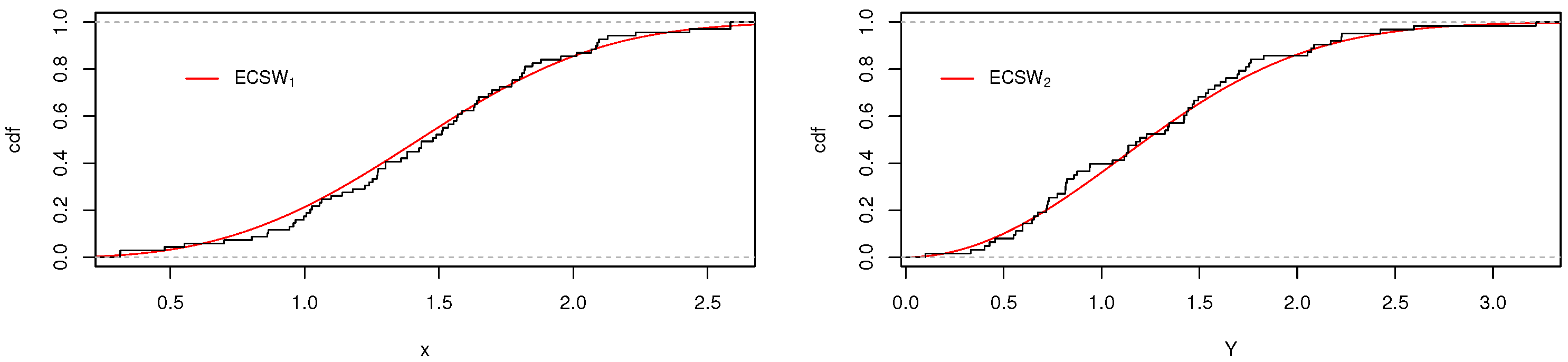
2.8.1. The ECSW Distribution
- As , the mean residual life of X satisfieswhere is the upper incomplete gamma function,
- As , the mean reverse residual life of X satisfies
- Suppose that . Let where and , then:for . The cdf of the standard Gumbel distribution was obtained as limit; converged in distribution to a random variable with such a Gumbel distribution.
- Let , where and , then:for . The cdf of the W distribution of parameters 1 and θ was obtained as limit; converged in distribution to a random variable with such a W distribution.
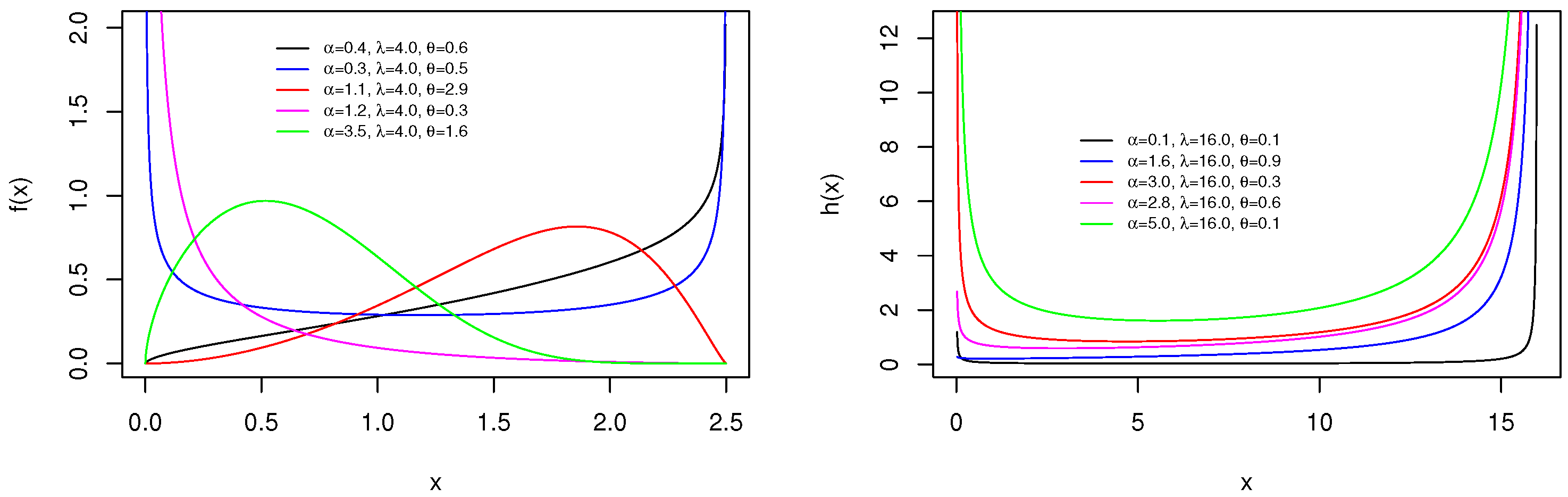
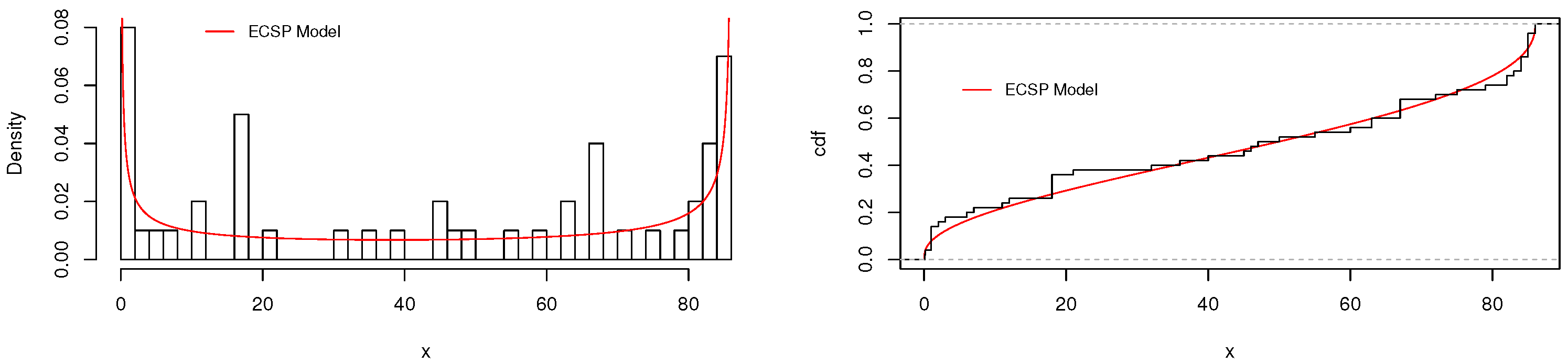
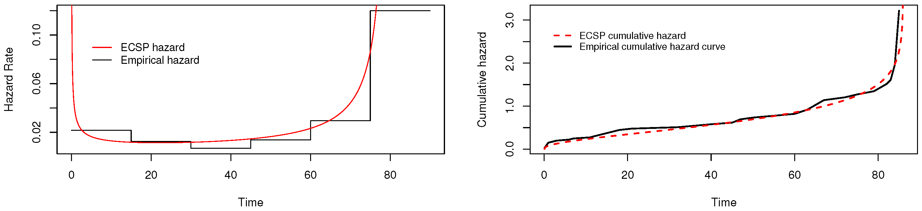
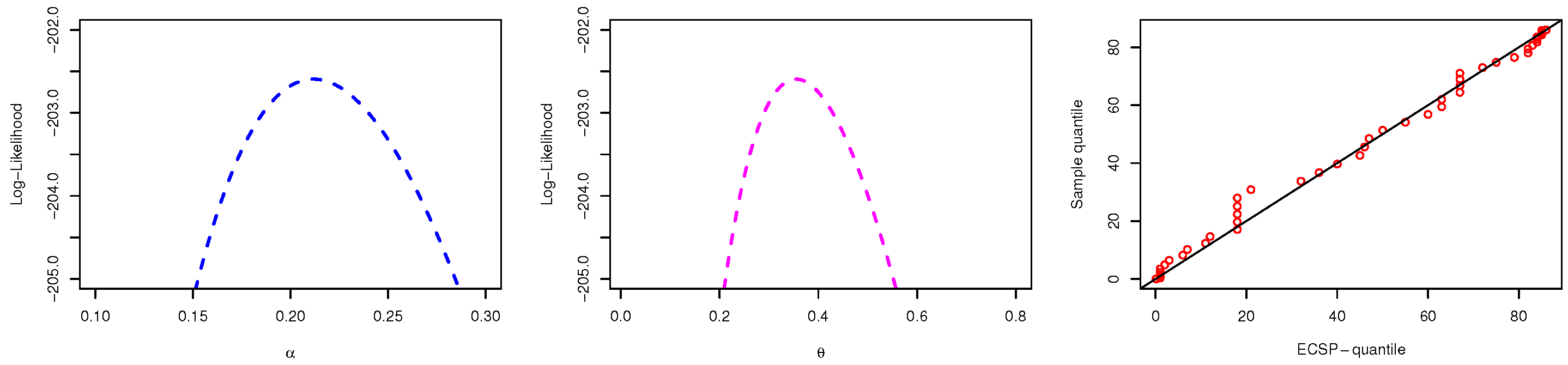
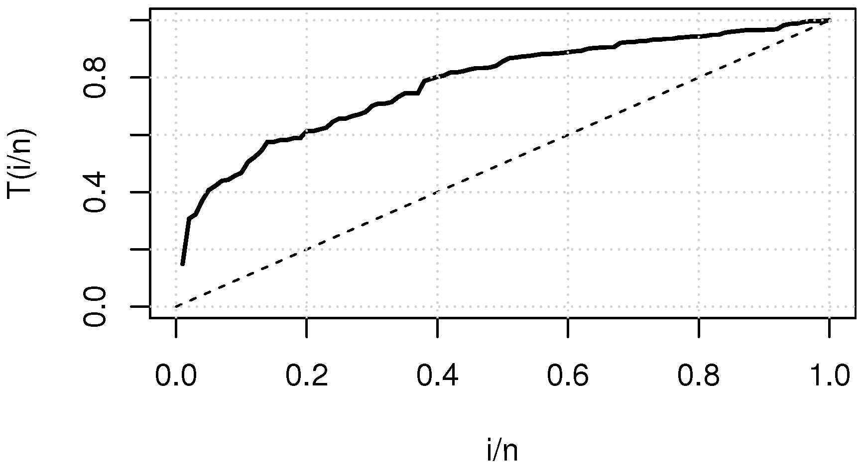
2.8.2. The ECSP Distribution
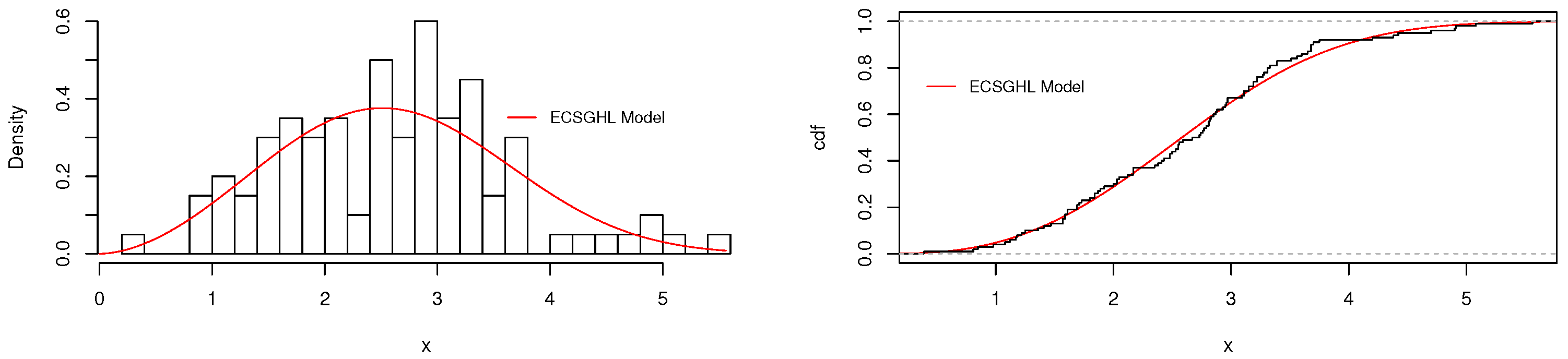
2.8.3. The ECSGHL Distribution
- As , the mean residual life of X satisfies:
- As , the mean reverse residual life of X satisfies:
- Let where and , then:for . The cdf of the standard Gumbel distribution was obtained as limit; converged in distribution to a random variable with such a Gumbel distribution.
- Let where and , then:for . The cdf of the W distribution of parameters 1 and θ was obtained as limit; converged in distribution to a random variable with such a W distribution.
3. Estimation
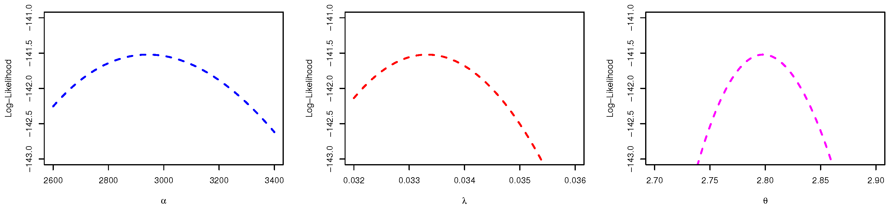
3.1. MLE
3.2. LSE
3.3. PE
3.4. BE
- Start by initial guess ;
- Set ;
- Use the Metropolis–Hastings algorithm to generate from ;
- Use the Metropolis–Hastings algorithm to generate from ;
- Set ;
- Repeat steps three to five, T times.
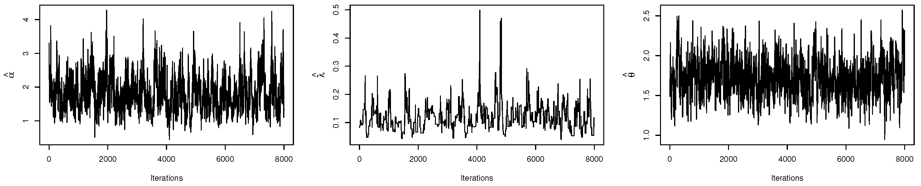
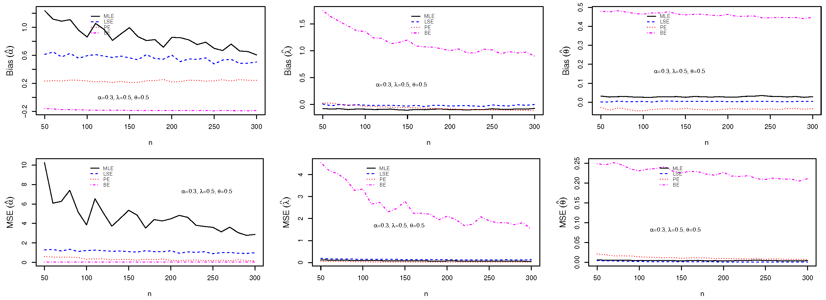
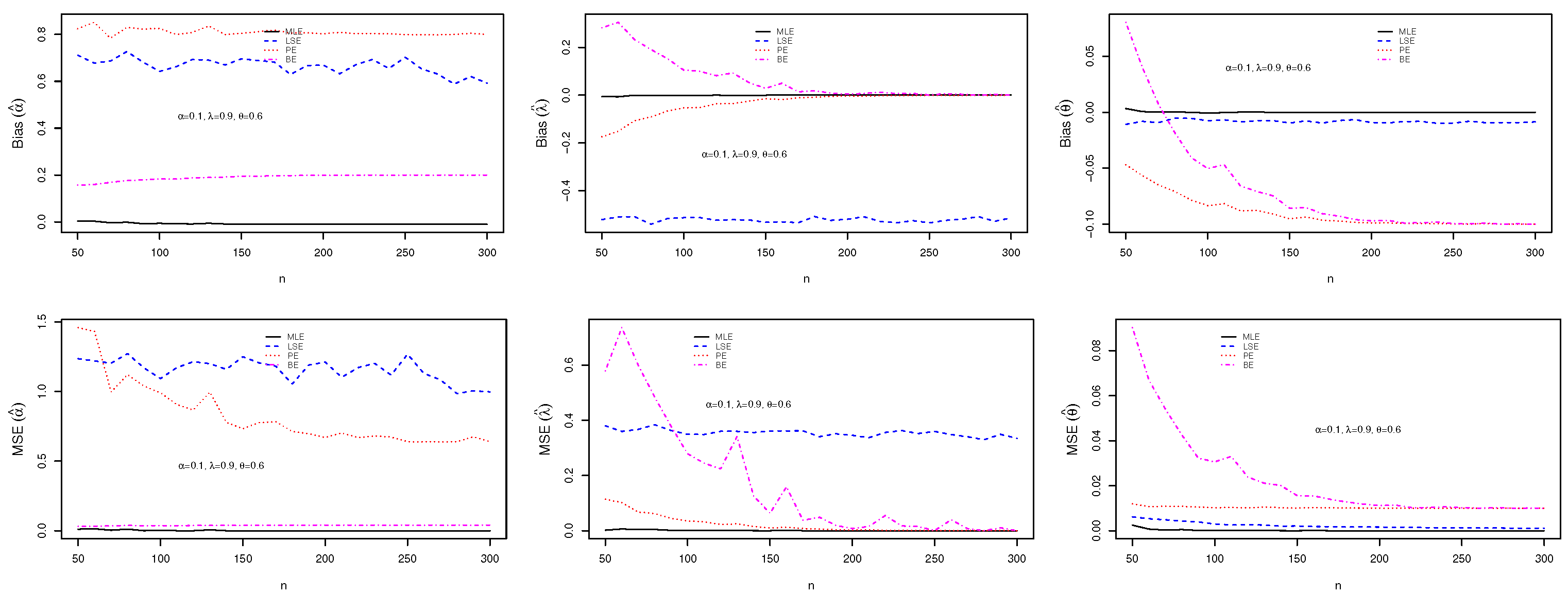
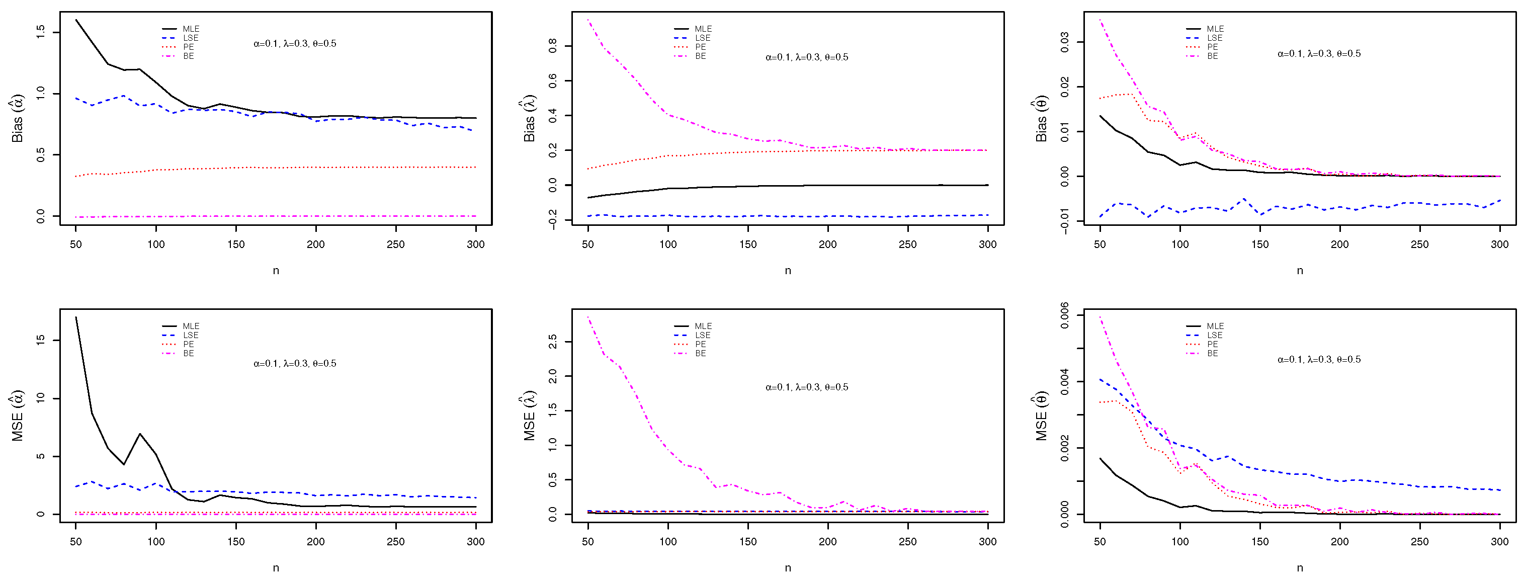
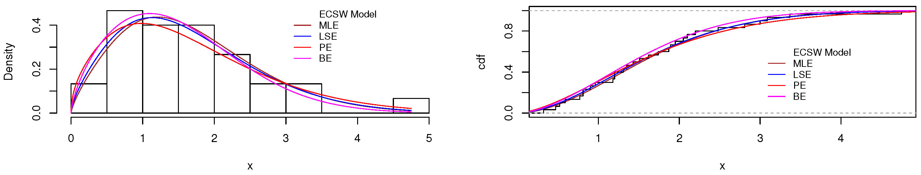
3.5. Simulation Studies and Practice of the ECSW Model
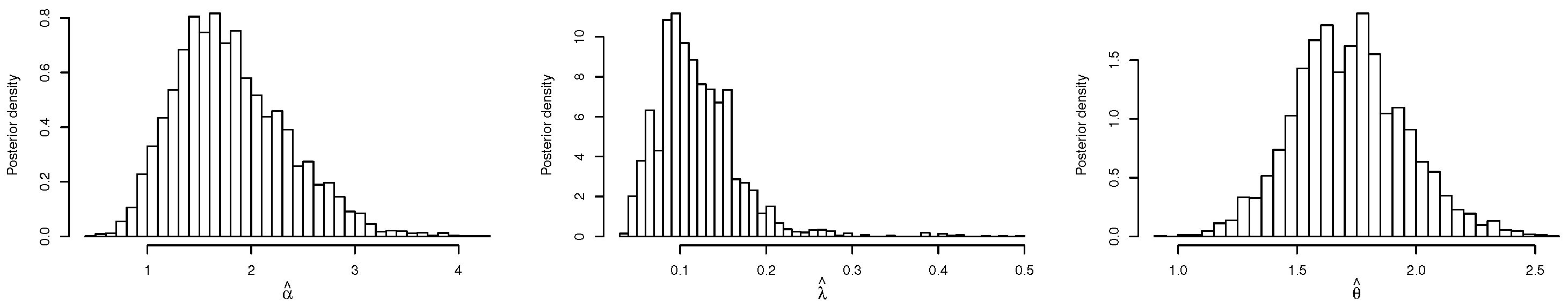
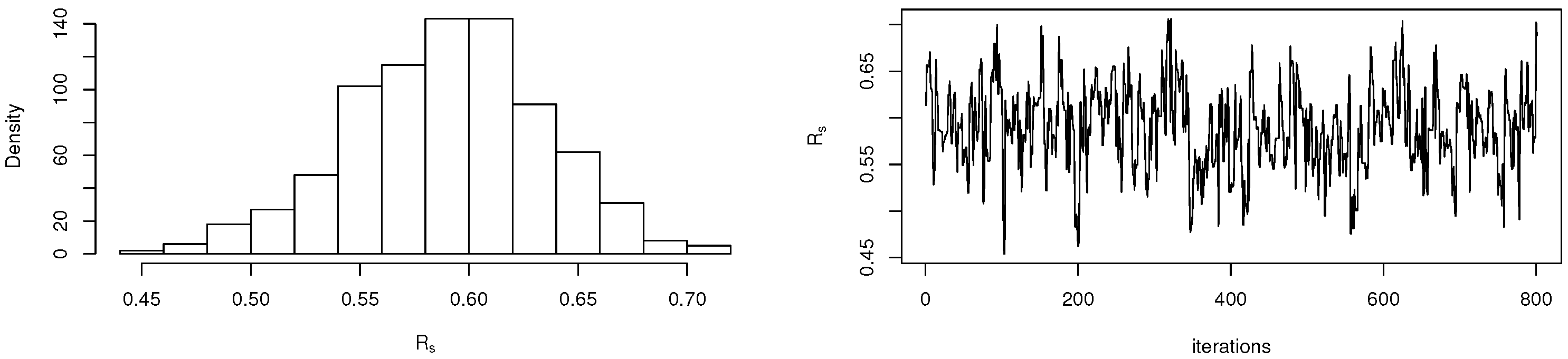
3.6. BE of the Reliability Parameter of the ECSW Distribution
3.7. Simulation Studies for the Reliability Parameter from the ECSW Distribution
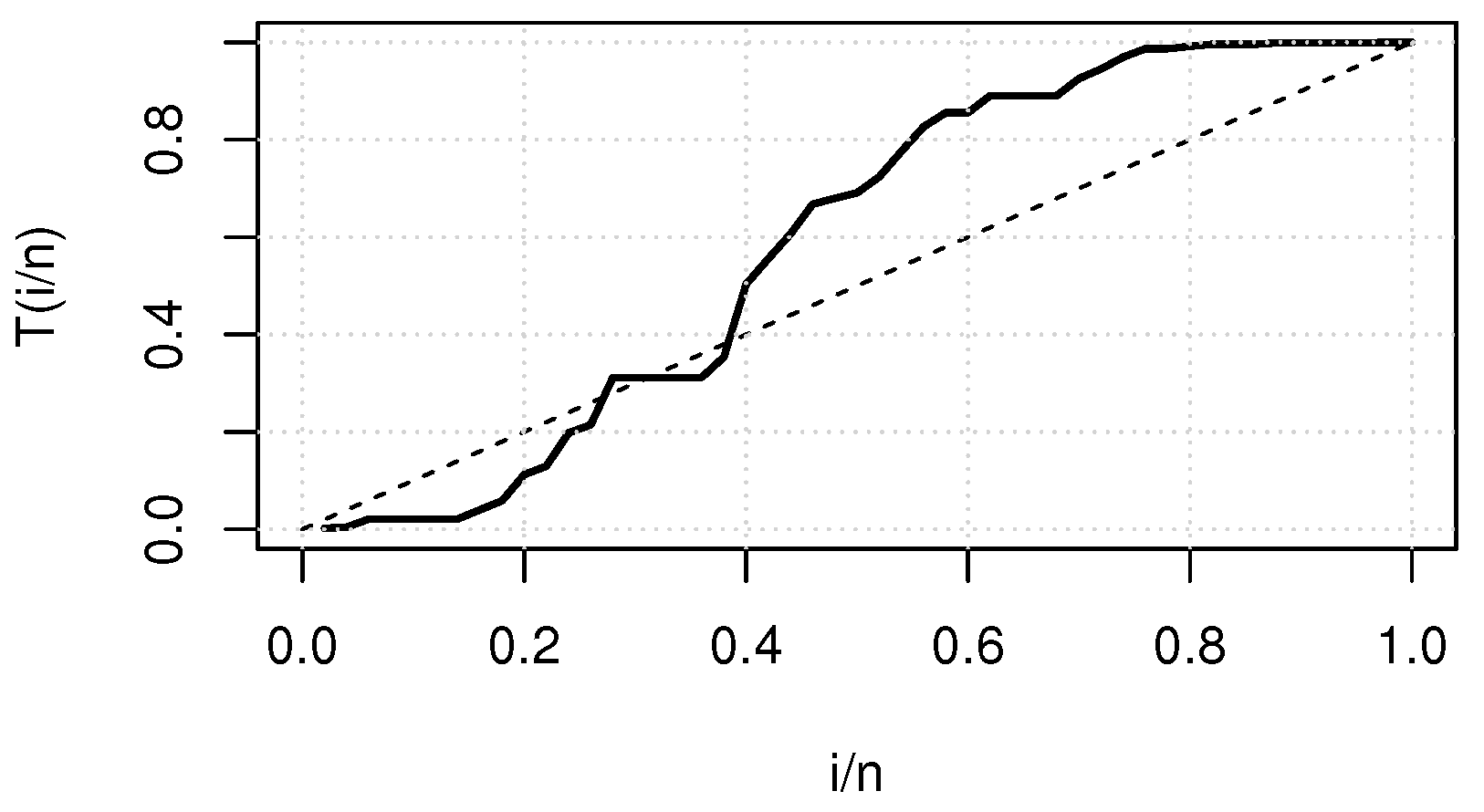
4. Real Data Illustration
4.1. Real Data I
4.2. Real Data II
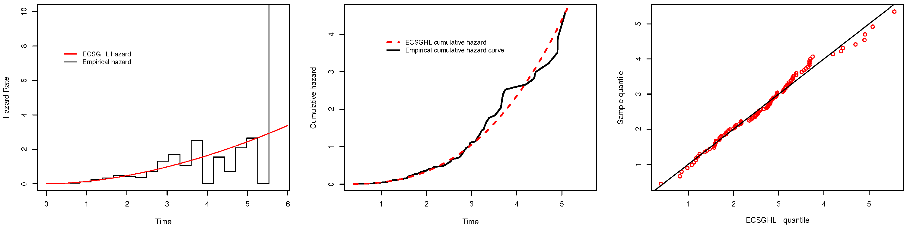
4.3. Real Data III
5. Conclusions
Author Contributions
Funding
Institutional Review Board Statement
Informed Consent Statement
Data Availability Statement
Acknowledgments
Conflicts of Interest
References
- Fisher, N.I. Statistical Analysis of Directional Data; University Press: Cambridge, UK, 1993. [Google Scholar]
- Evans, M.; Hastings, N.; Peacock, B. Statistical Distributions; IOP Publishing: Bristol, UK, 2001. [Google Scholar]
- Nadarajah, S.; Kotz, S. Beta trigonometric distributions. Port. Econ. J. 2006, 5, 207–224. [Google Scholar] [CrossRef]
- Kent, J.T.; Tyler, D.E. Maximum likelihood estimation for the wrapped Cauchy distribution. J. Appl. Stat. 1988, 15, 247–254. [Google Scholar] [CrossRef]
- Al-Faris, R.Q.; Khan, S. Sine square distribution: A new statistical model based on the sine function. J. Appl. Probab. Stat. 2008, 3, 163–173. [Google Scholar]
- Souza, L.; Junior, W.; de Brito, C.; Chesneau, C.; Ferreira, T.; Soares, L. On the Sin-G class of distributions: Theory, model and application. J. Math. Model. 2019, 7, 357–379. [Google Scholar]
- Kumar, D.; Singh, U.; Singh, S.K. A new distribution using sine function-its application to bladder cancer patients data. J. Stat. Appl. Probab. 2015, 4, 417. [Google Scholar]
- Souza, L.; Junior, W.; de Brito, C.; Chesneau, C.; Ferreira, T.; Soares, L. General properties for the Cos-G Class of Distributions with Applications. Eurasian Bull. Math. 2019, 2, 63–79. [Google Scholar]
- Chesneau, C.; Bakouch, H.S.; Hussain, T. A new class of probability distributions via cosine and sine functions with applications. Commun. Stat. Simul. Comput. 2019, 48, 2287–2300. [Google Scholar] [CrossRef]
- Jamal, F.; Chesneau, C.; Bouali, D.; Ul Hassan, M. Beyond the Sin-G family: The transformed Sin-G family. PLoS ONE 2021, 16, e0250790. [Google Scholar] [CrossRef]
- Mahmood, Z.; Chesneau, C.; Tahir, M. A new sine-G family of distributions: Properties and applications. Bull. Comput. Appl. Math. 2019, 7, 53–81. [Google Scholar]
- Souza, L.; Junior, W.; de Brito, C.; Chesneau, C.; Fernandes, R.; Ferreira, T. Tan-G class of trigonometric distributions and its applications. Cubo 2021, 23, 1–20. [Google Scholar] [CrossRef]
- Jamal, F.; Chesneau, C. A new family of polyno-expo-trigonometric distributions with applications. Infin. Dimens. Anal. Quantum Probab. Relat. Top. 2019, 22, 1950027. [Google Scholar] [CrossRef] [Green Version]
- Al-Babtain, A.A.; Elbatal, I.; Chesneau, C.; Elgarhy, M. Sine Topp-Leone-G family of distributions: Theory and applications. Open Phys. 2020, 18, 574–593. [Google Scholar] [CrossRef]
- Jamal, F.; Chesneau, C.; Aidi, K. The sine extended odd Fréchet-G family of distribution with applications to complete and censored data. Math. Slovaca 2021, 71, 961–982. [Google Scholar] [CrossRef]
- Bakouch, H.S.; Chesneau, C.; Leao, J. A new lifetime model with a periodic hazard rate and an application. J. Stat. Comput. Simul. 2018, 88, 2048–2065. [Google Scholar] [CrossRef]
- Abate, J.; Choudhury, G.L.; Lucantoni, D.M.; Whitt, W. Asymptotic analysis of tail probabilities based on the computation of moments. Ann. Appl. Probab. 1995, 5, 983–1007. [Google Scholar] [CrossRef]
- Gupta, R.C.; Gupta, P.L.; Gupta, R.D. Modeling failure time data by Lehman alternatives. Commun. Stat.-Theory Methods 1998, 27, 887–904. [Google Scholar] [CrossRef]
- Poondi, K. A generalized probability density function for double-bounded random processes. J. Hydrol. 1980, 46, 79–88. [Google Scholar]
- Gradshteyn, I.; Ryzhik, I.; Jeffrey, A.; Zwillinger, D. Table of Integrals, Series and Products, 7th ed.; Academic Press: New York, NY, USA, 2007. [Google Scholar]
- Kotz, S.; Pensky, M. The Stress-Strength Model and Its Generalizations: Theory and Applications; World Scientific: Singapore, 2003. [Google Scholar]
- Guo, H.; Krishnamoorthy, K. New approximate inferential methods for the reliability parameter in a stress–strength model: The normal case. Commun. Stat.-Theory Methods 2004, 33, 1715–1731. [Google Scholar] [CrossRef]
- Barbiero, A. Confidence intervals for reliability of stress-strength models in the normal case. Commun. Stat.-Simul. Comput. 2011, 40, 907–925. [Google Scholar] [CrossRef]
- Baklizi, A.; El-Masri, A.E.Q. Shrinkage estimation of P (X < Y) in the exponential case with common location parameter. Metrika 2004, 59, 163–171. [Google Scholar]
- Asgharzadeh, A.; Valiollahi, R.; Raqab, M.Z. Estimation of the stress—Strength reliability for the generalized logistic distribution. Stat. Methodol. 2013, 15, 73–94. [Google Scholar] [CrossRef]
- Krishnamoorthy, K.; Lin, Y. Confidence limits for stress—Strength reliability involving Weibull models. J. Stat. Plan. Inference 2010, 140, 1754–1764. [Google Scholar] [CrossRef]
- Kundu, D.; Gupta, R.D. Estimation of P [Y < X] for Weibull distributions. IEEE Trans. Reliab. 2006, 55, 270–280. [Google Scholar]
- Asgharzadeh, A.; Valiollahi, R.; Raqab, M.Z. Stress-strength reliability of Weibull distribution based on progressively censored samples. SORT-Stat. Oper. Res. Trans. 2011, 35, 103–124. [Google Scholar]
- Kundu, D.; Gupta, R.D. Estimation of P [Y < X] for generalized exponential distribution. Metrika 2005, 61, 291–308. [Google Scholar]
- Nadarajah, S.; Bagheri, S.; Alizadeh, M.; Samani, E.B. Estimation of the stress strength parameter for the generalized exponential-Poisson distribution. J. Test. Eval. 2018, 46, 2184–2202. [Google Scholar] [CrossRef]
- Shrahili, M.; Elbatal, I.; Muhammad, I.; Muhammad, M. Properties and applications of beta Erlang-truncated exponential distribution. J. Math. Comput. Sci. (JMCS) 2021, 22, 16–37. [Google Scholar] [CrossRef]
- Muhammad, M.; Liu, L. A New Extension of the Generalized Half Logistic Distribution with Applications to Real Data. Entropy 2019, 21, 339. [Google Scholar] [CrossRef] [Green Version]
- Muhammad, I.; Wang, X.; Li, C.; Yan, M.; Chang, M. Estimation of the Reliability of a Stress–Strength System from Poisson Half Logistic Distribution. Entropy 2020, 22, 1307. [Google Scholar] [CrossRef]
- Arnold, B.C.; Balakrishnan, N.; Nagaraja, H.N. A First Course in Order Statistics; Society for Industrial and Applied Mathematics: Philadelphia, PA, USA, 1992; Volume 54. [Google Scholar]
- Mächler, M. Arbitrarily Accurate Computation with R: The Rmpfr Package. Available online: https://cran.r-project.org/web/packages/Rmpfr/vignettes/Rmpfr-pkg.pdf (accessed on 1 October 2021).
- Kantam, R.; Ramakrishna, V.; Ravikumar, M. Estimation and testing in type I generalized half logistic distribution. J. Mod. Appl. Stat. Methods 2013, 12, 22. [Google Scholar] [CrossRef]
- Chen, M.H.; Shao, Q.M. Monte Carlo estimation of Bayesian credible and HPD intervals. J. Comput. Graph. Stat. 1999, 8, 69–92. [Google Scholar]
- Metropolis, N.; Rosenbluth, A.W.; Rosenbluth, M.N.; Teller, A.H.; Teller, E. Equation of state calculations by fast computing machines. J. Chem. Phys. 1953, 21, 1087–1092. [Google Scholar] [CrossRef] [Green Version]
- Hastings, W.K. Monte Carlo sampling methods using Markov chains and their applications. Biometrika 1970, 57, 97–109. [Google Scholar] [CrossRef]
- Gelfand, A.E.; Smith, A.F. Sampling-based approaches to calculating marginal densities. J. Am. Stat. Assoc. 1990, 85, 398–409. [Google Scholar] [CrossRef]
- Team, R.C. R: A Language and Environment for Statistical Computing; R Foundation for Statistical Computing: Vienna, Austria, 2019. [Google Scholar]
- Hinkley, D. On quick choice of power transformation. J. R. Stat. Soc. Ser. C (Appl. Stat.) 1977, 26, 67–69. [Google Scholar] [CrossRef]
- Seo, J.I.; Kang, S.B. Notes on the exponentiated half logistic distribution. Appl. Math. Model. 2015, 39, 6491–6500. [Google Scholar] [CrossRef]
- Bagheri, S.; Samani, E.B.; Ganjali, M. The generalized modified Weibull power series distribution: Theory and applications. Comput. Stat. Data Anal. 2016, 94, 136–160. [Google Scholar] [CrossRef]
- Muhammad, M. Poisson-odd generalized exponential family of distributions: Theory and applications. Hacet. J. Math. Stat. 2016, 47, 1652–1670. [Google Scholar] [CrossRef]
- Sarhan, A.M.; Abd EL-Baset, A.A.; Alasbahi, I.A. Exponentiated generalized linear exponential distribution. Appl. Math. Model. 2013, 37, 2838–2849. [Google Scholar] [CrossRef]
- Torabi, H.; Hedesh, N.M. The gamma-uniform distribution and its applications. Kybernetika 2012, 48, 16–30. [Google Scholar]
- Sarhan, A.M.; Kundu, D. Generalized linear failure rate distribution. Commun. Stat.-Theory Methods 2009, 38, 642–660. [Google Scholar] [CrossRef] [Green Version]
- Lee, C.; Famoye, F.; Olumolade, O. Beta-Weibull distribution: Some properties and applications to censored data. J. Mod. Appl. Stat. Methods 2007, 6, 17. [Google Scholar] [CrossRef]
- Carrasco, J.M.; Ortega, E.M.; Cordeiro, G.M. A generalized modified Weibull distribution for lifetime modeling. Comput. Stat. Data Anal. 2008, 53, 450–462. [Google Scholar] [CrossRef]
- Lai, C.; Xie, M.; Murthy, D. A modified Weibull distribution. IEEE Trans. Reliab. 2003, 52, 33–37. [Google Scholar] [CrossRef] [Green Version]
- Mahmoud, M.A.; Alam, F.M.A. The generalized linear exponential distribution. Stat. Probab. Lett. 2010, 80, 1005–1014. [Google Scholar] [CrossRef]
- Silva, G.O.; Ortega, E.M.; Cordeiro, G.M. The beta modified Weibull distribution. Lifetime Data Anal. 2010, 16, 409–430. [Google Scholar] [CrossRef]
- Cordeiro, G.M.; de Andrade, T.A.; Bourguignon, M.; Gomes-Silva, F. The exponentiated generalized standardized half-logistic distribution. Int. J. Stat. Probab. 2017, 6, 24–42. [Google Scholar] [CrossRef] [Green Version]
- Abdel-Hamid, A.H. Properties, estimations and predictions for a Poisson-half-logistic distribution based on progressively type-II censored samples. Appl. Math. Model. 2016, 40, 7164–7181. [Google Scholar] [CrossRef]
- Olapade, A. The type I generalized half logistic distribution. J. Iran. Stat. Soc. 2014, 13, 69–82. [Google Scholar]
- Jose, J.K.; Manoharan, M. Beta half logistic distribution—A new probability model for lifetime data. J. Stat. Manag. Syst. 2016, 19, 587–604. [Google Scholar] [CrossRef]
- Muhammad, M.; Yahaya, M.A. The half logistic-Poisson distribution. Asian J. Math. Appl. 2017, 2017. [Google Scholar]
- Muhammad, M. Generalized half-logistic Poisson distributions. Commun. Stat. Appl. Methods 2017, 24, 353–365. [Google Scholar] [CrossRef] [Green Version]
- Muhammad, M.; Liu, L. A New Three Parameter Lifetime Model: The Complementary Poisson Generalized Half Logistic Distribution. IEEE Access 2021, 9, 60089–60107. [Google Scholar] [CrossRef]
- Aarset, M.V. How to identify a bathtub hazard rate. IEEE Trans. Reliab. 1987, 36, 106–108. [Google Scholar] [CrossRef]
- Nichols, M.D.; Padgett, W. A bootstrap control chart for Weibull percentiles. Qual. Reliab. Eng. Int. 2006, 22, 141–151. [Google Scholar] [CrossRef]
- Bader, M.; Priest, A. Statistical aspects of fibre and bundle strength in hybrid composites. In Progress in Science and Engineering of Composites; NHPC: Edmonton, AB, Canada, 1982; pp. 1129–1136. [Google Scholar]
- Raqab, M.Z.; Madi, M.T.; Kundu, D. Estimation of P (Y < X) for the three-parameter generalized exponential distribution. Commun. Stat. Methods 2008, 37, 2854–2864. [Google Scholar]


| ECSW | KS | AD | CVM | |||
|---|---|---|---|---|---|---|
| MLE | 0.2182 | 0.8029 | 1.7340 | 0.0647 (0.9987) | 0.1522 (0.9545) | 0.0196 (0.9690) |
| LSE | 0.1992 | 0.9374 | 1.6669 | 0.0598 (0.9997) | 0.1429 (0.9668) | 0.0184 (0.9787) |
| PE | 0.2057 | 0.9962 | 1.4871 | 0.0838 (0.9727) | 0.1232 (0.9853) | 0.0157 (0.9914) |
| BE | 1.8027 | 0.1192 | 1.7202 | 0.0729 (0.9936) | 0.1889 (0.8928) | 0.0253 (0.9007) |
| (n, m) | ALCI | |||||||||||
|---|---|---|---|---|---|---|---|---|---|---|---|---|
| (1.0, 1.0, 1.0, 1.0, 1.0, 0.5000) | (20, 20) | 0.4995 | 0.0059 | 0.5008 | 0.0061 | 0.5028 | 0.0071 | 0.4751 | 0.0072 | 0.4925 | 0.0060 | 0.3186 |
| (−0.0005) | (0.0008) | (0.0023) | (−0.0249) | (−0.0075) | (0.96) | |||||||
| (30, 20) | 0.4613 | 0.0057 | 0.4619 | 0.0054 | 0.4624 | 0.0066 | 0.4394 | 0.0058 | 0.4554 | 0.0051 | 0.2907 | |
| (0.0082) | (0.0088) | (0.0094) | (−0.0137) | (0.0024) | (0.95) | |||||||
| (30, 40) | 0.5017 | 0.0035 | 0.5024 | 0.0036 | 0.5029 | 0.0044 | 0.4876 | 0.0039 | 0.4974 | 0.0035 | 0.2511 | |
| (0.0017) | (0.0024) | (0.0029) | (−0.0124) | (−0.0026) | (0.96) | |||||||
| (50, 40) | 0.4998 | 0.0029 | 0.5003 | 0.0030 | 0.5011 | 0.0034 | 0.4884 | 0.0032 | 0.4962 | 0.0029 | 0.2272 | |
| (−0.0002) | (0.0003) | (0.0011) | (−0.0116) | (−0.0037) | (0.96) | |||||||
| (60, 60) | 0.5018 | 0.0024 | 0.5021 | 0.0025 | 0.5027 | 0.0029 | 0.4935 | 0.0026 | 0.4991 | 0.0024 | 0.1964 | |
| (0.0018) | (0.0021) | (0.0027) | (−0.0066) | (−0.0009) | (0.95) | |||||||
| (2.0, 3.5, 0.9, 0.6, 2.0, 0.8396) | (20, 20) | 0.8302 | 0.0034 | 0.8371 | 0.0034 | 0.8493 | 0.0039 | 0.8226 | 0.0040 | 0.8264 | 0.0037 | 0.2213 |
| (−0.0094) | (−0.0025) | (0.0097) | (−0.0017) | (−0.0132) | (0.93) | |||||||
| (30, 20) | 0.8289 | 0.0030 | 0.8348 | 0.0030 | 0.8443 | 0.0034 | 0.8225 | 0.0035 | 0.8256 | 0.0032 | 0.2060 | |
| (−0.0107) | (−0.0048) | (0.0047) | (−0.0171) | (−0.0139) | (0.94) | |||||||
| (30, 40) | 0.8385 | 0.0022 | 0.8428 | 0.0023 | 0.8493 | 0.0026 | 0.8344 | 0.0024 | 0.8363 | 0.0023 | 0.1698 | |
| (−0.0011) | (0.0033) | (0.0097) | (−0.0052) | (−0.0032) | (0.91) | |||||||
| (50, 40) | 0.8359 | 0.0017 | 0.8392 | 0.0017 | 0.8452 | 0.0019 | 0.8326 | 0.0018 | 0.8341 | 0.0018 | 0.1526 | |
| (−0.0037) | (−0.0003) | (0.0056) | (−0.0069) | (−0.0054) | (0.93) | |||||||
| (60, 60) | 0.8404 | 0.0012 | 0.8429 | 0.0012 | 0.8469 | 0.0015 | 0.8381 | 0.0013 | 0.8392 | 0.0012 | 0.1307 | |
| (0.0008) | (0.0034) | (0.0074) | (−0.0015) | (−0.0004) | (0.93) | |||||||
| (1.3, 1.4, 0.5, 0.6, 0.5, 0.4995) | (20, 20) | 0.4970 | 0.0063 | 0.4985 | 0.0066 | 0.5009 | 0.0080 | 0.4704 | 0.0078 | 0.4891 | 0.0064 | 0.3261 |
| (−0.0025) | (−0.0009) | (0.0014) | (−0.0291) | (−0.0099) | (0.96) | |||||||
| (30, 20) | 0.5005 | 0.0059 | 0.5016 | 0.0062 | 0.5030 | 0.0074 | 0.4779 | 0.0068 | 0.4940 | 0.0059 | 0.3039 | |
| (0.0010) | (0.0021) | (0.0036) | (−0.0216) | (−0.0055) | (0.95) | |||||||
| (30, 40) | 0.4962 | 0.0044 | 0.4971 | 0.0045 | 0.4978 | 0.0054 | 0.4807 | 0.0049 | 0.4916 | 0.0044 | 0.2585 | |
| (−0.0032) | (−0.0024) | (−0.0016) | (−0.0188) | (−0.0079) | (0.95) | |||||||
| (50, 40) | 0.4959 | 0.0030 | 0.4964 | 0.0031 | 0.4967 | 0.0038 | 0.4838 | 0.0034 | 0.4922 | 0.0031 | 0.2317 | |
| (−0.0035) | (−0.0031) | (−0.0027) | (−0.0156) | (−0.0072) | (0.96) | |||||||
| (60, 60) | 0.4974 | 0.0024 | 0.4978 | 0.0024 | 0.4986 | 0.0029 | 0.4887 | 0.0026 | 0.4947 | 0.0024 | 0.1995 | |
| (−0.0020) | (−0.0017) | (−0.0009) | (−0.0108) | (−0.0048) | (0.96) | |||||||
| (1.3, 1.2, 1.5, 1.5, 1.5, 0.4800) | (20, 20) | 0.4873 | 0.0064 | 0.4883 | 0.0067 | 0.4890 | 0.0080 | 0.4609 | 0.0077 | 0.4800 | 0.0064 | 0.3265 |
| (0.0073) | (0.0084) | (0.0099) | (−0.0190) | (−0.0001) | (0.95) | |||||||
| (30, 20) | 0.4850 | 0.0062 | 0.4856 | 0.0064 | 0.4859 | 0.0075 | 0.4626 | 0.0072 | 0.4786 | 0.0062 | 0.3038 | |
| (0.0050) | (0.0056) | (0.0059) | (−0.0174) | (−0.0014) | (0.93) | |||||||
| (30, 40) | 0.4841 | 0.0042 | 0.4846 | 0.0044 | 0.4849 | 0.0053 | 0.4687 | 0.0047 | 0.4796 | 0.0043 | 0.2574 | |
| (0.0041) | (0.0045) | (0.0049) | (−0.0113) | (−0.0004) | (0.94) | |||||||
| (50, 40) | 0.4824 | 0.0032 | 0.4827 | 0.0033 | 0.4832 | 0.0038 | 0.4701 | 0.0035 | 0.4787 | 0.0032 | 0.2319 | |
| (0.0024) | (0.0027) | (0.0032) | (−0.0099) | (−0.0013) | (0.96) | |||||||
| (60, 60) | 0.4810 | 0.0024 | 0.4813 | 0.0025 | 0.4809 | 0.0029 | 0.4720 | 0.0026 | 0.4783 | 0.0025 | 0.2005 | |
| (0.0010) | (0.0013) | (0.0009) | (−0.0080) | (−0.0017) | (0.95) | |||||||
| (2.0, 3.0, 1.0, 1.0, 1.0, 0.6000) | (20, 20) | 0.5924 | 0.0077 | 0.5953 | 0.0080 | 0.6000 | 0.0095 | 0.5711 | 0.0094 | 0.5851 | 0.0080 | 0.3231 |
| (−0.0076) | (−0.0047) | (0.0001) | (−0.0289) | (−0.0149) | (0.93) | |||||||
| (30, 20) | 0.5941 | 0.0063 | 0.5966 | 0.0065 | 0.6016 | 0.0076 | 0.5766 | 0.0075 | 0.5880 | 0.0065 | 0.2974 | |
| (−0.0059) | (−0.0034) | (0.0016) | (−0.0234) | (−0.0120) | (0.93) | |||||||
| (30, 40) | 0.5955 | 0.0043 | 0.5975 | 0.0044 | 0.6009 | 0.0050 | 0.5830 | 0.0049 | 0.5909 | 0.0044 | 0.2557 | |
| (−0.0045) | (−0.0025) | (0.0009) | (−0.0169) | (−0.0091) | (0.94) | |||||||
| (50, 40) | 0.5970 | 0.0033 | 0.5986 | 0.0034 | 0.6006 | 0.0039 | 0.5875 | 0.0037 | 0.5935 | 0.0034 | 0.2268 | |
| (−0.0030) | (−0.0014) | (0.0006) | (−0.0125) | (−0.0065) | (0.95) | |||||||
| (60, 60) | 0.5948 | 0.0028 | 0.5960 | 0.0027 | 0.5975 | 0.0032 | 0.5877 | 0.0029 | 0.5921 | 0.0027 | 0.1977 | |
| (−0.0052) | (−0.0040) | (−0.0025) | (−0.0123) | (−0.0079) | (00.94) | |||||||
| (0.9, 0.8, 0.6, 0.7, 0.8, 0.4531) | (20, 20) | 0.4633 | 0.0059 | 0.4641 | 0.0062 | 0.4661 | 0.0078 | 0.4362 | 0.0066 | 0.4562 | 0.0056 | 0.3195 |
| (0.0102) | (0.0110) | (0.0131) | (−0.0169) | (0.0031) | (0.96) | |||||||
| (30, 20) | 0.4565 | 0.0045 | 0.4569 | 0.0047 | 0.4568 | 0.0057 | 0.4330 | 0.0053 | 0.4504 | 0.0045 | 0.2987 | |
| (0.0035) | (0.0039) | (0.0037) | (−0.0201) | (−0.0027) | (0.96) | |||||||
| (30, 40) | 0.4617 | 0.0036 | 0.4622 | 0.0038 | 0.4619 | 0.0045 | 0.4459 | 0.0039 | 0.4573 | 0.0036 | 0.2531 | |
| (0.0087) | (0.0091) | (0.0089) | (−0.0072) | (0.0043) | (0.96) | |||||||
| (50, 40) | 0.4542 | 0.0027 | 0.4541 | 0.0028 | 0.4543 | 0.0032 | 0.4416 | 0.0030 | 0.4507 | 0.0027 | 0.2267 | |
| (0.0012) | (0.0011) | (0.0012) | (−0.0114) | (−0.0024) | (0.97) | |||||||
| (60, 60) | 0.4579 | 0.0022 | 0.4580 | 0.0022 | 0.4579 | 0.0027 | 0.4488 | 0.0023 | 0.4553 | 0.0022 | 0.1952 | |
| (0.0049) | (0.0049) | (0.0048) | (−0.0042) | (0.0022) | (0.96) | |||||||
| (1.1, 1.5, 1.2, 1.3, 1.0, 0.5551) | (20, 20) | 0.5380 | 0.0067 | 0.5412 | 0.0068 | 0.5447 | 0.0079 | 0.5146 | 0.0089 | 0.5315 | 0.0070 | 0.3285 |
| (−0.0161) | (−0.0139) | (−0.0105) | (−0.0405) | (−0.0237) | (0.95) | |||||||
| (30, 20) | 0.5463 | 0.0060 | 0.5482 | 0.0062 | 0.5513 | 0.0071 | 0.5264 | 0.0074 | 0.5399 | 0.0062 | 0.3037 | |
| (−0.0089) | (−0.0069) | (−0.0039) | (−0.0289) | (−0.0153) | (0.94) | |||||||
| (30, 40) | 0.5422 | 0.0044 | 0.5435 | 0.0045 | 0.5455 | 0.0053 | 0.5281 | 0.0053 | 0.5376 | 0.0046 | 0.2598 | |
| (−0.0129) | (−0.0116) | (−0.0097) | (−0.0269) | (−0.0176) | (0.94) | |||||||
| (50, 40) | 0.5477 | 0.0032 | 0.5488 | 0.0033 | 0.5501 | 0.0038 | 0.5369 | 0.0037 | 0.5441 | 0.0033 | 0.2311 | |
| (−0.0074) | (−0.0063) | (−0.0050) | (−0.0183) | (−0.0111) | (0.95) | |||||||
| (60, 60) | 0.5478 | 0.0026 | 0.5487 | 0.0026 | 0.5496 | 0.0030 | 0.5399 | 0.0029 | 0.5451 | 0.0026 | 0.2004 | |
| (−0.0072) | (−0.0064) | (−0.0054) | (−0.0152) | (−0.0100) | (0.96) |
| Distributions | L | AIC | CAIC | BIC | KS (p-Value) | |||||||
|---|---|---|---|---|---|---|---|---|---|---|---|---|
| ECSP | − | − | − | − | ||||||||
| GU | − | 86.713 | − | − | ||||||||
| TUq | − | − | − | |||||||||
| BMW | − | 0.165 | − | |||||||||
| BW | − | − | 0.070 | − | ||||||||
| MW | − | − | - | − | ||||||||
| EGLE | − | − | − | |||||||||
| GLE | − | − | − | − | ||||||||
| GLFR | − | − | − | − | ||||||||
| POGE-U | − | − | − | |||||||||
| GMWP | − | - | ||||||||||
| GMWL | − | - | ||||||||||
| GMWG | − | - | ||||||||||
| GMW | − | - | − | |||||||||
| P | − | − | − | − | − | 0.9999 () |
| Distributions | L | AIC | CAIC | BIC | KS | AD | CVM | ||||||
|---|---|---|---|---|---|---|---|---|---|---|---|---|---|
| ECSGHL | - | − | − | ||||||||||
| GHL | − | − | − | − | |||||||||
| PHL | − | − | − | − | |||||||||
| EGSHL | − | − | − | − | |||||||||
| CPGHL | − | − | − | ||||||||||
| BHL | − | − | − | ||||||||||
| HLP | − | − | − | − | 0.3202 (2.5e-9) | ||||||||
| OHL | − | − | − | − | 0.2778 (3.9e-7) |
Publisher’s Note: MDPI stays neutral with regard to jurisdictional claims in published maps and institutional affiliations. |
© 2021 by the authors. Licensee MDPI, Basel, Switzerland. This article is an open access article distributed under the terms and conditions of the Creative Commons Attribution (CC BY) license (https://creativecommons.org/licenses/by/4.0/).
Share and Cite
Muhammad, M.; Bantan, R.A.R.; Liu, L.; Chesneau, C.; Tahir, M.H.; Jamal, F.; Elgarhy, M. A New Extended Cosine—G Distributions for Lifetime Studies. Mathematics 2021, 9, 2758. https://doi.org/10.3390/math9212758
Muhammad M, Bantan RAR, Liu L, Chesneau C, Tahir MH, Jamal F, Elgarhy M. A New Extended Cosine—G Distributions for Lifetime Studies. Mathematics. 2021; 9(21):2758. https://doi.org/10.3390/math9212758
Chicago/Turabian StyleMuhammad, Mustapha, Rashad A. R. Bantan, Lixia Liu, Christophe Chesneau, Muhammad H. Tahir, Farrukh Jamal, and Mohammed Elgarhy. 2021. "A New Extended Cosine—G Distributions for Lifetime Studies" Mathematics 9, no. 21: 2758. https://doi.org/10.3390/math9212758
APA StyleMuhammad, M., Bantan, R. A. R., Liu, L., Chesneau, C., Tahir, M. H., Jamal, F., & Elgarhy, M. (2021). A New Extended Cosine—G Distributions for Lifetime Studies. Mathematics, 9(21), 2758. https://doi.org/10.3390/math9212758