Space: The Re-Visioning Frontier of Biological Image Analysis with Graph Theory, Computational Geometry, and Spatial Statistics

Abstract

Every biological image contains quantitative data that can be used to test hypotheses about how patterns were formed, what entities are associated with one another, and whether standard mathematical methods inform our understanding of biological phenomena. In particular, spatial point distributions and polygonal tessellations are particularly amendable to analysis with a variety of graph theoretic, computational geometric, and spatial statistical tools such as: Voronoi polygons; Delaunay triangulations; perpendicular bisectors; circumcenters; convex hulls; minimal spanning trees; Ulam trees; Pitteway violations; circularity; Clark-Evans spatial statistics; variance to mean ratios; Gabriel graphs; and, minimal spanning trees. Furthermore, biologists have developed a number of empirically related correlations for polygonal tessellations such as: Lewis’s law (the number of edges of convex polygons are positively correlated with the areas of these polygons): Desch’s Law (the number of edges of convex polygons are positively correlated with the perimeters of these polygons); and Errara’s Law (daughter cell areas should be roughly half that of their parent cells’ areas). We introduce a new Pitteway Law that the number of sides of the convex polygons in a Voronoi tessellation of biological epithelia is proportional to the minimal interior angle of the convex polygons as angles less than 90 degrees result in Pitteway violations of the Delaunay dual of the Voronoi tessellation.

1. Introduction

Visual representations can be used to test hypotheses, help us reason about biological causation, and help us communicate our inferences. While calculus and differential equations currently dominate applications of mathematics to biology, biologists are deeply interested in a wide variety of patterns in multiple forms of visualization and the causal mechanisms that generate such patterns. Unfortunately, visual areas of mathematics such as geometry and topology are rarely learned by biologists. Therefore, while we cannot make the case as in Star Trek that space is the final frontier, mathematical and computational analysis of space should allow us to re-vision biological image analysis by seriously applying graph theory, computational geometry, and spatial statistics. Recent articles in Σ Mathematics have described the importance of graph theory in biology: RNA structural motifs in viruses [1]; 3D icosahedra [2]; and non-Mendelian genetics [3]. While these articles address important mathematical concepts, they do not discuss the general utility of graph theory to biological problems. Graph theory relates especially well to this Special Issue on “mathematical biology” because biologists already use graphs such as phylogenetic trees, fate maps, pedigrees, chromosomal maps, food webs, connectomes, neural nets, and secondary structures of RNA (planar graphs such as Nussinov circles, domes, mountains, and airports) and proteins (HP (hydrophobic-polar) protein lattices; Wenxiang diagrams). These visualizations are mathematical abstractions of many biological phenomena. Nonetheless most biologists do not appreciate that these visualizations are amenable to analysis with formal mathematical tools. Particularly, visualizations such as photographs of tree canopies, fish territories on sandy or muddy bottom lakes, polygonal animal coat patterns, histological preparations of epithelial cell layers, radiolarians tests, viral capsids, or x-ray crystallographic images of protein structures lend themselves to analysis by tessellations of Voronoi polygons and their topological duals: Delaunay triangulations. Herein the mathematical power of these geometric and topological tools as well as a series of related concepts from graph theory, computational geometry, and spatial statistics will be explored in the context of image analysis of biological patterns.

2. Valuing Voronoi Visualization: Spatial Analysis of Biological Patterns of Points, Polygons, and Polytopes

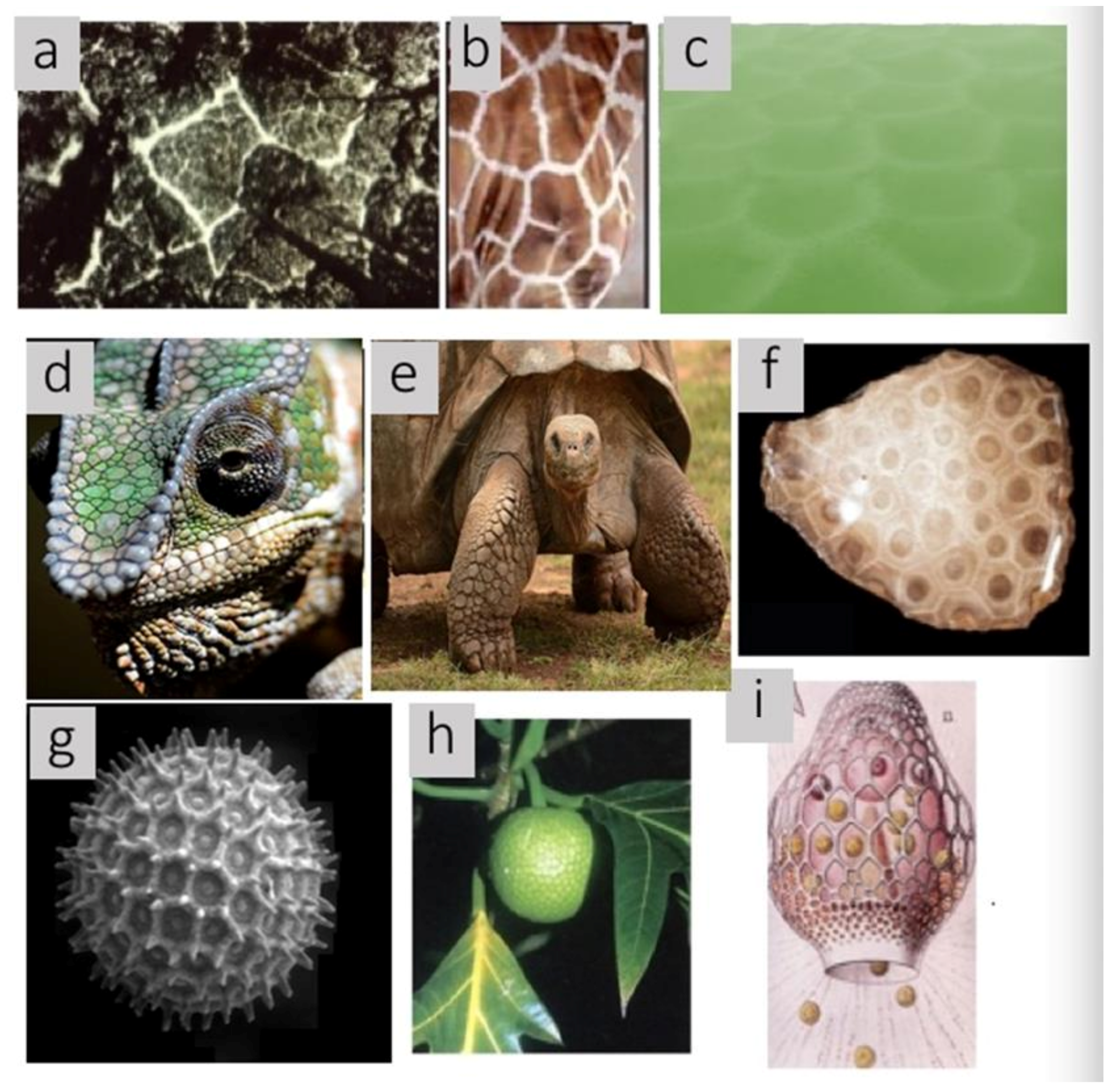
What do these biological tessellations share in common? Do these organic forms look quasi-crystalline? Do you see a preponderance of five- and six-sided convex polygons that primarily adjoin one another to form trigonal junctions? Why should such similar patterns occur across such vast scales of size, time, phylogeny, and causal mechanism? How can our appreciation of a very different use of standard geometry and algebra tools as well a little help from graph theory and spatial statistics help us to better understand the evolution, development, and beauty of biological patterns?

Allometry and fractals have captured the imagination of mathematical biologists as well as amateurs because both apply across at least ten orders of magnitude of biological phenomena and structures from the molecular to the ecological level. All of the biological specimens illustrated in Figure 1 contain tessellations of convex polygons known as Voronoi polygons. Voronoi polygons and polyhedra are less well known to both audiences, but scale equally well across phylogenetic, spatial, and temporal dimensions. Furthermore, Voronoi polygons and polyhedra are associated with additional mathematical methods that allow deeper insight into a variety of biological causal mechanisms such as growth, diffusion, division, packing, docking of ligands, strength of materials, molecular folding, foraging behavior, predator avoidance, and crowding as well as to their utility in making measurements, modeling interactions, relationship of two- and three-dimensional topographic structures, making succinct abstractions, and visualization per se. These four criteria of diversity:

(1)

Phylogenetic;

(2)

Spatial;

(3)

Temporal;

(4)

Causal mechanisms are posited as useful gauges of the applicability of mathematics and computer science to biology.

Lest we forget, mathematicians are deeply interested in biological pattern formation and morphogenesis in general. With the strong visual legacy of mathematical research in geometry, topology, and symmetry, McCormick, DeFanti, and Brown [4] state: “Visualization is a method of computing. It transforms the symbolic into the geometric, enabling researchers to observe their simulations and computations. Visualization offers a method for seeing the unseen. It enriches the process of scientific discovery and fosters profound and unexpected insights. In many fields it is already revolutionizing the way scientists do science.” It is precisely this desire to use mathematics to “see the unseen” that as a mathematical biologist I want to share with biologists. Gilbert [5] argues that mathematical visualization is a metacognitive skill that if students are able to acquire translates to many different problem-solving applications. Therefore, this is not simply a matter of interpreting pretty pictures, but a tool in helping both students and researchers to make deeper inferences about what they see.

Aurenhammer [6] has raised two questions and his answers are well worth noting: Why do Voronoi diagrams receive so much attention? What is special about this easily defined and visualized construct? It seems three main reasons are responsible.

First (science), Voronoi diagrams arise in nature in various situations. Indeed, several natural processes can be used to define particular classes of Voronoi diagrams. Human intuition is often guided by visual perception. If one sees an underlying structure, the whole situation may be understood at a higher level.

Second (mathematics), Voronoi diagrams have interesting and surprising mathematical properties; for instance, they are related to many well-known geometric structures. This has led several authors to believe that the Voronoi diagram is one of the most fundamental constructs defined by a discrete set of points.

Finally (computer science), Voronoi diagrams have proved to be a powerful tool in solving seemingly unrelated computational problems and therefore have increasingly attracted the attention of computer scientists in the last few years. Efficient and reasonably simple techniques have been developed for the construction and representation of Voronoi diagrams.

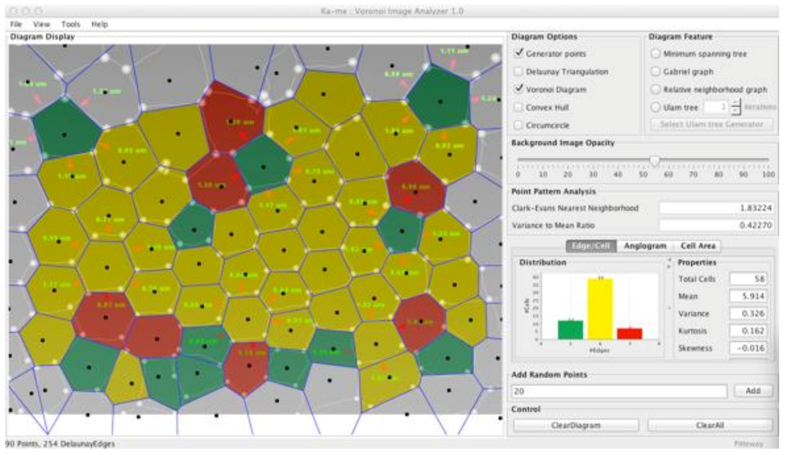
These considerations were fundamental driving forces in the development of our software: Ka-me: A Voronoi Visualizer [7]. However, the original motivation to develop such a tool began in 1977 with the use of Voronoi tessellations in cell biology by Hsiao Honda [8] and has been used by one of the authors in cellular and developmental biology courses ever since as well as in BioQUEST Curriculum Consortium workshops [fff]. Honda fundamentally addressed the question of whether Voronoi tessellations fit the number, size, and shape of single cell sheets of biological cells such as exist in epithelia and monolayers of cells grown on 2D surfaces in tissue culture. In an additional paper [ggg], he extended his analyses to dynamic rather than just static patterns. Thus, the breadth of spatial problems in biological image analysis will be explored throughout this paper and the power of Ka-me: A Voronoi Image Analyzer will elaborated for multiple kinds of biological images and to make inferences about the causal reasons for such patterns to exist.

2.1. Spatial Distributions

Voronoi tessellations abound in biological, medical, and environmental images across broad phylogenetic (Figure 1), spatial and temporal scales (

Table 1. Spatial diversity in biological formation of Voronoi patterns.

Size	Biological Pattern
1 kilometer	Aerial photograph of old human settlements
100 meters	“Canopy Puzzle”: Mature tropical rainforest
10 meters	Reticulated giraffe, Tilapia fish territories
1 meter	Galapagos tortoise, reticulated eel, leopard coat
1 decimeter	Petoskey stone (fossilized “stony coral), Thai breadfruit
1 centimeter	Slime mold, fish eggs packed
1 millimeter	Pollen grain, elytron of a beetle, leaf cross-section
100 microns	Radiolarian, cells in tissue culture
10 microns	Bacterial biofilm

; [8]) and are caused by a large variety of different mechanisms (Table 1). These tessellations have current interest for biologists because they are self-organizing, can cover an area in an efficiently constructed fashion with minimal lightweight material and extraordinarily strong structural properties, are natural instruments for evaluating measurement of nearest neighbor interactions, etc. They were formally characterized by the Ukrainian mathematician Georgii Feodosevich Voronoi in 1908 [9]. Further, many disciplines have rediscovered them and given them different names such as Wigner-Steitz cells in physics, Theissen polygons in geology, archaeology, and meteorology, Dirichlet domains in crystallography, and S-mosiacs in ecology. Recently, Gibson et al. [10,11] referred to Voronoi tessellations as “polygonal lattices.” Priority is usually given to Voronoi and will be adopted throughout this paper.

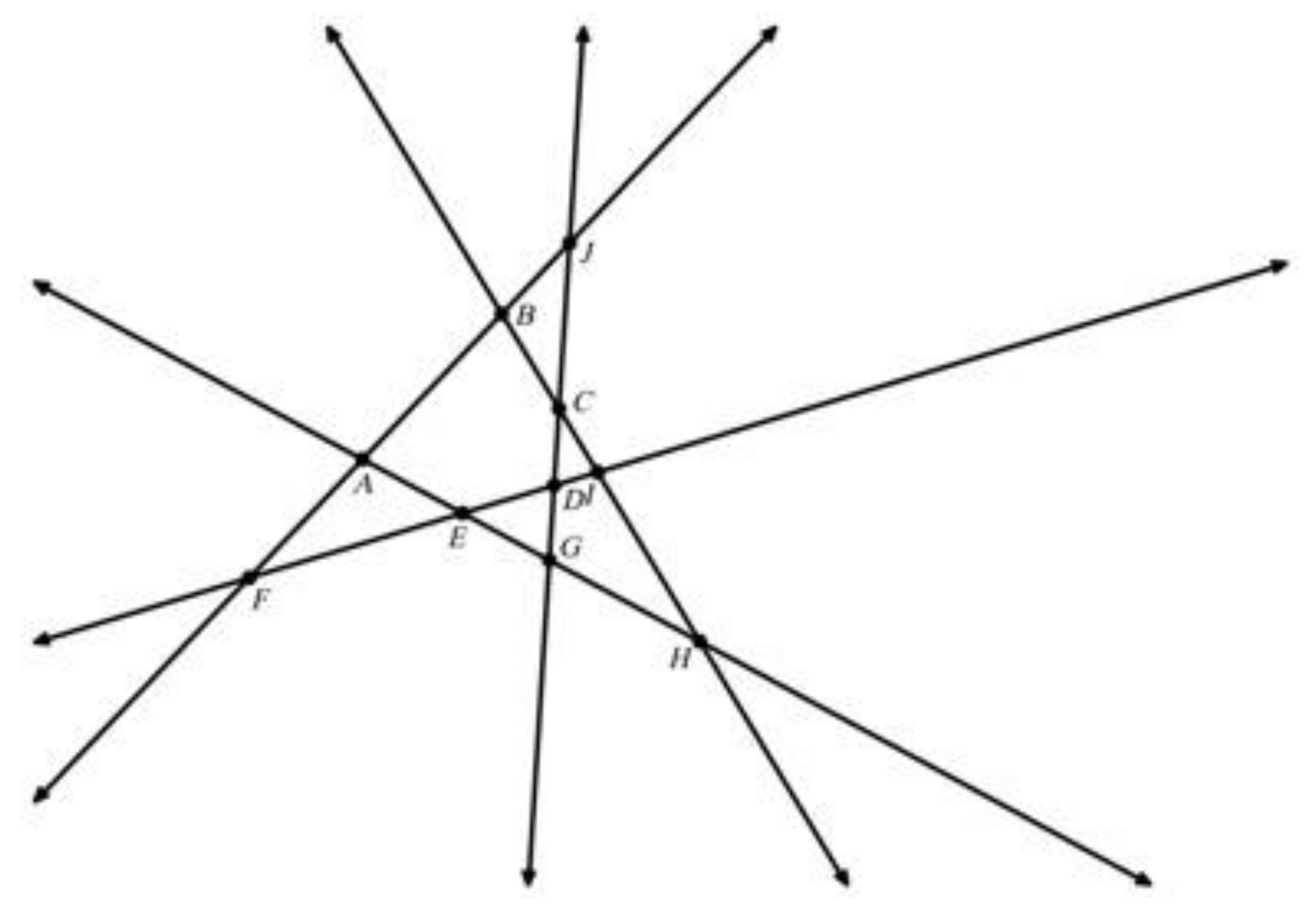
In order to test whether a particular biological pattern was actually a Voronoi tessellation, we tried to fit a Voronoi tessellation to the test of a radiolarian that we examined by 3D nanotomography [12] (see Figure 2). We converted the test of the radiolarian with a medial axial transformation with the software Amira [13] in order to obtain a flattened screen projection. Note that all 40 convex polygons on the surface fit quite well. On only a few cells out of the 40 fit inside of a convex hull (because polygons outside of this region extend to infinity) can you see the white lines of the underlying Amira image different from the edge of the fit Voronoi face and all 40 convex polygons have the same number of edges as their counterparts and cover nearly identical areas. Thus, to a good approximation, we can make the mathematical inference that whatever mechanism produced the pattern on the radiolarian test that there was a spatial point distribution of generator sources, and the edges are the perpendicular bisectors between these generators. In other words, the properties of Voronoi diagrams, namely that they produce tessellations with trigonal junctions equidistant from three neighboring generator points (that is, these trigonal junctions are the circumcenter of a circle that goes through all three neighboring generator points and the radius of the circle is the distance from each neighboring generator point and the circumcenter). Furthermore, anytime we see a polygonal tessellation which has a predominance of five and six sided convex polygons, it is likely to be the product of nearest neighbor (i.e., local interactions). Conversely, if we see a polygonal tessellation which has a predominance of three- and four-sided convex polygons with degree four junctions, it is likely to be the product of line-line intersections (i.e., long range interactions) (see Figure 3).

Equations for the circumcenter of a circle defined by three generator points x₁, y₁; x₂, y₂; and x₃, y₃.

$$y_c=\frac{\left[\left(x_3^2-x_2^2\right)+\left(y_3^2-y_2^2\right)\right]\left(x_1-x_2\right)+\left(x_2-x_3\right)\left[\left(y_1^2-y_2^2\right)+\left(x_1^2-x_2^2\right)\right]}{2\left(x_1-x_2\right)\left(y_3-y_2\right)+2\left(x_3-x_2\right)\left(y_2-y_1\right)}$$

and

$$x_c=\frac{\left(y_1^2-y_2^2\right)+\left(x_1^2-x_2^2\right)+2\left(y_2^2-y_1^2\right)y_c}{2\left(x_1-x_2\right)}$$

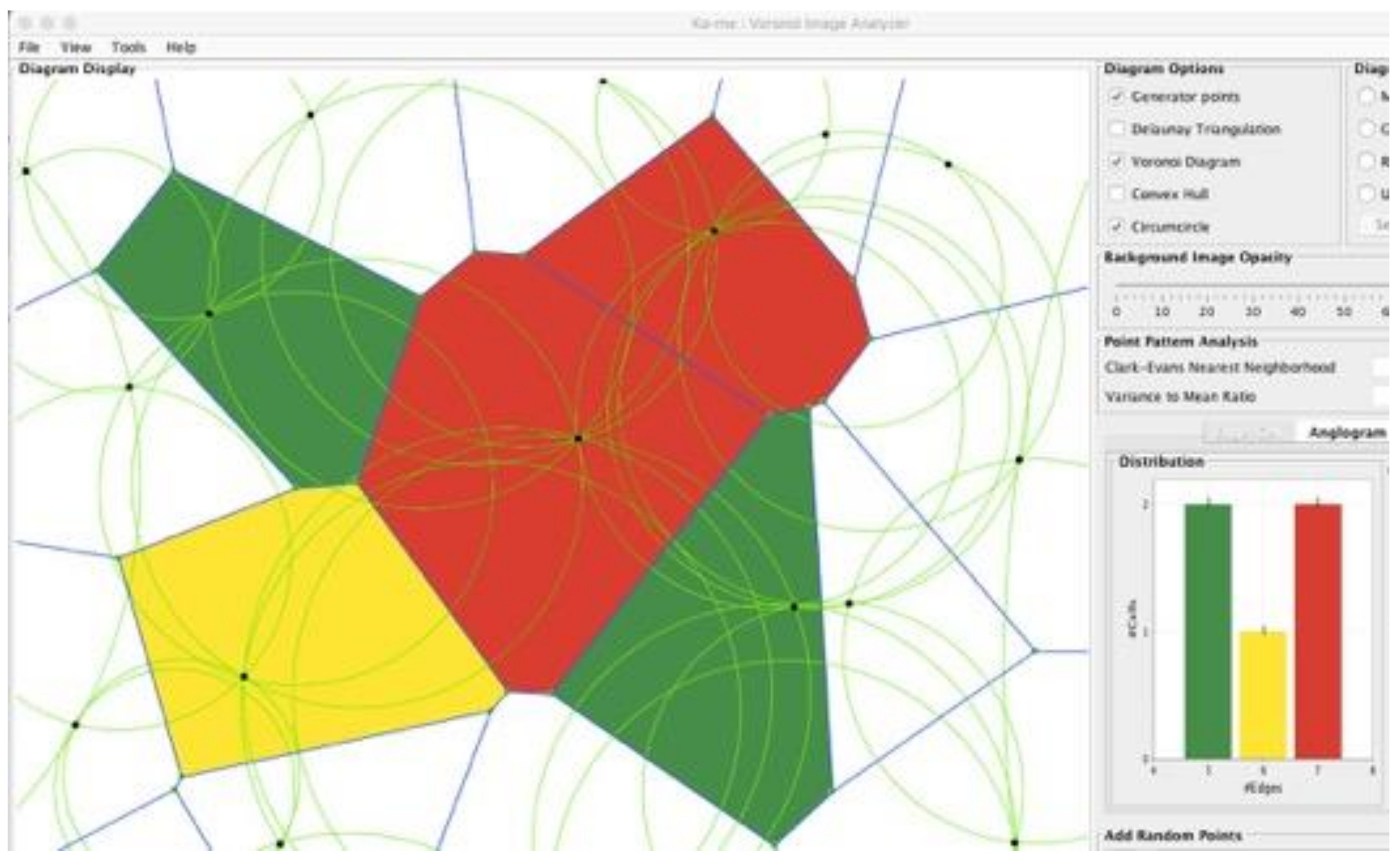
Then, by substitution of the coordinates of these two equations back into the original three equations, the length of the radius of the circumcircle can be determined. These circumcenters define a circle with all three generator points lying on it. Such circles are often referred to in the computational geometry field as the “greatest open circles.” For their construction see: https://www.youtube.com/watch?v=YBiAabFcPCI (accessed on 25 October 2021). Circumcircles are shown in a Ka-me analysis in Figure 4. The utility of these constructions is important to identify where you might locate a cell tower to improve phone coverage, add a rain-gauge, place a fire station or neighborhood school, or identify an area of least competition between animals of the same species. Each of these objects: the generator points, the Voronoi boundaries (perpendicular bisectors between the generator points), the vertices of the Voronoi polygons (circumcenters), the Delaunay triangulations, and the greatest open circles have different applications for different biological problems to which we will refer later.

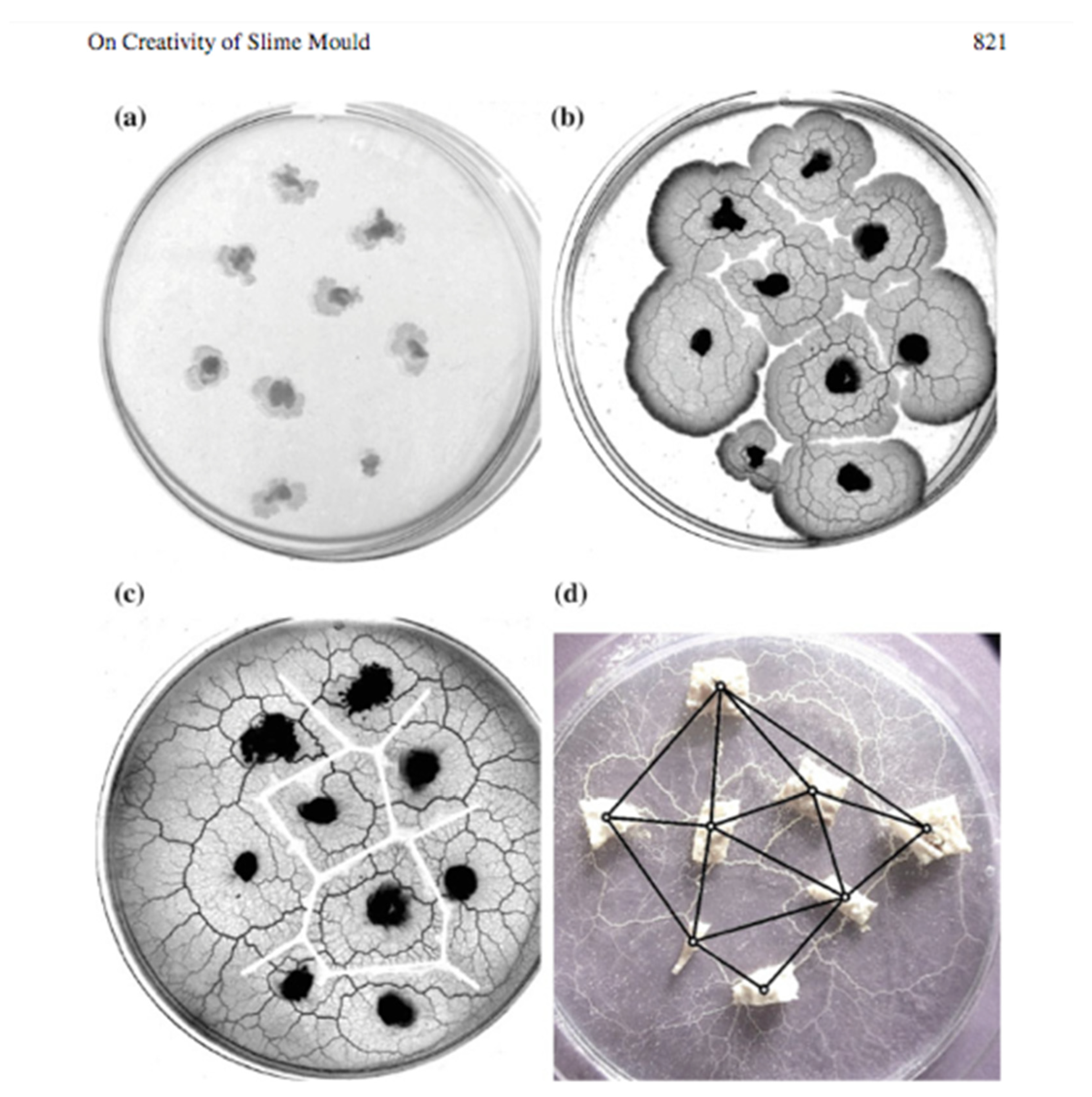
An interesting experimental demonstration (Figure 5) of a biological system capable of computing a Voronoi tessellation is given by Jones and Adamatzsky [14]: “Slime mould Physarum polycephalum is a large single cell capable for distributed sensing, concurrent information processing, parallel computation and decentralised actuation. The ease of culturing and experimenting with Physarum makes this slime mould an ideal substrate for real-world implementations of unconventional sensing and computing devices. In the last decade, the Physarum became a Swiss knife of the unconventional computing: give the slime mould a problem it will solve it. We provide a concise summary of what exact computing and sensing operations are implemented with live slime mould. The Physarum devices discussed range from morphological processors for computational geometry to experimental archeology tools, from self-routing wires to memristors, from devices approximating the shortest path to analog physical models of space exploration. Plasmodium growing on a nutrient substrate from a single site of inoculation expands circularly as a typical diffusive or excitation wave. When two plasmodium waves encounter each other, they stop propagating. To approximate a Voronoi diagram with Physarum, we physically map a configuration of planar data points by inoculating plasmodia on a substrate. Plasmodium waves propagate circularly from each data point and stop when they collide with each other. Thus, the plasmodium waves approximate a Voronoi diagram, whose edges are the substrate’s loci not occupied by plasmodia. Time complexity of the Physarum computation is proportional to a maximal distance between two geographically neighbouring data points, which is capped by a diameter of the data planar set, and does not depend on a number of the data points.

Shirakawa [15] goes one step further by simultaneously constructing both a Voronoi diagram and a Delaunay triangulation by Physarum Polycephalum. “We experimentally demonstrate that both Voronoi diagram and its dual graph Delaunay triangulation are simultaneously constructed—for specific conditions—in cultures of plasmodium, a vegetative state of Physarum polycephalum. Every point of a given planar data set is represented by a tiny mass of plasmodium. The plasmodia spread from their initial locations but, in certain conditions, stop spreading when they encounter plasmodia originated from different locations. Thus, space loci not occupied by the plasmodia represent edges of Voronoi diagram of the given planar set. At the same time, the plasmodia originating at neighboring locations form merging protoplasmic tubes, where the strongest tubes approximate Delaunay triangulation of the given planar set.”

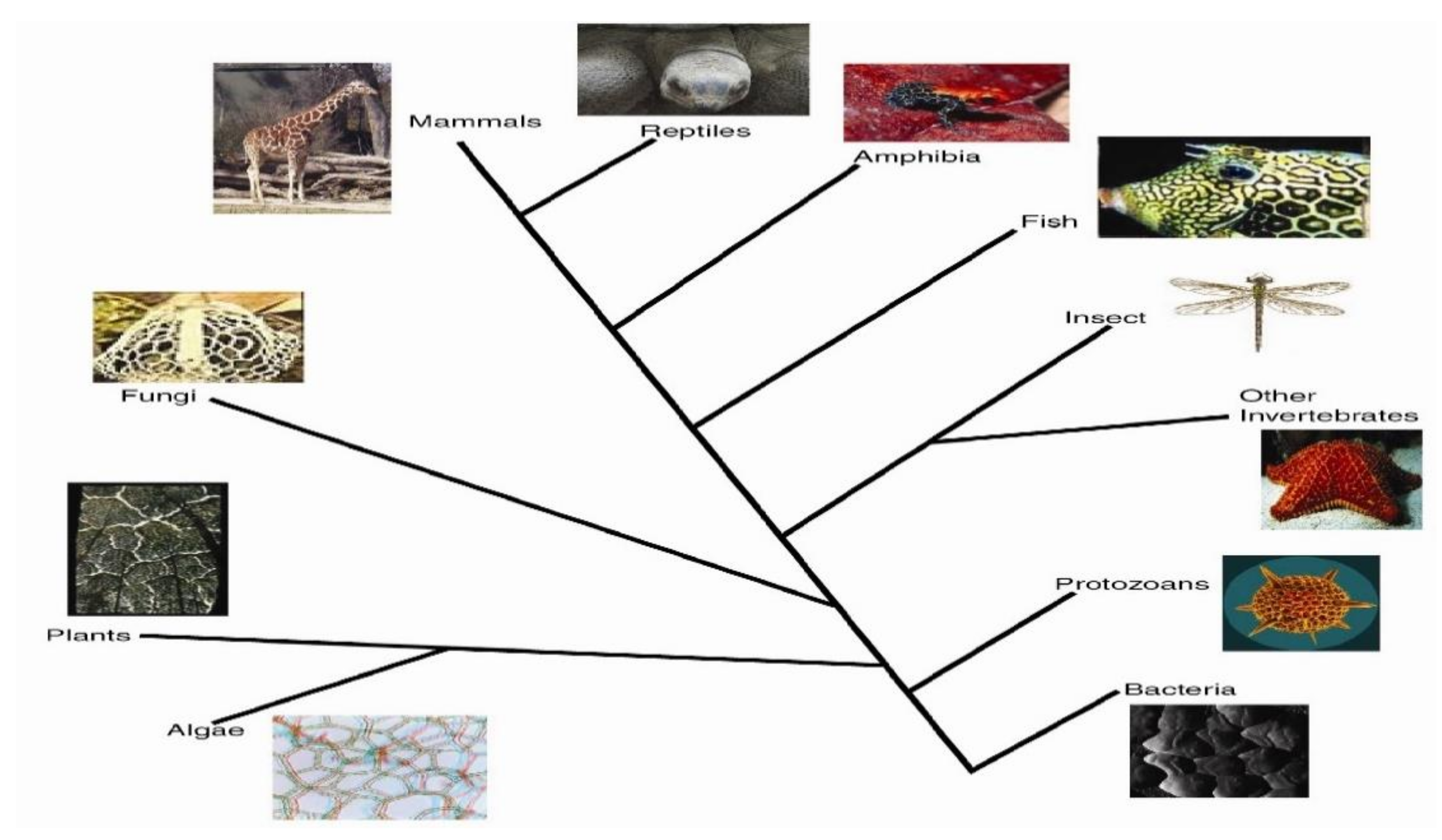
2.2. Phylogenetic Distributions

In addition to Voronoi tessellations observed at multiple scales as listed in Table 1, in Figure 6, the wide phylogenetic diversity of organisms with these patterns is shown.

2.3. Temporal Distributions

In addition to various sizes and a broad phylogenetic diversity, the biological patterns take vastly different times to form. For example, a mature tree canopy can take hundreds of years to reach maximal height and form the “canopy gaps” between adjacent large trees. On the other hand, a viral capsid can self-assemble in milliseconds. For a list of so such temporal variation, see

Table 2. Spatio-temporal variation in Voronoi tessellation patterns produced by different mechanisms in phylogenetically diverse contexts.

Biological Voronoi Pattern	Spatial Variation: Rough Potential Scale	Temporal Variation: Rough Estimate of Time of Formation
Rain forest canopy gaps	300 m to kilometers	Hundreds to thousands of years
Stony coral	About 1 m	Years
Talapia fish nesting territories	30 m	Days
Embryogenesis	5 mm to 10 m	Hours to 30 months gestation
Slime mold aggregation	5 cm	Hours
Quorum sensing biofilm	mm to cm	Minutes
Protein folding	Angstroms to nm	Nanoscends to milliseconds

. What almanacs, calendars, and clocks do you use that you think would be most helpful in measuring temporal patterns?

2.4. Space and Time Simultaneously

Not only do Voronoi patterns emerge over different scales, but they also persist for very different time periods. How are these correlated (see Table 2)? How should we think of biological patterns: as static or dynamic, persistent or evanescent, internal or external? In physics, much is made of the interaction of space and time. When we use a telescope, the light that impinges on our retina may have left a remote star millions of light years ago; thus, seeing far means that we are seeing into remote time; we are not seeing what is simultaneously occurring at that location. What about when we look in through a microscope? Frequently, we have to use a strobe light to pause the rapid motion of structures such as cilia or flagella. Similarly, if we make a movie at somewhat standard frames of reference such as 22 frames a second and if our shutter speed is a thousandth of a second, then we have missed 978/1000 (or roughly 98%) of what was going on. We psychophysically interpret our perception of the animation as continuous even when we rationally know that we have discretized time. Do we trust that our sampling is statistically reliable? There is a famous physics film developed by the former editor of Scientific American Phillip Morrison along with the famous husband-wife team of designers, Charles and Ray Eames, entitled Powers of Ten [17]. The movie starts with a couple having a picnic in Grant Park in Chicago near the shore of Lake Michigan. The camera zooms out in steps of ten until we can look back on our Milky Way galaxy as only one of many and inwardly until we reach the subatomic level. Correspondingly, we developed Figure 7 to illustrate that biologists have to deal with similar complexity in terms of orders of magnitude.

2.5. Topological Analyses

To analyze the topological question of “who is the closest neighbor to whom?” rather than the geometry addressed above, another Ukrainian mathematician Boris Nikolaevich Delaunay (later published under the transliteration Delone) published a triangulation in 1934 [18] that is the dual of the Voronoi tessellation. Again, many synonyms abound; Patel et al. [10] referred to Delaunay triangulations as the “underlying topology of cell-cell connections.” This qualitative question of “who is the closest neighbor to whom?” is useful for testing whether associations between neighbors are next to one another or not. In order to do so, let us examine two classic data sets used in spatial statistics: cancerous and noncancerous amacrine cells (see Figure 8) and hamster tumor cells (see Figure 9). The Delaunay triangulation is tricolored separately: for example, bivariate data such as on-off generates three kinds of edges: on-on, off-off, and on-off. If p = the frequency of on points and q = the frequency of off points, then the a priori expected distribution of the three edges will be the familiar binomial distribution: p ² + 2pq + q² =1 which can be tested via a Chi-squared goodness of fit test with 1 degree of freedom (loss of a second degree because of the additional constraint that p + q = 1).

In this case, we can test the distribution of the three kinds of edges with a Chi-squared test for bivariate data if we presume a binomial distribution. There were 294 observed amacrine cells, of these 152 were in the on state and 142 were in the off state. When we examine the Delaunay edges in Figure 5c we found a total of 840 edges,

Thus, the binomial distribution we would expect is:

Expected On-On edges = (152/294)² T = (0.267) 840 = 224.5 On-On edges

Expected On-Off edges = 2 (152/294) (142/294) T = (0.499) 840 = 419.5 On-Off edges

Expected Off-Off edges = (142/294)² T = (0.233) 840 = 196 Off-Off edges

Results:
Observed:		Expected:
On-On:	161	On-On:	224.5
On-Off:	527	On-Off:	419.5
Off-Off:	152	Off-Off:	196

The result of the Chi-Squared analysis {χ2 = Σ (observed – expected)²/expected} was 55.06, which using a standard statistical table with a one degree of freedom indicates that the probability is less than 0.001 that this deviation from randomness could occur by chance; therefore, we conclude that there is significant clustering in the data.

On the other hand, let us look at the nuclei of two types of cells, • are the Pyknotic nuceli, and * are the metaphase nuclei from hamster tumor cells (Figure 9).

Using the information of the colored Delaunay triangulation, we observed 485 metaphase-metaphase Delaunay edges, 333 metaphase-Pyknotic Delaunay edges, and 53 Pyknotic-Pyknotic Delaunay edges. This gives a total of 871 Delaunay edges, which is then used in finding the expected number of edges in each group. The equations below were then used to find the expected numbers.

Expected Pyknotic-Pyknotic edges = (77/313)² T = (0.061) 871 = 53 Pyknotic-Pyknotic edges

Expected metaphase-Pyknotic Delaunay edges = 2 (77/313) (236/313) T = 2 (0.246) (0.754) 871 = (0.371) 871 = 323 metaphase-Pyknotic edges

Expected metaphase-metaphase Delaunay edges = (236/313)² T = (0.569) 871 = 496 Metaphase-metaphase edges

Results:
Observed		Expected
Pyknotic-Pyknotic edges:	53	Pyknotic-Pyknotic edges:	53
Metaphase-Pyknotic edges:	333	Metaphase-Pyknotic edges:	323
Metaphase-Metaphase edges:	485	Metaphase-Metaphase edges:	496

Obviously, even without calculations, these expected values look close to observed. The result of the Chi-Squared analysis was 0.225, which using a standard statistical table with a one degree of freedom indicates that the probability falls between 0.9 and 0.8 that this deviation from randomness could occur by chance; therefore, we cannot reject the null hypothesis conclude that there is no evidence of clustering in the data.

Thus, Ka-me makes analyses of the spatial point distributions of both single kinds of generator points such as tests of a radiolarian as well as bivariate data (on-off, metaphase-pycnotic) easy and rapid for even quite large data sets. The implementation of multiple indices is helpful because there is a wide literature on how each behaves in a variety of circumstances.

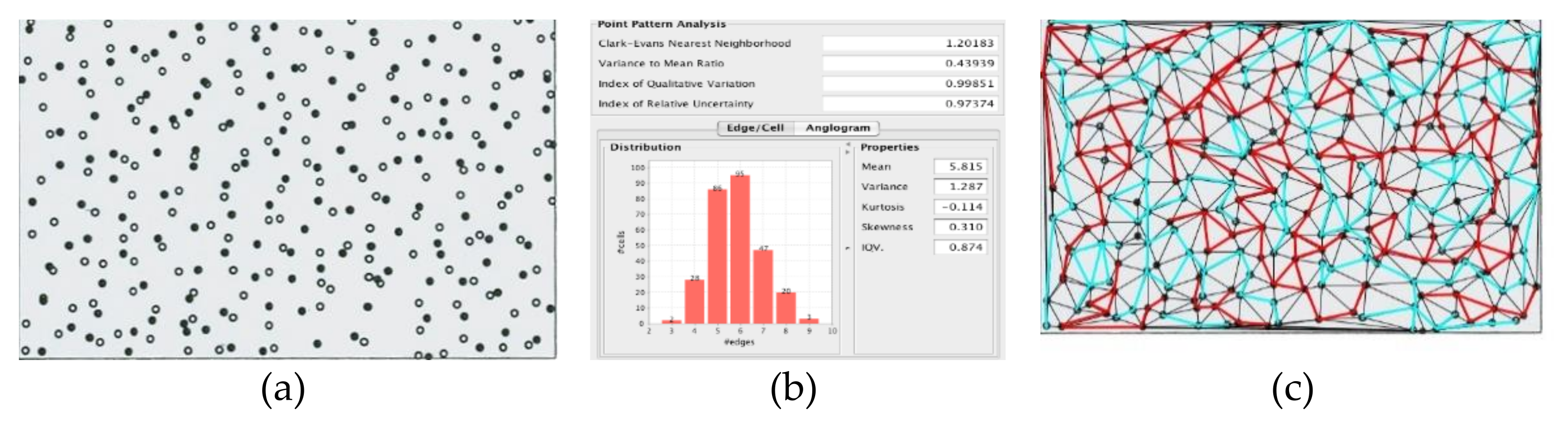
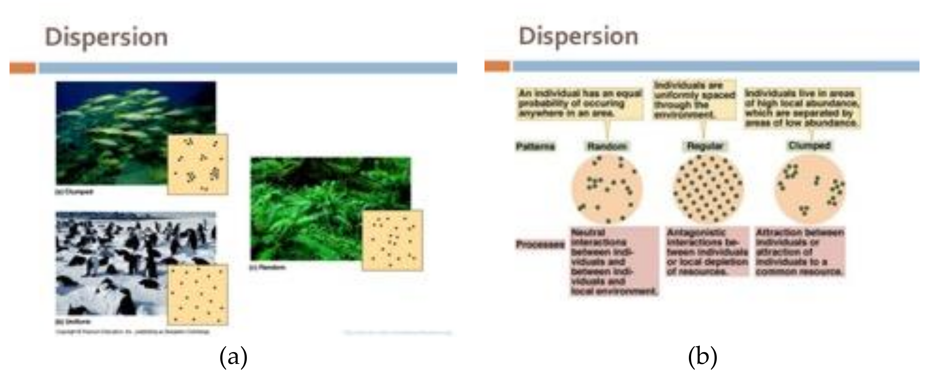
2.6. Spatial Statistics

How are the Voronoi generator points themselves distributed? Generally, we classify spatial point distributions into four categories:

(a)

Uniformly;

(b)

Randomly;

(c)

Clustered,

(d)

Disperse (see Figure 10);

Even though this is obviously a discretization and there must be continuous patterns in between these recognizable patterns.

In Ka-me, we distinguish these patterns by the use of two different spatial statistics: the Clark-Evans nearest neighborhood test and the variance to mean ratio test. We initially implemented two other four tools most commonly used by ecologists, the Index of Quantitative Variation and Index of Relative Uncertainty but did not find that they added anything new to the other two. The Clark-Evans nearest neighborhood (Figure 11a) behaves quite well in biological image analysis; however, since the variance to mean ratio test (Figure 11b) is not dimensionless, it is heavily dependent upon the pixel size of any particular analysis. We included the variance to mean ratio test in Ka-me only because it is the most widely used metric even though it is less informative in this implementation.

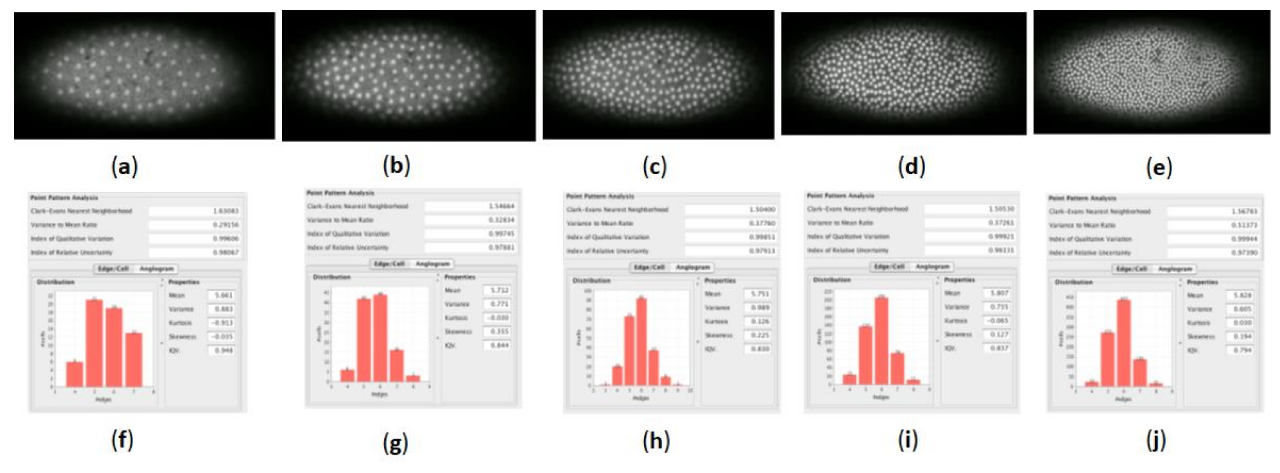
We have used Ka-me to analyze five generations in a dividing epithelium (a Drosophila embryo) from a beautiful film by Thomas Gregor [19] at Princeton produced with laser confocal microscopy (see Figure 12). Even though we know that incredible differentiation and distribution of morphogenetic signals are producing patterns that lead to fate maps to adult tissues of these cells, there is no apparent clustering of nuclei over the whole embryo during these divisions.

The Clark-Evans dispersion index uses the measurements from the Delaunay triangulation to calculate the dispersion index of the sample by comparing the expected mean summation of distances from each individual to its nearest neighbor by the observed mean distance (Clark and Evans [21]; Simberloff modification of the Clark-Evans measure: Cox [22]. The Clark-Evans index of dispersion ranges from 0, maximally clustered, to 1.0 indicating a randomly dispersed population, to 2.1491 indicating a uniform pattern. At 2.1491, all polygons are hexagonal, because perfectly regular spacing occurs when polygons are hexagonal in shape [21,22]. The general rule of thumb when using the Clark-Evans dispersion index is if the value of R is equal to 1, then we infer that the points are randomly dispersed. If R is significantly greater than 1, then the population is more uniformly dispersed. Finally, if R is significantly less than 1, then we infer that the points are clustered. In Figure 12, the Clark-Evans dispersion index values were very close to 1 (1.03 in one case); therefore, we have no evidence of clustering or repulsion of nuclei in these embryos.

Similarly, the variance to mean ratio test is interpreted in a very similar way: if the variance/mean ratio is equal to 1, the points are randomly distributed. If the variance/mean ratio is significantly greater than 1, the points are considered to be clustered. Finally, if the ratio is significantly less than 1, the points are more uniformly distributed. In general, values above 2 in either direction are often used as cut off points for rejecting random assumptions. The Ka-me value of the variance to mean ratio test did not exceed 1.44 for any of the images; therefore, again, we did not infer anything other than a random distribution of nuclei in these embryos.

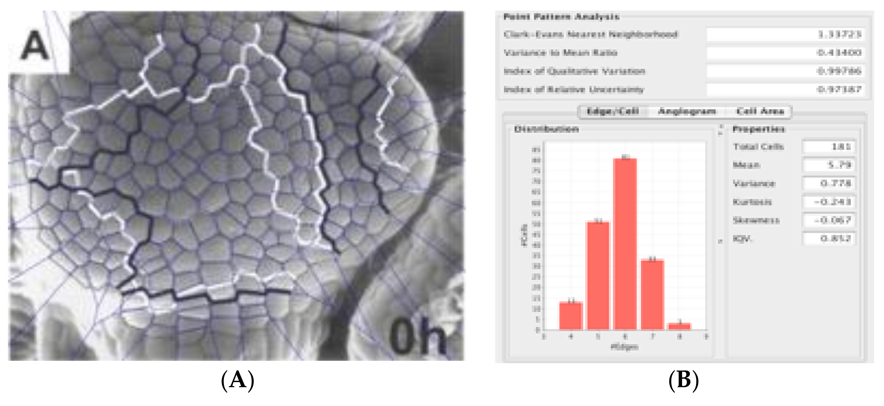
We were able to find a case where the Voronoi tessellation of a biological epithelium produced values of both measures that were not random (see Figure 13).

Recently, we saw a beautiful illustration of this spatial analysis in a medical examination of fast and slow twitch muscles (Figure 14).

2.7. Geometric Analyses: Area, Centroidality, Circularity, and Perimeter

Biologists have studied epithelial tissues from many species for hundreds of years. For the tessellations that they observed, they made inferences about empirical geometric measurements on their images (

Table 3. Eight analyses of the distribution of the sides per polygon of Voronoi tessellations that widely appear in the biological literature.

Eight Hypotheses/Rules/Properties That We Test:
	Name of Hypothesis/Rule/Property	Phenomena Observed/Tested
1	Euler’s Law	Vertices minus edges plus faces = 2
2	Distribution of Polygons	Are the number of sides of Voronoi polygons in the tessellation normally distributed?
3	Lewis’s Law	Are the areas of Voronoi polygons in the tessellation positively correlated with their number of edges?
4	Desch’s Law	Are the perimeters of Voronoi polygons in the tessellation positively correlated with their number of edges?
5	Aboav-Weaire Law	Is topological charge conserved?
6	Pitteway Violations	Do any edges of the Delaunay dual of the Voronoi tessellation cross more than one Voronoi edge?
7	Centroidality	Does a Voronoi polygon’s generator point fall on its gravitational center?
8	Errera’s Rule	Are the areas of the Voronoi polygons positively correlated with that of one of their immediate neighbors? (In successive generations of a tissue, did the average area of cells decrease by half in each subsequent generation?)

).

2.7.1. Errera’s Rule

In the 19th century, Errera [25] postulated that the area of daughter cells would be half that of the parent cell (the assumption of equal division of the cytoplasm of the parent cell to form the daughter cells). Six recent papers [26,27,28,29,30,31] have extended Errera’s rule to examine some other potential models (Sachs, Hofmesiter, Heinowicz, Besson and Dumais, Gibson, minimum degree, minimum random wall, shortest) of the cleavage plane of epithelial cells. Since on a static diagram, we do not know from one tissue with the cells going through simultaneous cell division to the next, which particular parent cells gave rise to particular daughter cells in the subsequent image, we test whether the mean areas of generations are halved in each subsequent division. We tested this on three different species: fruit flies (Drosophilia melanogaster) [data from [23]; Figure 15a] and flour beetles (Tribolium castenenum) [data from [32]; (Figure 15b)], and mustard plant (Arabipdopsis thaliana). In all three cases, the observed areas of sequent divisions were very close to the halves predicted by Errera [25].

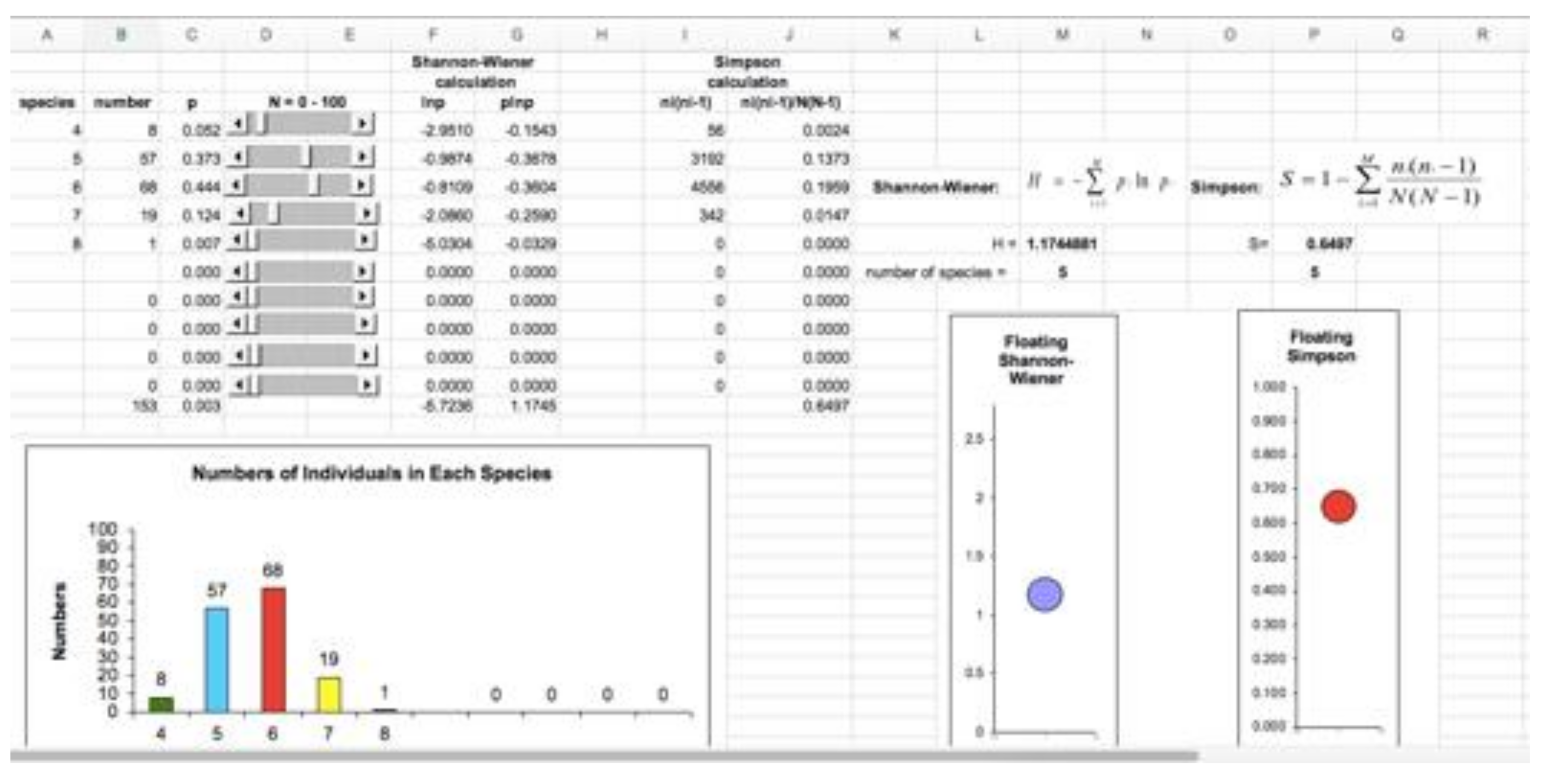
2.7.2. Voronoi Entropy

While most investigators of Voronoi entropy simply employ the Shannon formula for computation, our spreadsheet model [34] (Figure 16) calculates both the Shannon and Simpson diversity index. Bormashenko, Frenkel, and Legchenkova [35] state that the Voronoi Entropy “represents the averaged Shannon measure of ordering for 2D patterns.” It is an intensive rather than an extensive measure. For our three divisions of Triboleum casteneum the values of the Shannon measure of Voronoi Entropy were 1.23 for Division 10, 1.95 for Division 11, and 1.17 for Division 12. Therefore, we saw no monotonically increasing or decreasing trend. This is not surprising because, even though the number cells nearly doubles with each synchronic division (see Errera’s Rule [25]), as Bormashenko, Frenkel, and Legchenkova [35] furthermore point out “that the Voronoi entropy of the pattern characterized with the given and constant 2D order does not depend either on the area of the pattern nor on the number of seed points (of course, this is true, when the boundary effects are neglected). In contrast, the entropy is an extensive thermodynamic value, in other words it grows with an increase in the number of particles constituting the system.”

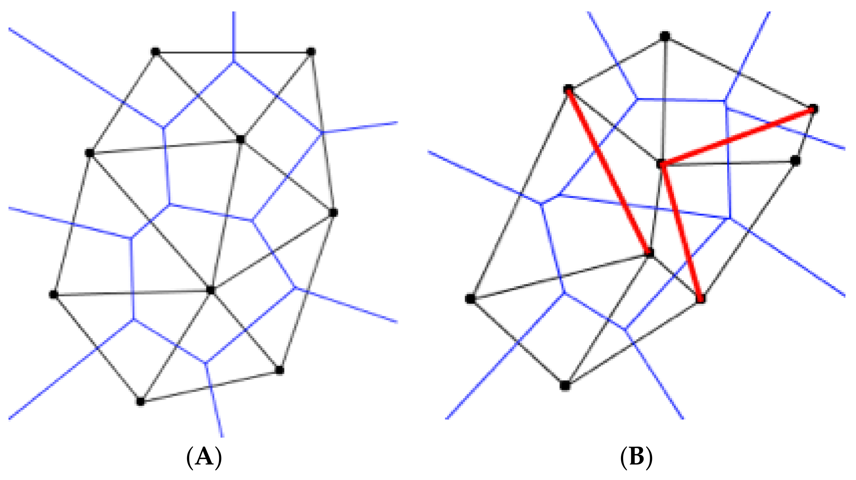
2.7.3. Pitteway Violations

When the Delaunay triangulation and Voronoi diagram are placed on top of one another, and the edges of the Delaunay triangulation and the Voronoi diagram of the same pair of points (“dual edges”) cross through each other forming the Pitteway triangulation [36,37,38,39]. A Pitteway violation occurs if the edges created by the Delaunay triangulation and Voronoi diagram from the same pair of points do not cross each other, this is usually observed by the Delaunay edge crossing over two Voronoi edges that are not generated from the respective points. Figure 17A shows a Voroni tessellation whose Delaunay dual has no Pitteway violations. Figure 17B shows the violations of the Pitteway triangulation, marked in red, from the overlay of the Delaunay triangulation onto the Voronoi diagram. The mean number of edges that a sample has is calculated by summing the number of edges per each point divided by the number of points in the sample (Cox 1996). The mean number of edges, proportion of hexagons, and the Clark-Evans dispersion index are all calculated using the number of edges that a point has. The proportion of Pitteway violations is a test of topological data, which in this case is the mathematical structures that are used for the relationships between objects, to determine the irregularities in the sample. These tests have close relation to each other, therefore, I hypothesized that the mean number of edges, proportion of hexagons, proportion of Pitteway violations, and the Clark-Evans dispersion index are highly correlated in biological samples.

Can we generalize this empirical relationship to have a more solid footing? Gold [40] had pointed out that “any triangulation of a regular pentagon includes a central isosceles triangle such that a point p near the midpoint of one of the triangle sides has its nearest neighbor outside the triangle” does not support a Pitteway triangulation. Herein we prove that if any Voronoi polygon has an interior angle less than 90 degrees, then a Pitteway violation will occur. In exercise 4.29 (page 110), in Satyan L. Devadoss and Joseph O’Rourke’s (2011) book: Discrete and Computational Geometry (Princeton University Press) [41], they challenge readers to show why not every Delaunay dual of a Voronoi tessellation satisfies the Pitteway condition, but they do not provide a general proof. Furthermore, we will assert that using the interior minimal angles of the convex polygons in a Voronoi tessellation can be used in a multivariate prediction of the topological properties (number of edges per polygon) from geometric properties (area, perimeter) than univariate rules described above (Lewis Law and Desch’s Law).

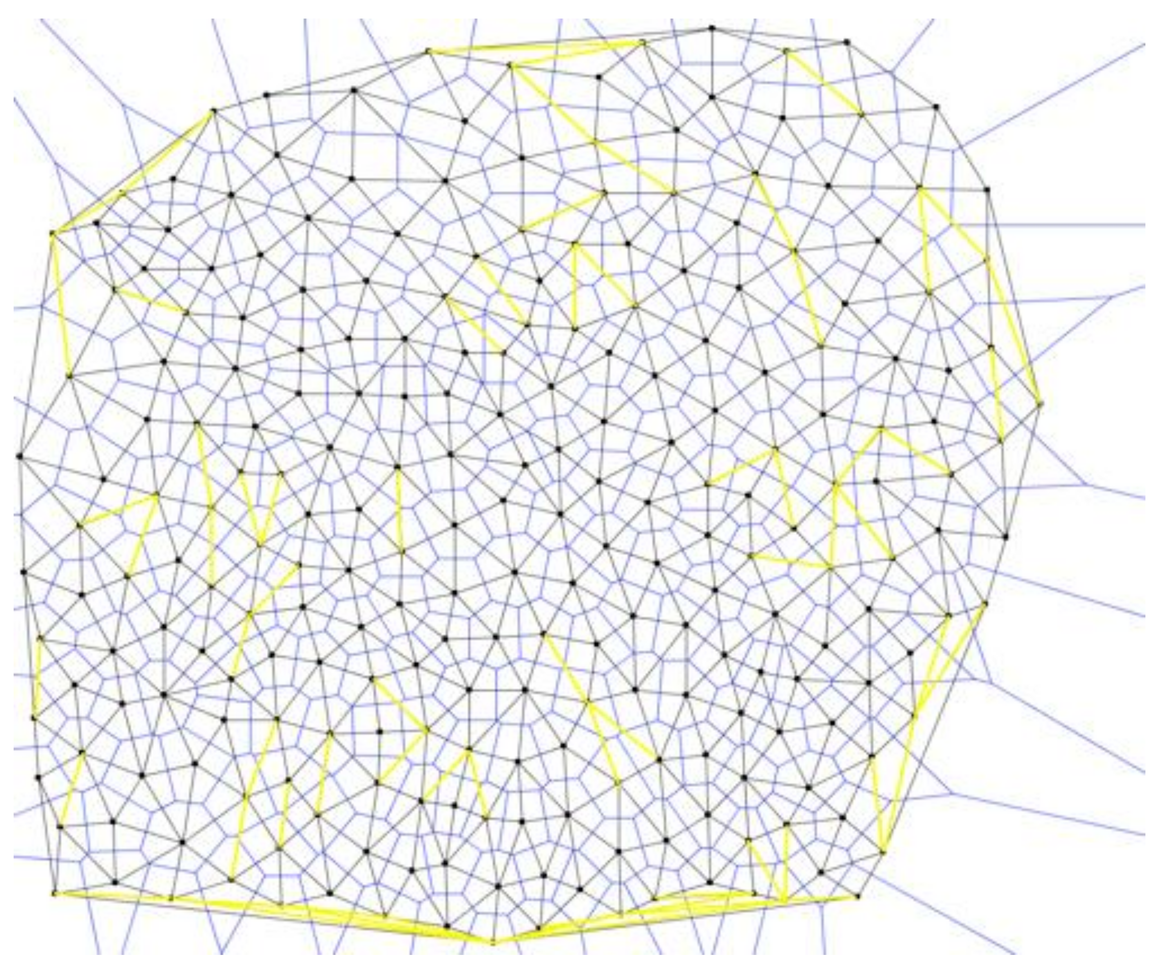
First, from a biological image analysis perspective let us examine actual biological images for Pitteway violations. In Figure 18, Patel et al. [18] reported on Voronoi tessellations that matched the configurations of convex cells in epithelia of Drosophila melanogaster embryonic epithelia. We analyzed it for the presence of Pitteway violations.

Note that 68 out of 707 edges violated the Pitteway condition; in other words, 9.62% of the Patel et al. [33] data had Pitteway violations. Please note that most violations occurred on the outer edges. We wondered whether this way due to photographic aberrations because the embryo is ovoid in structure and so the planar photograph is primarily distorted on the margins. This led us to our work on 3D nanotomography of radiolarian tests because we had a crystalline biological polyhedron with polygonal tessellations over its surface where we could avoid photographic aberrations [42,43].

Above in Figure 12a–e, we showed five generations of successive divisions of Drosophila embryogenesis from film by Thomas Gregor [14]: (a) 3 s (b) 8 s (c) 14 s (d) 34 s (e) 42 s; (f–j) along with the corresponding indices of dispersion and histographic frequencies of edges per polygon in the respective Voronoi tessellation for each of the five images using nuclei as Voronoi generator points in Ka-me. 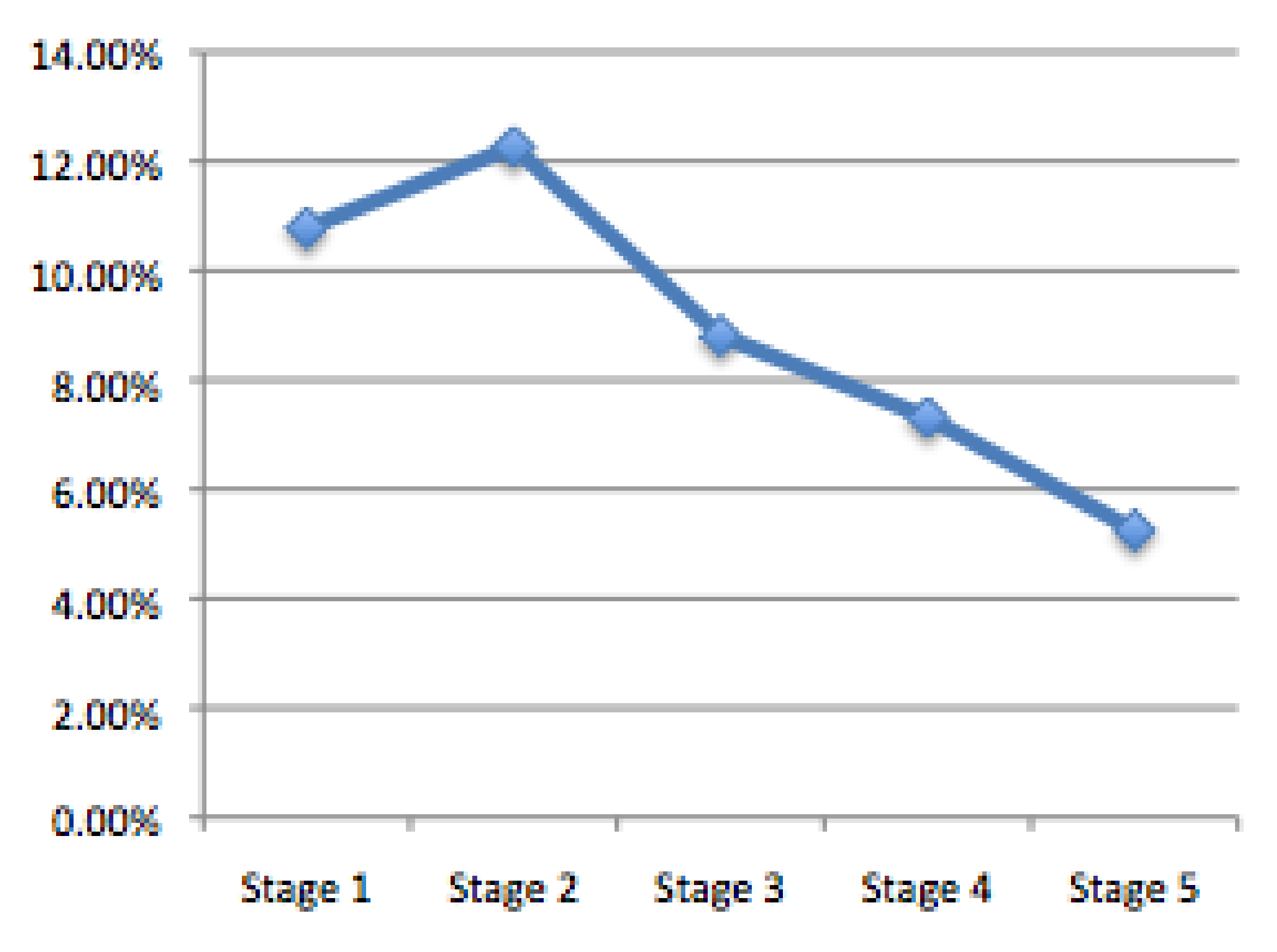(From [20]). We them analyzed each successive division for Pitteway violations (Figure 19):

After Stage 2, Pitteway Violations decrease with the increase in the number of cells in an area of the image. While more cells exist within in the same area, they are becoming more stable, and most cell-cell junctions determine which nuclear signals would affect neighboring cells. The result is statistically significant (Figure 20) as we noticed that in the polygonal distributions (Figure 12) that over successive generations that more hexagonal cells were prevalent in the Voronoi tessellations.

To better understand what was going on, we sought a general insight into which kinds of individual convex polygons in a Voronoi tessellation are correlated with Pitteway violations in the Delaunay dual. We found the following characterization.

Theorem 1.

For a finite set P of points in general position in the plane, Pitteway Violations occur precisely where there is an acute angle in the Voronoi Diagram.

“General position” means that the points avoid a few configurations that are inconvenient but also extremely unlikely (probability measure zero):

(i)

No three points of P are colinear;

(ii)

No circle contains more than three points of P, and;

(iii)

A circle with two points of P at antipodes contains no third point of P (Figure 21).

A finite set P of points in general position defines a unique Delaunay triangulation and dual Voronoi diagram.

Proof of Theorem 1.

Let C be a polygonal cell in the Voronoi diagram where the “seeds” are the finite set P and let P₀ ∈ P be the seed for C. Let v be a vertex on its boundary of C where two consecutive sides meet and let α and β be the angles that those sides make with the line segment vP₀. Each side of C is equidistant from P₀ and another seed vertex P_i, so if that side is extended to a line then it is perpendicular to and bisects the line segment P₀P_i. Figure 16 shows the seeds P₁, P₂ that are opposite to P₀ across the sides incident to v. By duality, P₀P₁ and P₀P₂ are edges in the Delaunay triangulation of P. P₀ and P₁ are the closest seeds to one side incident to v and P₀ and P₂ are the closest seeds to the other side incident to v, so v is equidistant from all three and no other seeds are closer to v. Since the seeds P are in general position, there is no fourth seed at that distance from v, and so it follows that v is incident to a total of three edges of the Voronoi diagram. Then, by duality, P₁P₂ is an edge of the Delaunay triangulation. There is a Pitteway violation here if and only if 2α + 2β < π. (Since the points P are in general position, the angle P₁vP₂ cannot equal π.) The internal angle of C at v is clearly α + β, so we have a Pitteway violation here if and only if that angle is less than π/2. □

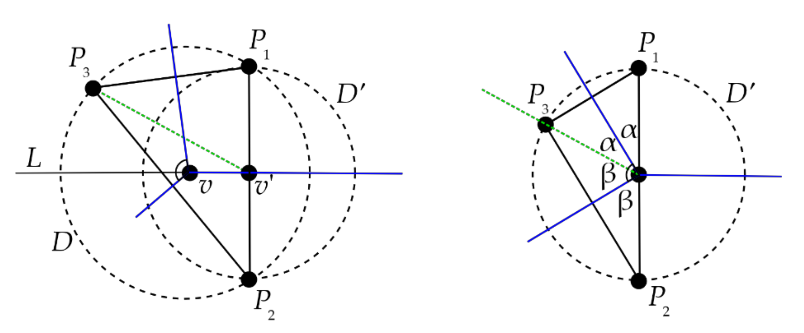
It is well-known that the Gabriel graph for a given set of points is a subgraph of its Delaunay triangulation, with the difference being precisely those edges which are Pitteway violations ([44]; also see Lemma 2 in [45]). Using this connection, we can give an alternative proof of the previous theorem (Figure 22).

Proof of Theorem 1 (sketch).

It is well-known that the Gabriel graph for a given set of points is a subgraph of its Delaunay. Let P₁, P₂ ∈ P such that P₁P₂ be an edge in the Delaunay triangulation. Then there is a disk D with P₁, P₂, and a third seed P₃ on its boundary. The center of D is a vertex v of the Voronoi diagram which is incident to three edges that lie between each pair of the seeds from P₁, P₂, P₃. Let D’ be the disk such that P₁P₂ is the diameter of D’ and let v’ be its center (the midpoint of P₁P₂). Then P₁P₂ is in the Gabriel graph of P if and only if D’ contains no seeds for P in its interior, and there is a Pitteway violation here otherwise. Let L be the line that bisects P₁P₂ and is perpendicular to it; then L contains v and v’.

Slide P₃ along the line through v’P₃ until it lies on the boundary of D’; this causes v to slide over to v’ and D to change until it equals D‘. Then two of the edges of the Voronoi diagram will meet at v at an angle α + β with 2α + 2β = π as shown in Figure 17, which is a right angle. Sliding P₃ back to its actual position will increase or decrease the angle that was α + β, depending on whether P₃ moves out or in to D’, causing the angle to be obtuse and P₁P₂ to be in the Gabriel graph, or making the angle acute and creating a Pitteway violation. □

After learning of the 90° requirement for Pitteway violations, we began to measure all of the interior angles of every convex polygon in Voronoi tessellations of epithelial cells of Drosophila melanogaster and Tribolium casteneum. Instead of assuming that the Pitteway violations were due to problems with the curvature of the embryo deforming cells on the perimeter of two-dimensional microphotographs, we found that Pitteway violations occurred even central to some images. In

Table 4. Regression analysis of flour beetle cell divisions: 10, 11, and 12.

R2 Values in Linear Regression Relationships.
	Division 10	Division 11	Division 12
Deasch’s Law (perimeter)	0.0015	0.0497	0.0840
Lewis’ Law (area)	0.0952	0.1530	0.1578
Circularity	0.4141	0.2217	0.1261
Smallest Angle	0.7549	0.6212	0.5118
Smallest Angle + Circularity	0.7583	0.6213	0.5120

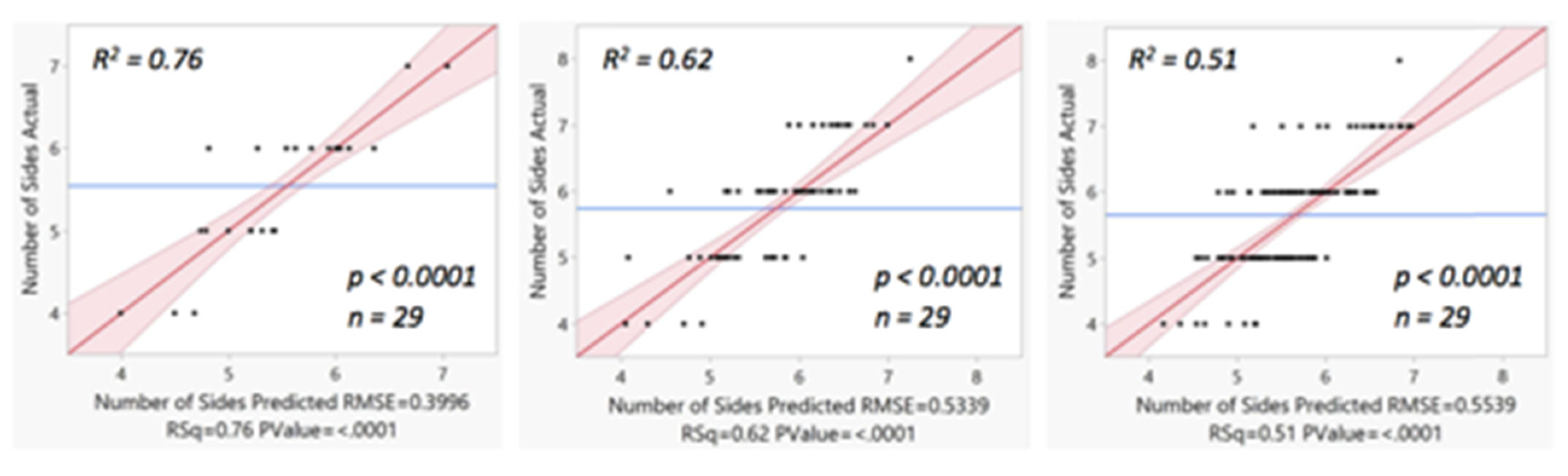
, we show that the smallest angle of the convex polygons in Voronoi tessellations of Tribolium casteneum is a much better predictor of the number of sides of the convex polygons in the Voronoi tessellation. In a multivariate regression, we could improve the R-square value of the regression slightly by employing circularity (recall that has information on areas and perimeters within its measurement) as well as the smallest angle information.

While the linear regressions for all five models were significantly significant, note that the smallest angle plus circularity produced a much better prediction of the number of sides of the convex polygons in these Voronoi tessellation than either Desch’s Law or Lewis’s Law which have been historically used throughout a wide swath of biological literature. Therefore, we suggest that the use of smallest angle alone or the smallest angle plus circularity relationship to the number of sides of the convex polygons in these Voronoi tessellation be called a “Pitteway Law” and urge colleagues to measure the interior angles of their convex polygons.

In Figure 23 we show that the three multiple linear regression graphs of expected versus predicted the number of sides of the convex polygons in these Voronoi tessellation based upon using both the smallest angle plus circularity variables.

3. Conclusions

Phenomenological models of biological patterns have provided a major path for biologists to see the impact of point-point nearest neighbor effects in using of Voronoi tessellations to analyze features of the distribution of convex polygons in such tessellations. Simply by observing tessellations that have convex polygons with degree = 3 vertices, it can be inferred that these patterns primarily arose by some causal force that was operating in a nearest-neighbor interaction. A powerful series of topological and geometric measurements can be deployed to determine significant relationships between topological properties such as vertices, edges, and faces on the one hand and geometric measurements such as angles, areas, and perimeters on the other hand. Graph theorists have developed a wide variety of tools that involve triangulations, cycles, paths, neighborhoods, spatial distributions, and topological charges that let us explore these complimentary relationships between topology and geometry of tessellations. Herein we have demonstrated this versatility by using examples of Voronoi tessellations to examine the distribution of successful and unsuccessful bird nests, species of trees in a diverse forest, different cells in the eye, fast and slow-twitch vertebrate muscle fibers, radiolarian tests, and extensively of embryos of fruit flies (Drosophila melanogaster), flour beetles (Triboleum casteneum), and plants (Anagallis arvensis, scarlet pimpernel). While Lewis’s Law relating the areas of convex polygons in a Voronoi tessellation and Desch’s Law relating the perimeters of convex polygons in a Voronoi tessellation have been the most widely used relationships in the biological literature, we have shown herein that “Pitteway’s Law” relating the smallest angles of convex polygons in a Voronoi tessellation possess a significantly better regression model than either of these two “laws.” The causal basis of these relationships is being examined and both mechanical (surface energy [46]) and topological (number of sides [47]) are reported to have major impact on the formation of epithelial Voronoi tessellations. The need for determining these relationships have potential medical importance in developing quantitative models for differentiating between normal, benign, and metastatic tissues in cellular pathology assessments for diagnosis, treatment, and prognosis.

References

1. Churkin, A.; Totzeck, F.; Zakh, R.; Parr, M.; Tuller, T.; Frishman, D.; Barash, D. A Mathematical Analysis of RNA Structural Motifs in Viruses. Mathematics 2021, 9, 585. [Google Scholar] [CrossRef]
2. Sen, A.; Aschheim, R.; Irwin, K. Emergence of an Aperiodic Dirichlet Space from the Tetrahedral Units of an Icosahedral Internal Space. Mathematics 2017, 5, 29. [Google Scholar] [CrossRef] [Green Version]
3. Falcón, R.M.; Falcón Óscar, J.; Núñez, J. An Application of Total-Colored Graphs to Describe Mutations in Non-Mendelian Genetics. Mathematics 2019, 7, 1068. [Google Scholar] [CrossRef] [Green Version]
4. McCormick, B.H.; DeFanti, T.A.; Brown, M.D. Visualization in Scientific Computing. Computer Graphics 1991, 21, 14. [Google Scholar] [CrossRef]
5. Gilbert, J.K. Visualization: A metacognitive skill in science and science education. In Visualization in Science Education; Springer: Dordrecht, The Netherlands, 2005; pp. 9–27. [Google Scholar]
6. Aurenhammer, F.; Klein, R.; Lee, D.-T. Voronoi Diagrams and Delaunay Triangulations; World Scientific Publishing Company: Singapore, 2013. [Google Scholar]
7. Khiripet, N.; Khantuwan, W.; Jungck, J.R. Ka-me: A Voronoi image analyzer. Bioinformatics 2012, 28, 1802–1804. [Google Scholar] [CrossRef] [Green Version]
8. Honda, H. Description of cellular patterns by Dirichlet domains: The two-dimensional case. J. Theor. Biol. 1978, 72, 523–543. [Google Scholar] [CrossRef]
9. BioQUEST Curriculum Consortium. Available online: http://bioquest.org (accessed on 25 October 2021).
10. Honda, H.; Tanemura, M.; Nagai, T. A three-dimensional vertex dynamics cell model of space-filling polyhedra simulating cell behavior in a cell aggregate. J. Theor. Biol. 2004, 226, 439–453. [Google Scholar] [CrossRef]
11. Voronoi, G. Nouvelles applications des paramètres continus à la théorie des formes quadratiques. Deuxième mémoire. Recherches sur les parallélloèdres primitifs. J. Für Die Reine Und Angew. Math. (Crelles J.) 1908, 134, 198–287. [Google Scholar] [CrossRef]
12. Gibson, M.; Patel, A.B.; Nagpal, R.; Perrimon, N. The emergence of geometric order in proliferating metazoan epithelia. Nat. Cell Biol. 2006, 442, 1038–1041. [Google Scholar] [CrossRef]
13. Stalling, D.; Westerhoff, M.; Hege, H.-C. Amira: A highly interactive system for visual data analysis. In The Visualization Handbook; Elsevier: Amsterdam, The Netherlands, 2005; Volume 38, pp. 749–767. [Google Scholar]
14. Jones, J.; Adamatzky, A. Slime Mould Inspired Generalised Voronoi Diagrams with Repulsive Fields. arXiv 2015, arXiv:1503.06973. [Google Scholar]
15. Shirakawa, T.; Adamatzky, A.; Gunji, Y.-P.; Miyake, Y. On simultaneous construction of Voronoi Diagram and delaunay triangulation by physarum polycephalum. Int. J. Bifurc. Chaos 2009, 19, 3109–3117. [Google Scholar] [CrossRef]
16. Adamatzky, A.; Rachel, A.; Jeff, J.; Yukio, G. On Creativity of Slime Mould. In Advances in Physarum Machines: Sensing and Computing with Slime Mould; Adamatzky, A., Ed.; Springer International Publishing: Basel, Switzerland, 2016; pp. 813–830. [Google Scholar]
17. Schrader, P. Poetry of Ideas: The Films of Charles Eames. Film. Q. 1970, 23, 2–19. [Google Scholar] [CrossRef]
18. Delaunay, B.; Sur, L.S.V. Izvestia Akademii Nauk SSSR. Otd. Mat. i Estestv. Nauk 1934, 7, 793–800. [Google Scholar]
19. Gregor, T. Lateral and Cross Section Nuclear Cycles of a Drosophila Embryo. YouTube Video. 2017. Available online: https://www.youtube.com/watch?v=sfhxZCsDHsU (accessed on 25 October 2021).
20. Reinfleisch, J.P.; Jungck, J.R. Spatial point analysis: Correlations between geometric and topological data from biological samples. Beloit. Biologist. 2010, 30, 1–75. [Google Scholar]
21. Clark, P.J.; Evans, F.C. Distance to Nearest Neighbor as a Measure of Spatial Relationships in Populations. Ecology 1954, 35, 445–453. [Google Scholar] [CrossRef]
22. Cox, G.W. Nearest-Neighbour Relationships of Overlapping Circles and the Dispersion Pattern of Desert Shrubs. J. Ecol. 1987, 75, 193. [Google Scholar] [CrossRef]
23. Kwiatkowska, D.; Routier-Kierzkowska, A.-L. Morphogenesis at the inflorescence shoot apex of Anagallis arvensis: Surface geometry and growth in comparison with the vegetative shoot. J. Exp. Bot. 2009, 60, 3407–3418. [Google Scholar] [CrossRef]
24. Bag, S.; Conjeti, S.; Das, R.; Pal, M.; Anura, A.; Paul, R.R.; Ray, A.K.; Sengupta, S.; Chatterjee, J. Computational analysis of p63+nuclei distribution pattern by graph theoretic approach in an oral pre-cancer (sub-mucous fibrosis). J. Pathol. Informatics 2013, 4, 35. [Google Scholar] [CrossRef]
25. Errera, L. Über zellformen und siefenblasen. Bot. Cent. 1888, 34, 395–399. [Google Scholar]
26. Rivier, N. Benoit Dubertret and Gudrun Schliecker. The stationary state of epithelial tissues. In Dynamics of Cell and Tissue Motion; Alt, W., Deutsch, A., Dunn, G., Eds.; Birkhauser: Boston, MA, USA, 1997. [Google Scholar]
27. Besson, S.; Dumais, J. Universal rule for the symmetric division of plant cells. Proc. Natl. Acad. Sci. USA 2011, 108, 6294–6299. [Google Scholar] [CrossRef] [Green Version]
28. Shapiro, B.E.; Jonsson, H.; Sahlin, P.; Heisler, M.; Roeder, A.; Burl, M.; Meyerowitz, E.M.; Mjolsness, E.D. Tessellations and pattern formation in plant growth and development. arXiv 2012, arXiv:1209.2937. [Google Scholar]
29. Lipowczan, M.; Piekarska-Stachowiak, A. Comparison of empirical rules describing cell plate formation in 2D computer simulations of apical meristem in plants. J. Biol. Syst. 2014, 22, 61–71. [Google Scholar] [CrossRef]
30. Louveaux, M.; Julien, J.-D.; Mirabet, V.; Boudaoud, A.; Hamant, O. Cell division plane orientation based on tensile stress in Arabidopsis thaliana. Proc. Natl. Acad. Sci. USA 2016, 113, E4294–E4303. [Google Scholar] [CrossRef] [Green Version]
31. Jackson, M.; Duran-Nebreda, S.; Kierzkowski, D.; Strauss, S.; Xu, H.; Landrein, B.; Hamant, O.; Smith, R.S.; Johnston, I.; Bassel, G.W. Global Topological Order Emerges through Local Mechanical Control of Cell Divisions in the Arabidopsis Shoot Apical Meristem. Cell Syst. 2019, 8, 53–65.e3. [Google Scholar] [CrossRef] [Green Version]
32. Patel, A.B.; Gibson, W.T.; Gibson, M.C.; Nagpal, R. Modeling and Inferring Cleavage Patterns in Proliferating Epithelia. PLoS Comput Biol. 2009, 5, e1000412. [Google Scholar] [CrossRef] [Green Version]
33. van Drongelen, R.; Vazquez-Faci, T.; Huijben, T.A.; van der Zee, M.; Idema, T. Mechanics of epithelial tissue formation. J. Theor. Biol. 2018, 454, 182–189. [Google Scholar] [CrossRef] [Green Version]
34. Kokou, A.; Sybille, C.; Francie, C.; Phil, R.; Paul, S. Biodiversity. A module of the Biological ESTEEM Collection, Published by the BioQUEST Curriculum Consortium. 2006. Available online: http://bioquest.org/esteem/esteem_details.php?product_id=2769 (accessed on 25 October 2021).
35. Bormashenko, E.; Frenkel, M.; Legchenkova, I. Is the Voronoi Entropy a True Entropy? Comments on Entropy, Shannon’s Measure of Information and Boltzmann’s H-Theorem, Entropy 2017, 19, 48. Entropy 2019, 21, 251. [Google Scholar] [CrossRef] [Green Version]
36. Pitteway, M.L.V. Computer graphics research in an academic environment. Datafair 1973, 73, 471–478. [Google Scholar]
37. McLain, D.H. Two dimensional interpolation from random data. Comput. J. 1976, 19, 178–181. [Google Scholar] [CrossRef] [Green Version]
38. Okabe, A.; Boots, B.; Sugihara, K.; Chiu, S.N. Spatial Tessellations: Concepts and Applications of Voronoi Diagrams; John Wiley & Sons: Hoboken, NJ, USA, 2009; Volume 501. [Google Scholar]
39. El Shazly, A.E. On the Spatial Conservation of Roundabout Cairo Using Pitteway Graph. In Conservation of Architectural Heritage. Advances in Science Technology & Innovation (IEREK Interdisciplinary Series for Sustainable Development); Hawkes, D., Bougdah, H., Rosso, F., Cavalagli, N., Ghoneem, M.Y.M., Alalouch, C., Mohareb, N., Eds.; Springer: Cham, Switzerland, 2019. [Google Scholar] [CrossRef]
40. Gold, C.M. The practical generation and use of geographic triangular element data structures. In Proceedings First International Advanced Study Symposium on Topological Data Structures for Geographic Information Systems. Harvard Papers on Geographic; Dutton, G., Ed.; Information Systems, Vol. 5—Data Structures: Surficial and Multi Dimensional; Laboratory for Computer Graphics and Spatial Analysis, Harvard University: Boston, MA, USA, 1978; Volume 5, pp. 1–18. [Google Scholar]
41. Devadoss, S.L.; Joseph, O’.R. Discrete and Computational Geometry; Princeton University Press: Princeton, NJ, USA, 2011. [Google Scholar]
42. Wagner, R.C.; Jungck, J.R.; Van Loo, D. Sub-micrometer X-ray tomography of radiolarians: Computer modeling and skeletonization. Microsc. Today 2015, 23, 18–23. [Google Scholar] [CrossRef]
43. Jungck, J.R.; Wagner, R.; Van Loo, D.; Grossman, B.; Khiripet, N.; Khiripet, J.; Khantuwan, W.; Hagan, M. Art Forms in Nature: Radiolaria from Haeckel and Blaschka to 3D nanotomography, quantitative image analysis, evolution, and contemporary art. Theory Biosci. 2019, 138, 159–187. [Google Scholar] [CrossRef] [PubMed]
44. Howe, S.E. Estimating Regions and Clustering Spatial Data: Analysis and Implementation of Methods Using the Voronoi Diagram. Ph.D. Thesis, Brown University, Providence, RI, USA, 1978. [Google Scholar]
45. Matula, D.W.; Sokal, R.R. Properties of Gabriel Graphs relevant to geographic variation research and the clustering of points in the plane. Geogr. Anal. 1980, 12, 205–222. [Google Scholar] [CrossRef]
46. Kokic, M.; Iannini, A.; Villa-Fombuena, G.; Casares, F.; Iber, D. Minimisation of surface energy drives apical epithelial organisation and gives rise to Lewis’ law. bioRxiv 2019, 590729. [Google Scholar]
47. Odde, D. Getting Cells and Tissues into Shape. Cell 2011, 144, 325–326. [Google Scholar] [CrossRef] [Green Version]
Figure 1. Consider the nine images above: (a) tropical rain forest canopy; (b) reticulated giraffe; (c) Tilapia fish territories; (d) Chameleon head; (e) Galapagos tortoise forefoot; (f) Petoskey stone (a) fossilized stony coral); (g) pollen grain; (h) Thai breadfruit (Artocarpus altili)); and, (i) radiolarian. (Figure 1a,b,d,e,g from https://commons.wikimedia.org/ accessed on 25 October 2021). Figure 1c from (http://www.finterest.com.au/ accessed on 25 October 2021); Figure 1f–h by author. Figure 1i is from Haeckel’s Art Forms in Nature (http://www.rarebooksberlin.de/fileadmin/haeckel_artforms.pdf (accessed on 25 October 2021) and see also Wagner and Jungck-Microscopy of Radiolarians and Foraminiferans https://spark.adobe.com/page/lm464/ (accessed on 25 October 2021).
Mathematics 09 02726 g001
Figure 2. A screenshot of a Voronoi diagram tessellation generated by the software Ka-me which is superimposed on a medial axial transformation of the 3D nanotomography image of a test of a radiolarian generated with the software Amira. The blue lines are the edges of the Voronoi cells, and the light-yellow lines are the edges of Radiolarian test. The forty Voronoi cells lie within the convex hull as the edges of the polygons external to the convex hull extend beyond the rectangle containing the image. Only 5-, 6-, and 7-sided convex polygons are observed and notice that all junctions are Y-shaped (i.e., trigonal, vertices with degree = 3) which is illustrative of patterns generated by local, nearest neighbor interactions versus X-junctions produced by global intersecting lines (Figure 3).
Mathematics 09 02726 g002
Figure 3. Intersecting lines generate X-junctions (i.e., all vertices have degree = 4). The convex polygons generated are primarily three- and four-sided, although much less frequently five-sided (here a polygon with vertices ABCDE exists with five edges). Note that no six-sided convex polygons are generated.
Mathematics 09 02726 g003
Figure 4. A Voronoi tessellation was generated in Ka-me with random points and the circumcircles are overlaid. Note that each circumcircle has three adjacent Voronoi polygons’ generator points and the center of each circumcircle is the vertex shared by all three adjacent Voronoi polygons.
Mathematics 09 02726 g004
Figure 5. Voronoi diagram and Delaunay triangulation developed during slime mould growth. An approximation of a Voronoi diagram by slime mould on nutrient agar gel. (a) Sites of plasmodium inoculation represent planar data points to be sub-divided by edges of Voronoi diagram. (b), (c) Experimental snapshots of growing plasmodia. (d) Bisectors of Voronoi diagram are represented by loci of substrate not occupied by plasmodium, bisectors computed by classical technique are shown by straight lines. (d) Delaunay triangulation approximated by slime mould growing on non-nutrient substrate. Edges of Physarum—computed triangulation are represented by protoplasmic tubes; edges computed by classical algorithm are solid lines. [16].
Mathematics 09 02726 g005
Figure 6. A phylogenetic sampling of species that display Voronoi tessellation patterns on their exterior or in their colonial aggregate. Clockwise from lower left: the colonial algae Hydrodictyon, a canopy of teak trees from Thailand, a lacey stinkhorn fungus, a reticulated giraffe, a Galapagos tortoise, a reticulated frog, a trunkfish, a dragonfly (the wing pattern), a starfish, a radiolarian, and a bacterial biofilm.
Mathematics 09 02726 g006
Figure 7. Voronoi-like biological patterns exist across twenty-four orders of space and time.
Mathematics 09 02726 g007
Figure 8. (a) Observed distribution of amacrine cells. (b) Ka-me screenshot of the distribution of Voronoi polygons generated by using each amacrine cell as a generator point. (c) A colored Delaunay triangulation of neighboring amacrine cells. There are three kinds of edges depending upon the corresponding states of neighboring amacrine cells: on-on, off-off, and on-off.
Mathematics 09 02726 g008
Figure 9. (a) Hamster tumor cells data provided by Dr. W. A. Aherne (Department of Pathology, University of Newcastle upon Tyne). The 313 nuclei of two types of cells, • are the 77 Pyknotic nuceli, and * are the 236 metaphase nuclei. (b) Using the Ka-me_0_84 program, the points to create both a Voronoi diagram and Delaunay triangulation. (c) Edges shared by metaphase-Pyknotic, and dotted lines show the edges Pyknotic-Pyknotic cells share.
Mathematics 09 02726 g009
Figure 10. Patterns of point distributions in space: (a) three biological communities: fish swarm, penguins on ice, and corals. (b) Biological assumptions about each of these three patterns: random patterns are presumed to be the result of “neutral interactions between individuals and the local environment;” regular [uniform] patterns are presumed to be the result of antagonistic interactions between individuals or local depletion of resource; clumped patterns are presumed to be the result of attraction between individuals or attraction of individuals to a common resource. Source: https://www.slideshare.net/thelawofscience/population-growth-22514883 (accessed on 25 October 2021).
Mathematics 09 02726 g010
Figure 11. (a) Range of the Clark-Evans nearest neighborhood; (b) range of the variance to mean ratio test.
Mathematics 09 02726 g011
Figure 12. Five generations of successive divisions of Drosophila embryogenesis from film by Thomas Gregor [15]: (a) 3 s (b) 8 s (c) 14 s (d) 34 s (e) 42 s; (fj) corresponding indices of dispersion and histographic frequencies of edges per polygon in the respective Voronoi tessellation for each of the five images using nuclei as Voronoi generator points in Ka-me (from Reinfleisch and Jungck [20]).
Mathematics 09 02726 g012
Figure 13. (A) We superimposed a Voronoi tessellation onto an image of “the inflorescence shoot apex of Anagallis arvensis” (Kwiatkowska and Routier-Kierzkowska [23]). (B) Ka-me analysis of the Clark-Evans nearest neighborhood and variance to mean ratio for the Voronoi tessellation. Both of these measures fall outside the usual random range.
Mathematics 09 02726 g013
Figure 14. “Slow fibres are labelled in red and fast fibres in black. (A) In the BA a high tendency for slow cells to be isolated govern the organization of the tissue. This induces a homogenous distribution of both types of fibres. (B) In QA, there is no clear tendency in the organization. Slow fibres can appear isolated or grouped. The distribution is random,” Bag et al. [24].
Mathematics 09 02726 g014
Figure 15. Tests of Errera’s rule that successive cell divisions have one-half the mean areas of the previous generation for tissues with simultaneous divisions of all cells. The linear regression of the ln(A) is plotted for five successive divisions. (a) Fruit flies (Drosophilia melanogaster) (data from [33]); test of Errera’s ½ rule: R-squared = 0.87, p < 0.0001. (b) Flour beetles (Tribolium castenenum) (data from [31]]; violin plots of the areas of Voronoi cells in each of three successive divisions; the blue line connects the mean areas of each of the three generations; the red line is what would be expected if Errera’s rule was used to predict the means of successive generations.
Mathematics 09 02726 g015
Figure 16. The distribution of sides per convex polygon type have used to calculate both Shannon and Simpson equations for diversity (Voronoi entropy in this case). The results are illustrated above from using our spreadsheet in the BioQUEST ESTEEM Collection [36].
Mathematics 09 02726 g016
Figure 17. (A) A Delaunay dual superimposed upon a Voronoi tessellation where the Pitteway triangulation condition is satisfied, i.e., each edge of the Delaunay dual crosses one and only one edge of the Voronoi tessellation. In this picture, the polygonal cells have a more general shape in that most of the interior angles are not too different from a mean of the interior angles. In such cases, biological investigators infer stability of the epithelia. (B) Pitteway violations are shown in red on this Delaunay dual superimposed upon a Voronoi tessellation, i.e., each of the red edges of the Delaunay dual crosses more than one edge of the Voronoi tessellation. In this picture the polygonal cells have a less general shape in that several of the interior angles are very different from a mean of the interior angles. In such cases, investigators infer that the irregularity of the above cells in the epithelia cause the Pitteway violation in which cases biological and geographic investigators [40] have used the presence of such violations to infer that such cell packings are less stable.
Mathematics 09 02726 g017
Figure 18. We illustrate the distribution of Pitteway violations (yellow edges) in a Voronoi tessellation of the epithelium of embryonic cells of Drosophila melanogaster. Data provided by [33]. The image was entered in Ka-me to illustrate the edges of the Delaunay triangulation of the Voronoi tessellation that cross more than one Voronoi edge (i.e., Pitteway violations).
Mathematics 09 02726 g018
Figure 19. Plot of the per cent of Pitteway violations on the Delaunay dual of the Voronoi tessellations of successive divisions of an embryo of Drosophila melanogaster. Stage 1: 10.78%; Stage 2: 12.265%; Stage 3: 8.807%; Stage 4: 7.31%; and Stage 5: 5.25% [20]. Raw images were stills extracted from Thomas Gregor’s, Princeton University, YouTube video: early mitotic divisions in a Drosophila embryo URL: http://www.youtube.com/watch?v=XSKh-GLQn4E (accessed on 25 October 2021).
Mathematics 09 02726 g019
Figure 20. Parametric linear regression of the proportion of Pitteway violations with successive divisions of cells in the embryo of Drosophila melanogaster [20].
Mathematics 09 02726 g020
Figure 21. In the proof below, C is a Voronoi cell, v is one of its vertices, and P0, P1, and P2 are “seeds” of the Voronoi diagram. P0P1, P0P2, and P1P2 are edges in the Delaunay triangulation, although for clarity P1P2 has been omitted from the figure.
Mathematics 09 02726 g021
Figure 22. On the left, three blue edges from the Voronoi diagram meet at vertex v, with “seeds” P1, P2, and P3, such that P1P2, P1P3, and P2P3 are edges in the Delaunay triangulation. In the proof below, P3 slides along the green line until it reaches the boundary of the disk D’, which also moves v to v’ and moves D to D’; the result is pictured on the right.
Mathematics 09 02726 g022
Figure 23. Plots of observed versus expected number of sides of the convex polygons in these Voronoi tessellations of Troboleum casteneum embryos described above. The three multiple linear regression graphs of expected versus predicted are all significant and as shown in Table 4 are much better than angle of the other four models that were tested.
Mathematics 09 02726 g023