Article

Dynamics of Tumor-Immune System with Random Noise

by
Fathalla A. Rihan
1,* and
Chinnathambi Rajivganthi
2
1
Department of Mathematical Sciences, College of Science, United Arab Emirates University, Al-Ain 15551, United Arab Emirates
2
School of Applied Mathematics, Getulio Vargas Foundation, Rio de Janeiro 22250-900, Brazil
*
Author to whom correspondence should be addressed.
Mathematics 2021, 9(21), 2707; https://doi.org/10.3390/math9212707
Submission received: 9 October 2021 / Revised: 21 October 2021 / Accepted: 23 October 2021 / Published: 25 October 2021
(This article belongs to the Section Mathematical Biology)

Abstract

:
With deterministic differential equations, we can understand the dynamics of tumor-immune interactions. Cancer-immune interactions can, however, be greatly disrupted by random factors, such as physiological rhythms, environmental factors, and cell-to-cell communication. The present study introduces a stochastic differential model in infectious diseases and immunology of the dynamics of a tumor-immune system with random noise. Stationary ergodic distribution of positive solutions to the system is investigated in which the solution fluctuates around the equilibrium of the deterministic case and causes the disease to persist stochastically. In some conditions, it may be possible to attain infection-free status, where diseases die out exponentially with a probability of one. Some numerical simulations are conducted with the Euler–Maruyama scheme in order to verify the results. White noise intensity is a key factor in treating infectious diseases.

1. Introduction

A cancerous tumor grows with abnormal hormones, causing it to spread throughout the body and potentially spread to other organs or parts of the body. An initial stage is called a tumor, which does not spread. The highest death rate among all diseases worldwide is cancer because of such risk factors as drinking alcohol, smoking, being overweight, physical inactivity, irregular reproductive patterns, an unhealthy lifestyle, monetary development and urbanization. Tumor cells develop and grow in three stages: first, they escape the immune system; then, they reduce the extracellular matrix; and finally, they help blood vessels survive in their tissue by suppressing the extracellular matrix [1]. Cancer can be treated with a variety of methods, such as chemotherapy [2], radiotherapy [3], surgery or hormone therapy [4] to inhibit and eradicate tumor cell growth. Rihan et al. [5,6] explained the stability, optimal control and bifurcation results of the tumor-immune system with the interaction between tumor cells, natural killer cells and cytotoxic T cells, with time delays and the Michaelis–Menten functional response. The author in [7] discusses multiple delays effect on the interaction between brain tumors and immune components in conjunction with T11 (CD2) target administration as well as the conditions for the local stability of steady states, bifurcation results, and the maximum delay to keep limit cycles stable. Many other researchers have investigated tumor-immune models to understand how the immune system works and examine how immune cells eliminate tumors in different ways [8,9].
Recent studies incorporated different random noises into deterministic tumor-immune models in order to discuss the dynamical behaviors of the corresponding stochastic models (see [10,11]). Basically, the environmental fluctuations stimulate mainly the intrinsic growth rate of host, tumor cells and death rate of effector cells. Moreover, the modeling of such phenomena, stochastic differential equations (SDEs), are more suitable than deterministic models, which offer a more reasonable representation for discussing the long-term kinetics of cell population. Liu et al. [12] studied the dynamical behaviors of tumor-immune responses under chemotherapy treatment; deterministic and stochastic differential equation models were constructed to characterize the dynamical changes in tumor and immune cells. The deterministic model was extended to the stochastic differential equations (SDEs) model and the continuous-time Markov chain (CTMC) model, which accounts for the variability in cellular reproduction, interspecific competition, growth, death, immune response, and chemotherapy. Yang et al. [13] derived the global positive solution and qualitative behaviors of the tumor-immune model with the combination of pulsed immunotherapy, pulsed chemotherapy and white noise effect. Das et al. [14] investigated the deterministic and stochastic modeling of the tumor-immune system under Michaelis–Menten kinetics and also studied the stochastic permanence, global attractivity and weak persistence in mean. The authors in [15] discussed the threshold condition about immune strength for survival, extinction and weak persistence results of a stochastic tumor-immune system.
In this paper, white noise is incorporated into an existing deterministic tumor-immune model to analyze the dynamics of the system. The presence and uniqueness of the global non-negative solution of the stochastic tumor-immune model with a Holling type III functional response is investigated. Using a stochastic Lyapunov function combined with Ito’s formula, we provide a sufficient condition for determining the existing results of stationary distribution, weak persistence, and extinction of tumor cells. The rest of this paper is organized as follows: In Section 2, we formulate the tumor-immune model and study the existence of global positive solution. The stationary distribution and extinction results of this model are derived in Section 3 and Section 4. Some numerical simulations are given in Section 5 to verify the obtained theoretical results. Section 6 contains the conclusion.

2. Stochastic Model for Tumor-Immune Interaction

It worth mentioning here that deterministic models are assumed for tumor-immune interactions; however, there is increasing evidence that better consistency with some phenomena can be provided if the effects of random processes in the system are taken into account. One of the important facts about the impact of the environmental noise is that it can suppress a potential population explosion [16,17,18].
The interaction between cancer and the immune system (IS) has been investigated by many authors using deterministic mathematical models (see [19,20,21,22,23,24,25]). The challenge is to obtain the known biological features without making the mathematics too complex. We include here the following features: The immune system is a multifunctional multipathway. We, therefore, use two immune effectors. The cross-reactivity of the immune system is also taken into account. The model is given by the following:
T ˙ ( t ) = a T r 1 T E 1 r 2 T E 2 , E ˙ 1 ( t ) = d 1 E 1 + T 2 E 1 T 2 + k 1 , E ˙ 2 ( t ) = d 2 E 2 + T 2 E 2 T 2 + k 2 ,
where T T ( t ) is the tumor cells; E 1 E 1 ( t ) , E 2 E 2 ( t ) are immune effectors with initial values of T ( 0 ) > 0 , E 1 ( 0 ) > 0 , E 2 ( 0 ) > 0 ; a is the growth rate of T ( t ) ; d 1 and d 2 are the decay rate of E 1 ( t ) and E 2 ( t ) , respectively; k 1 , k 2 represent the half saturation parameters; and r 1 and r 2 are the suppress rate of T ( t ) due to presence of E 1 ( t ) and E 2 ( t ) , respectively. All the above parameters are positive constants. The interaction terms in the second and third equations of system (1) satisfy the cross reactivity property of the immune system.
Lemma 1.
The solution of model (1) with non-negative initial values is non-negative.
Proof. 
The right hand sides of model (1) are continuous functions of dependent variables, and we can easily obtain the following:
T ( t ) = T ( 0 ) e x p 0 t a r 1 E 1 ( s ) r 2 E 2 ( s ) d s , E 1 ( t ) = E 1 ( 0 ) e x p 0 t d 1 + T 2 ( s ) T 2 ( s ) + k 1 d s , E 2 ( t ) = E 2 ( 0 ) e x p 0 t d 2 + T 2 ( s ) T 2 ( s ) + k 2 d s .
Therefore, it is clear from the above expressions that T ( t ) , E 1 ( t ) and E 2 ( t ) remain positive for all t > 0 if they initiate from an interior point of the following:
R + 3 = { T ( t ) , E 1 ( t ) , E 2 ( t ) : T ( t ) > 0 , E 1 ( t ) > 0 , E 2 ( t ) > 0 } .
Thus, R + 3 is positively invariant for (1). □
The steady states of the system (1) are the following:
( 0 , 0 , 0 ) ; ( d 1 k 1 / ( 1 d 1 ) , a / r 1 , 0 ) ; ( d 2 k 2 / ( 1 d 2 ) , 0 , a / r 2 ) .
We assume that in order to avoid the non-biological interior solution in which both immune effectors coexist, we have the following:
( d 1 k 1 / ( 1 d 1 ) ) < < ( d 2 k 2 / ( 1 d 2 ) ) .
According to the size of the tumor, the first steady state is naive, the second is memory, and the third is endemic. Analyzing the stability of naive state shows that they are unstable. Locally, the memory state is asymptotically stable if the following holds:
d 1 < 1 ,   and   d 1 < d 2 .
As long as the endemic state remains locally stable, the following holds:
d 2 < 1 ,   and   d 2 < d 1 .
Hence, we arrive at the following propositions:
Proposition 1.
When (4) is satisfied, then the memory state is asymptotically stable on the local level. Therefore, there is a bifurcation when d 1 = 1 .
Growing and interacting cancer cells differ depending on the cell properties, the immune system’s functioning, and the environment where the interaction occurs [26]. An individual’s overall health determines the environment in which the body operates. In order to discuss the impact of body environmental factors on the dynamics of cancer infection, we could extend the deterministic description of the tumor-immune interaction to include stochastic forcing, either additively or multiplicatively. Several researchers have studied mathematical models for studying epidemics in environmental noise, such as [27].
Some authors have introduced randomness into deterministic models to demonstrate the influence of environmental variation on biological systems by taking this into consideration; see [28,29]. For more realistic situation of the development process of the disease, we incorporate the effect of randomization within host by introducing nonlinear perturbation on the natural death rate with white noise into each equation of model (1). The parameters associated with the tumor-immune system are not certain, but the interval to which it belongs can easily be determined. We therefore suggest the following stochastic model:
d T ( t ) = ( a T r 1 T E 1 r 2 T E 2 ) d t + σ 1 T ( t ) d W 1 ( t ) , d E 1 ( t ) = ( d 1 E 1 + T 2 E 1 T 2 + k 1 ) d t + σ 2 E 1 ( t ) d W 2 ( t ) , d E 2 ( t ) = ( d 2 E 2 + T 2 E 2 T 2 + k 2 ) d t + σ 3 E 2 ( t ) d W 3 ( t ) ,
where σ 1 2 , σ 2 2 , σ 3 2 are intensities of the environmental white noises. W 1 ( t ) , W 2 ( t ) , W 3 ( t ) are mutually independent standard Brownian motions with W i ( 0 ) = 0 ( i = 1 , 2 , 3 ). We define the basic concepts of probability theory and SDEs. Let ( Ω , F , { F t } t 0 , P ) be complete probability space with filtration { F t } t 0 satisfying the usual conditions. See more details about Ito’s formula (see [16,30,31]).
Let y ( t ) be a regular time-homogeneous Markov process in R n defined by SDE:
d y ( t ) = f ( y ( t ) ) d t + g ( y ( t ) ) d W ( t ) .
The diffusion matrix of the process y ( t ) is described as A ( y ) = ( b i j ( y ) ) , b i j ( y ) = g i ( y ) g j ( y ) .
Lemma 2
(Ref. [32]). The Markov process y ( t ) has a unique ergodic stationary distribution π ( · ) if there exists a bounded open domain D R n with regular boundary Γ , having the following properties:
i.
The diffusion matrix A ( y ) is strictly positive definite for all y D .
ii.
There exists a non-negative C 2 function V such that L V is negative for any R n D .
Theorem 1.
Model (6) has a unique positive solution ( T ( t ) , E 1 ( t ) , E 2 ( t ) ) on t 0 with ( T ( 0 ) , E 1 ( 0 ) , E 2 ( 0 ) ) R + 3 , and the solution remains in R + 3 with probability 1.
Proof. 
Basically, the coefficients of system (6) satisfy the local Lipschitz condition. Then, (6) has a unique local solution ( T ( t ) , E 1 ( t ) , E 2 ( t ) ) on [ 0 , τ e ] , where τ e is an exposure time. Then, we prove that τ e = + . Let us follow the similar proof of Theorem 3.1 in [16]. The major step is to describe a non-negative C 2 function V : R + 3 R + such that lim h , ( T , E 1 , E 2 ) R + 3 D h inf V ( T , E 1 , E 2 ) = + , a n d L V ( T , E 1 , E 2 ) K , where D h = ( 1 h , h ) × ( 1 h , h ) × ( 1 h , h ) , and K is a non-negative constant. Define a function V : R + 3 R + as follows
V ( T , E 1 , E 2 ) = ( T 1 l n T ) + ( E 1 1 l n E 1 ) + ( E 2 1 l n E 2 ) .
The non-negativity of this function can be seen from ς 1 l n ς 0 , ς > 0 . By applying the Ito’s formula, we can obtain the following:
d V ( T , E 1 , E 2 ) = L V ( T , E 1 , E 2 ) d t + σ 1 ( T 1 ) d W 1 ( t ) + σ 2 ( E 1 1 ) d W 2 ( t ) + σ 3 ( E 2 1 ) d W 3 ( t ) , L V ( T , E 1 , E 2 ) = ( 1 1 T ) ( a T r 1 T E 1 r 2 T E 2 ) + ( 1 1 E 1 ) ( d 1 E 1 + T 2 E 1 T 2 + k 1 ) + ( 1 1 E 2 ) ( d 2 E 2 + T 2 E 2 T 2 + k 2 ) + σ 1 2 + σ 2 2 + σ 3 2 2 , a T + r 1 E 1 + r 2 E 2 + T 2 ( E 1 + E 2 ) + d 1 + d 2 + σ 1 2 + σ 2 2 + σ 3 2 2 ,
Applying the superior of the co-efficient of above inequality and using the positiveness of T , E 1 and E 2 , there exists a positive constant K such that L V K . The rest of the proof follows that of [16,31] and hence, it is omitted. □

3. Existence of Ergodic Stationary Distribution

Here, we discuss the stationary distribution and extinction results for model (6), which helps to identify whether the disease is persistent or can be eradicated.
Theorem 2.
If d σ 1 2 σ 2 2 σ 3 2 2 > 0 , then model (6) has a unique ergodic stationary distribution for any ( T ( 0 ) , E 1 ( 0 ) , E 2 ( 0 ) ) R + 3 .
Proof. 
The diffusion matrix of (6) is calculated as follows:
A = σ 1 2 T 2 0 0 0 σ 2 2 E 1 2 0 0 0 σ 3 2 E 2 2 ,
which is positive definite for any compact subset of R + 3 . Condition (i) in Lemma 2 is verified.
Define the C 2 function V : R + 3 R as follows:
V ( T , E 1 , E 2 ) = l n T l n E 1 l n E 2 + T θ + E 1 θ + 1 ϑ + 1 ( T + E 1 + E 2 ) ϑ + 1 , = V 1 + V 2 + V 3 .
Further, V ( T , E 1 , E 2 ) is not only continuous, but also goes to + , as ( T , E 1 , E 2 ) tends to the boundary of R + 3 and ( T , E 1 , E 2 ) . V must have a minimum point ( T ( 0 ) , E 1 ( 0 ) , E 2 ( 0 ) ) in the interior of R + 3 . Define a C 2 function V ˜ : R + 3 R + as
V ˜ ( T , E 1 , E 2 ) = V ( T , E 1 , E 2 ) V ( T ( 0 ) , E 1 ( 0 ) , E 2 ( 0 ) ) .
Let V 1 = l n T l n E 1 l n E 2 , V 2 = T θ + E 1 θ , V 3 = 1 ϑ + 1 ( T + E 1 + E 2 ) ϑ + 1 , θ > 0 , d = max { d 1 , d 2 } and constant ϑ > 1 satisfies d ϑ 2 ( σ 1 2 σ 2 2 σ 3 2 ) > 0 , and the following:
M 1 = sup ( T , E 1 , E 2 ) R + 3 { ( ( a + d ) T + ( E 1 + E 2 ) T 2 ) ( T + E 1 + E 2 ) ϑ 1 2 [ d ϑ 2 ( σ 1 2 σ 2 2 σ 3 2 ) ] × ( T ϑ + 1 + E 1 ϑ + 1 + E 2 ϑ + 1 ) } < , M 2 = sup ( T , E 1 , E 2 ) R + 3 { θ T θ r 1 E 1 + M 1 1 4 [ d ϑ 2 ( σ 1 2 σ 2 2 σ 3 2 ) ] ( T ϑ + 1 + E 1 ϑ + 1 + E 2 ϑ + 1 ) + θ E 1 θ ( d 1 + ( θ + 1 ) 2 σ 2 2 ) + r 1 E 1 + r 2 E 2 + H } .
Applying Ito’s formula L on the functions V 1 , V 2 and V 3 give the following:
L V 1 r 1 E 1 + r 2 E 2 + d 1 + d 2 + σ 1 2 + σ 2 2 + σ 3 2 2 ,
L V 2 θ T θ ( a r 1 E 1 r 2 E 2 ) + θ ( θ + 1 ) 2 σ 1 2 T θ θ E 1 θ ( d 1 + T 2 T 2 + k 1 ) + θ ( θ + 1 ) 2 σ 2 2 E 1 θ , θ T θ ( a ( θ + 1 ) 2 σ 1 2 ) θ E 1 θ T 2 + θ T θ ( r 1 E 1 + r 2 E 2 ) + θ E 1 θ ( d 1 + ( θ + 1 ) 2 σ 2 2 ) ,
L V 3 ( T + E 1 + E 2 ) ϑ ( a + d ) T + ( E 1 + E 2 ) T 2 d ( T + E 1 + E 2 ) + ϑ 2 ( T + E 1 + E 2 ) ϑ 1 × [ σ 1 2 T 2 + σ 2 2 E 1 2 + σ 3 2 E 2 2 ] , ( T + E 1 + E 2 ) ϑ ( a + d ) T + ( E 1 + E 2 ) T 2 d ( T + E 1 + E 2 ) + ϑ 2 ( T + E 1 + E 2 ) ϑ + 1 × ( σ 1 2 σ 2 2 σ 3 2 ) , ( a + d ) T + ( E 1 + E 2 ) T 2 ( T + E 1 + E 2 ) ϑ ( T + E 1 + E 2 ) ϑ + 1 [ d ϑ 2 ( σ 1 2 σ 2 2 σ 3 2 ) ] , M 1 1 2 [ d ϑ 2 ( σ 1 2 σ 2 2 σ 3 2 ) ] ( T ϑ + 1 + E 1 ϑ + 1 + E 2 ϑ + 1 ) .
From Equations (8)–(10), we have the following:
L V ˜ θ T θ ( a ( θ + 1 ) 2 σ 1 2 ) θ E 1 θ T 2 + θ T θ ( r 1 E 1 + r 2 E 2 ) + θ E 1 θ ( d 1 + ( θ + 1 ) 2 σ 2 2 ) + r 1 E 1 + r 2 E 2 + d 1 + d 2 + σ 1 2 + σ 2 2 + σ 3 2 2 + M 1 1 2 [ d ϑ 2 ( σ 1 2 σ 2 2 σ 3 2 ) ] ( T ϑ + 1 + E 1 ϑ + 1 + E 2 ϑ + 1 ) , θ T θ ( a ( θ + 1 ) 2 σ 1 2 ) θ E 1 θ T 2 + θ T θ r 2 E 2 1 4 [ d ϑ 2 ( σ 1 2 σ 2 2 σ 3 2 ) ] ( T ϑ + 1 + E 1 ϑ + 1 + E 2 ϑ + 1 ) + θ T θ r 1 E 1 + M 1 1 4 [ d ϑ 2 ( σ 1 2 σ 2 2 σ 3 2 ) ] ( T ϑ + 1 + E 1 ϑ + 1 + E 2 ϑ + 1 ) + θ E 1 θ ( d 1 + ( θ + 1 ) 2 σ 2 2 ) + r 1 E 1 + r 2 E 2 + H .
Define a bounded closed set as follows:
D = ( T , E 1 , E 2 ) R + 3 : ϵ T 1 ϵ , ϵ 2 E 1 1 ϵ 2 , ϵ 2 E 2 1 ϵ 2 .
In the set R + 3 D , let us choose ϵ > 0 satisfies the following:
θ ϵ θ ( a ( θ + 1 ) 2 σ 1 2 ) + M 2 1 ,
θ ϵ 2 ϵ 2 θ + M 2 1 ,
0 < ϵ < 1 r 2 ,
1 4 [ d ϑ 2 ( σ 1 2 σ 2 2 σ 3 2 ) ] 1 ϵ ϑ + 1 + M 2 1 ,
1 4 [ d ϑ 2 ( σ 1 2 σ 2 2 σ 3 2 ) ] 1 ϵ 2 ( ϑ + 1 ) + M 2 1 ,
where M 2 = sup ( T , E 1 , E 2 ) R + 3 θ T θ r 1 E 1 + M 1 1 4 [ d ϑ 2 ( σ 1 2 σ 2 2 σ 3 2 ) ] ( T ϑ + 1 + E 1 ϑ + 1 + E 2 ϑ + 1 ) + θ E 1 θ ( d 1 + ( θ + 1 ) 2 σ 2 2 ) + r 1 E 1 + r 2 E 2 + H and H = d 1 + d 2 + σ 1 2 + σ 2 2 + σ 3 2 2 .
Let us prove condition (ii) of Lemma 2 to show that L V ˜ 1 for ( T , E 1 , E 2 ) R + 3 D and R + 3 D = i = 1 6 D i , where the following holds:
D 1 = { ( T , E 1 , E 2 ) R + 3 ; 0 < T < ϵ } , D 2 = { ( T , E 1 , E 2 ) R + 3 ; 0 < E 1 < ϵ 2 , T ϵ } , D 3 = { ( T , E 1 , E 2 ) R + 3 ; 0 < E 2 < ϵ 2 , E 1 ϵ 2 , T ϵ } , D 4 = { ( T , E 1 , E 2 ) R + 3 ; T > 1 ϵ } , D 5 = { ( T , E 1 , E 2 ) R + 3 ; E 1 > 1 ϵ 2 } , D 6 = { ( T , E 1 , E 2 ) R + 3 ; E 2 > 1 ϵ 2 } .
Case (i) For ( T , E 1 , E 2 ) D 1 , we obtain the following:
L V ˜ θ T θ ( a ( θ + 1 ) 2 σ 1 2 ) + θ T θ r 1 E 1 + M 1 1 4 [ d ϑ 2 ( σ 1 2 σ 2 2 σ 3 2 ) ] ( T ϑ + 1 + E 1 ϑ + 1 + E 2 ϑ + 1 ) + θ E 1 θ ( d 1 + ( θ + 1 ) 2 σ 2 2 ) + r 1 E 1 + r 2 E 2 + H , θ T θ ( a ( θ + 1 ) 2 σ 1 2 ) + M 2 , θ ϵ θ ( a ( θ + 1 ) 2 σ 1 2 ) + M 2 1 ,
which is obtained from (11).
Case (ii). For ( T , E 1 , E 2 ) D 2 , we have the following:
L V ˜ θ E 1 θ T 2 + M 2 , θ ϵ 2 ϵ 2 θ + M 2 1 ,
which is obtained from (12).
Case (iii). For ( T , E 1 , E 2 ) D 3 , we have the following:
L V ˜ θ E 1 θ T 2 + r 2 E 2 + M 2 , θ ϵ 2 ϵ 2 θ + r 2 ϵ 2 + M 2 < 1 ,
which is obtained from (13) and θ ϵ 2 ϵ 2 θ + M 2 2 .
Case (iv). For ( T , E 1 , E 2 ) D 4 , we have the following:
L V ˜ 1 4 [ d ϑ 2 ( σ 1 2 σ 2 2 σ 3 2 ) ] T ϑ + 1 + M 2 , 1 4 [ d ϑ 2 ( σ 1 2 σ 2 2 σ 3 2 ) ] 1 ϵ ( ϑ + 1 ) + M 2 1 ,
which is obtained from (14).
Case (v). For ( T , E 1 , E 2 ) D 5 , we obtain the following:
L V ˜ 1 4 [ d ϑ 2 ( σ 1 2 σ 2 2 σ 3 2 ) ] E 1 ϑ + 1 + M 2 , 1 4 [ d ϑ 2 ( σ 1 2 σ 2 2 σ 3 2 ) ] 1 ϵ 2 ( ϑ + 1 ) + M 2 1 ,
which is obtained from (15).
Case (vi). For ( T , E 1 , E 2 ) D 6 , it yields the following:
L V ˜ 1 4 [ d ϑ 2 ( σ 1 2 σ 2 2 σ 3 2 ) ] E 2 ϑ + 1 + M 2 , 1 4 [ d ϑ 2 ( σ 1 2 σ 2 2 σ 3 2 ) ] 1 ϵ 2 ( ϑ + 1 ) + M 2 1 ,
which is obtained from (16).
Therefore, following the above discussion, there exists a ϵ > 0 , such that L V ˜ ( T , E 1 , E 2 ) 1 , for all ( T , E 1 , E 2 ) R + 3 D . Based on Lemma 2, the model (6) has unique ergodic stationary distribution. □

4. Extinction

Theorem 3.
Let ( T ( t ) , E 1 ( t ) , E 2 ( t ) ) be the solution of (6) with ( T ( 0 ) , E 1 ( 0 ) , E 2 ( 0 ) ) R + 3 . If a < σ 1 2 2 , then the tumor cell T ( t ) populations will die out, i.e., lim t T ( t ) = 0 .
Proof. 
Applying Ito’s formula to the first equation of (6), one can obtain the following:
d ( l n T ( t ) ) = ( a r 1 E 1 r 2 E 2 σ 1 2 2 ) d t + σ 1 d W 1 ( t ) .
Taking integration from 0 to t on both sides and dividing by t, we have the following:
l n T ( t ) l n T ( 0 ) t = a r 1 t 0 t E 1 ( s ) d s r 2 t 0 t E 2 ( s ) d s σ 1 2 2 + σ 1 W 1 ( t ) t , a σ 1 2 2 + σ 1 W 1 ( t ) t .
By using the strong law of large numbers for local martingales, lim t W 1 ( t ) t = 0 , a . s
lim t sup l n T ( t ) t a σ 1 2 2 < 0 , Moreover , lim t T ( t ) = 0 .
Defining l n ( E 1 ( t ) + E 2 ( t ) ) and applying Ito’s formula, we obtain the following:
d ( l n ( E 1 ( t ) + E 2 ( t ) ) ) = 1 E 1 ( t ) + E 2 ( t ) d 1 E 1 ( t ) d 2 E 2 ( t ) + T 2 ( t ) E 1 ( t ) T 2 ( t ) + k 1 + + T 2 ( t ) E 2 ( t ) T 2 ( t ) + k 2 d t σ 2 2 E 1 2 ( t ) + σ 3 2 E 2 2 ( t ) 2 ( E 1 ( t ) + E 2 ( t ) ) 2 d t + σ 2 E 1 ( t ) E 1 ( t ) + E 2 ( t ) d W 2 ( t ) + σ 3 E 2 ( t ) E 1 ( t ) + E 2 ( t ) d W 3 ( t ) .
Based on lim t T ( t ) = 0 , there exists t 1 > 0 such that T ( t ) < ϵ when t > t 1 and k = min { k 1 , k 2 } and d 0 = min { d 1 , d 2 } .
d ( l n ( E 1 ( t ) + E 2 ( t ) ) ) 1 k d 0 d t + σ 2 E 1 ( t ) E 1 ( t ) + E 2 ( t ) d W 2 ( t ) + σ 3 E 2 ( t ) E 1 ( t ) + E 2 ( t ) d W 3 ( t ) .
Let P 1 ( t ) = 0 t σ 2 E 1 ( t ) E 1 ( t ) + E 2 ( t ) d W 2 ( s ) and P 2 ( t ) = 0 t σ 3 E 2 ( t ) E 1 ( t ) + E 2 ( t ) d W 3 ( s ) be local martingales with quadratic variations as follows:
< P 1 ( t ) , P 1 ( t ) > t = σ 2 2 0 t E 1 ( t ) E 1 ( t ) + E 2 ( t ) 2 d s σ 2 2 t , < P 2 ( t ) , P 2 ( t ) > t = σ 3 2 0 t E 2 ( t ) E 1 ( t ) + E 2 ( t ) 2 d s σ 3 2 t .
Using the strong law of large numbers for the local martingales, lim t P 1 ( t ) t = 0 , lim t P 2 ( t ) t = 0 , a . s . Taking integration from 0 to t on both sides and dividing by t, we have the following:
l n ( E 1 ( t ) + E 2 ( t ) ) l n ( E 1 ( 0 ) + E 2 ( 0 ) ) t 1 k d 0 + 1 t 0 t σ 2 E 1 ( s ) E 1 ( s ) + E 2 ( s ) d W 2 ( s ) + 1 t 0 t σ 3 E 2 ( s ) E 1 ( s ) + E 2 ( s ) d W 3 ( s ) , 1 k d 0 + P 1 ( t ) t + P 2 ( t ) t , lim t sup l n ( E 1 ( t ) + E 2 ( t ) ) t 1 k d 0 .
We arrive at the following remarks:
Remark 1.
If a > σ 1 2 2 and 1 k d 0 < 0 , we can obtain results, such as lim t S u p T ( t ) > 0 , lim t E 1 ( t ) = 0 and lim t E 2 ( t ) = 0 . Clearly, the tumor cells T ( t ) are weakly persistent in the mean a.s.
Remark 2.
Theorem 2 shows that under small white noises, the tumor cell T ( t ) and effector cells E 1 ( t ) and E 2 ( t ) distribution approaches to an invariant measure as t . That is, the tumor cell T ( t ) tends to a dormant steady state, stochastic in nature.
Remark 3.
Theorem 3 shows that when the stochastic perturbation for tumor cells T ( t ) is strong enough, the tumor goes to extinction, while the effector cells E 1 ( t ) and E 2 ( t ) distribution converges to a steady state 1 k d 0 . We can easily see that σ 1 is a critical parameter to eradicate the tumor cells T ( t ) , and the effector cells E 1 ( t ) and E 2 ( t ) approach a steady state stochastic in nature.

5. Numerical Simulations

In this section, we use Euler–Maruyama method for solving SDEs discussed in detail in Refs. [16,33], to obtain the discretization transformation of (6) as follows:
T j + 1 = T j + [ a T j r 1 T j E 1 , j r 2 T j E 2 , j ] Δ t + σ 1 T j Δ t ζ 1 , j , E 1 , j + 1 = E 1 , j + [ d 1 E 1 , j + T j 2 E 1 , j T j 2 + k 1 ] Δ t + σ 2 E 1 , j Δ t ζ 2 , j , E 2 , j + 1 = E 2 , j + [ d 2 E 2 , j + T j 2 E 2 , j T j 2 + k 2 ] Δ t + σ 3 E 2 , j Δ t ζ 3 , j ,
where Δ t > 0 is the time increment, ζ i , j , ( i = 1 , 2 , 3 ) are independent Gaussian random variables, which follow the distribution N ( 0 , 1 ) .
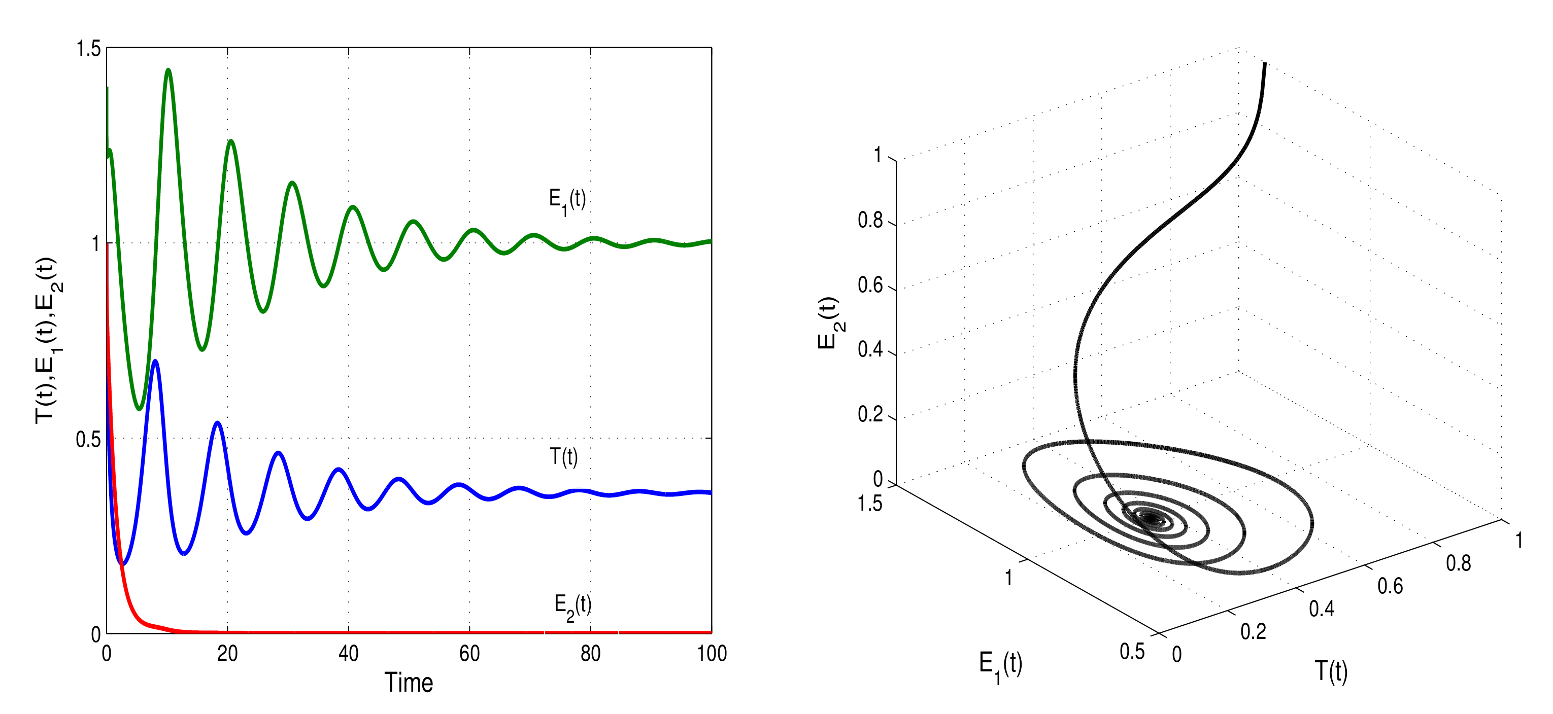
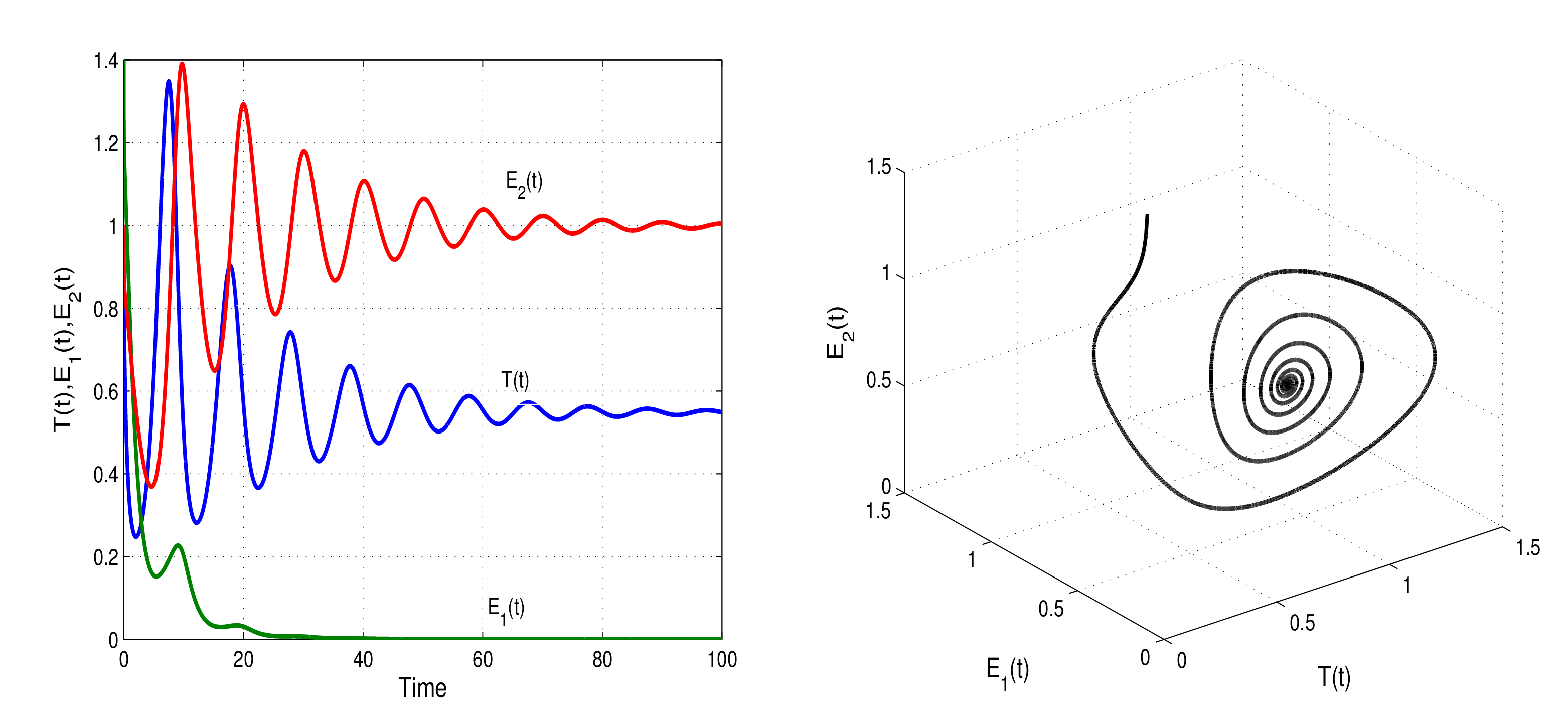
We assign the following parameter values: a = 1 , r 1 = 1 , r 2 = 1 , k 1 = 0.3 , k 2 = 0.7 , d 1 = 0.3 , d 2 = 0.7 .
The deterministic model (1), with long-range temporal memory has endemic steady states, which are locally asymptotically stable, according to conditions (4) and (5): d 1 = 0.3 < 1 , d 2 = 0.7 and d 2 = 0.3 < 1 , d 1 = 0.7 , respectively. Figure 1 and 
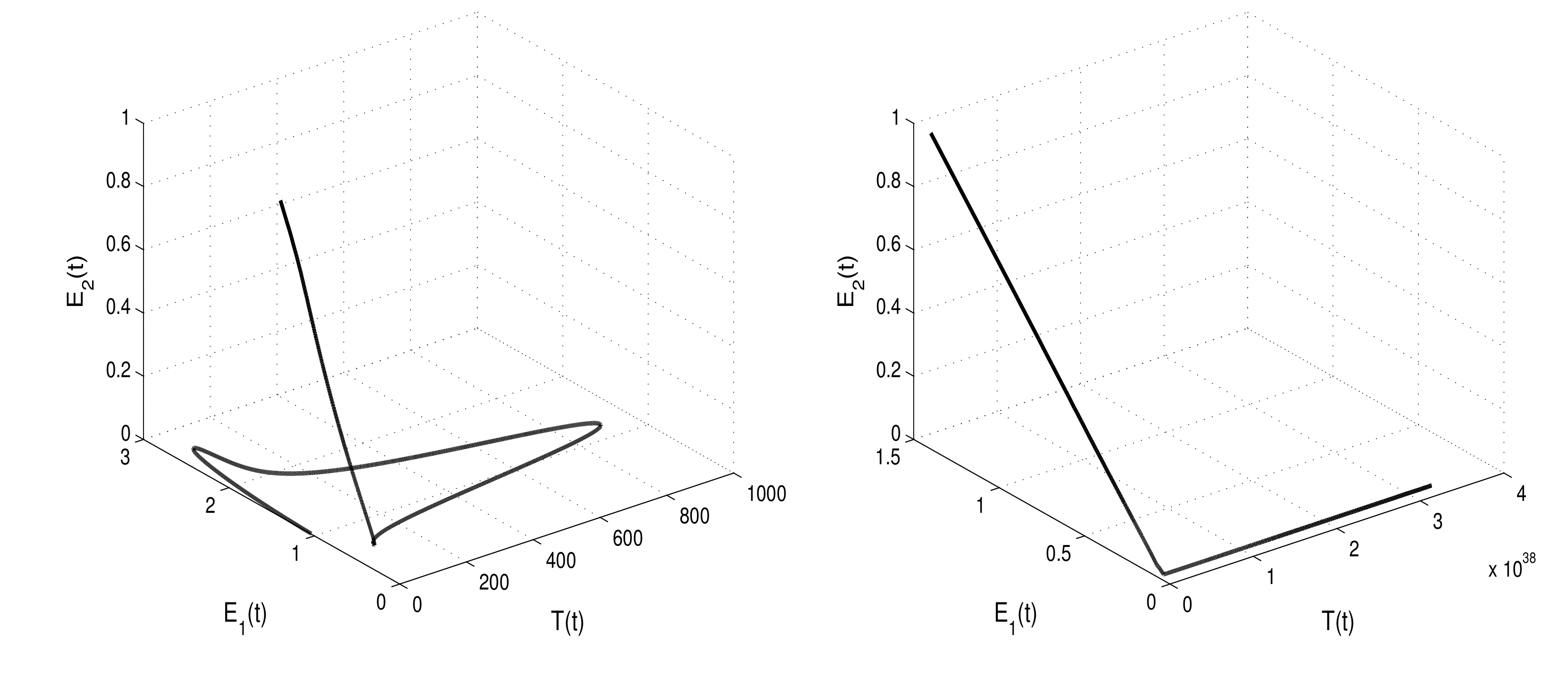
Figure 2 show the numerical simulations of the model with stable memory and endemic steady states. With two cases of parameter values d 1 = d 2 = 0.92 < 1 and d 1 = d 2 = 1.02 > 1 , the stability and instability conditions of model (1) are presented in Figure 3.
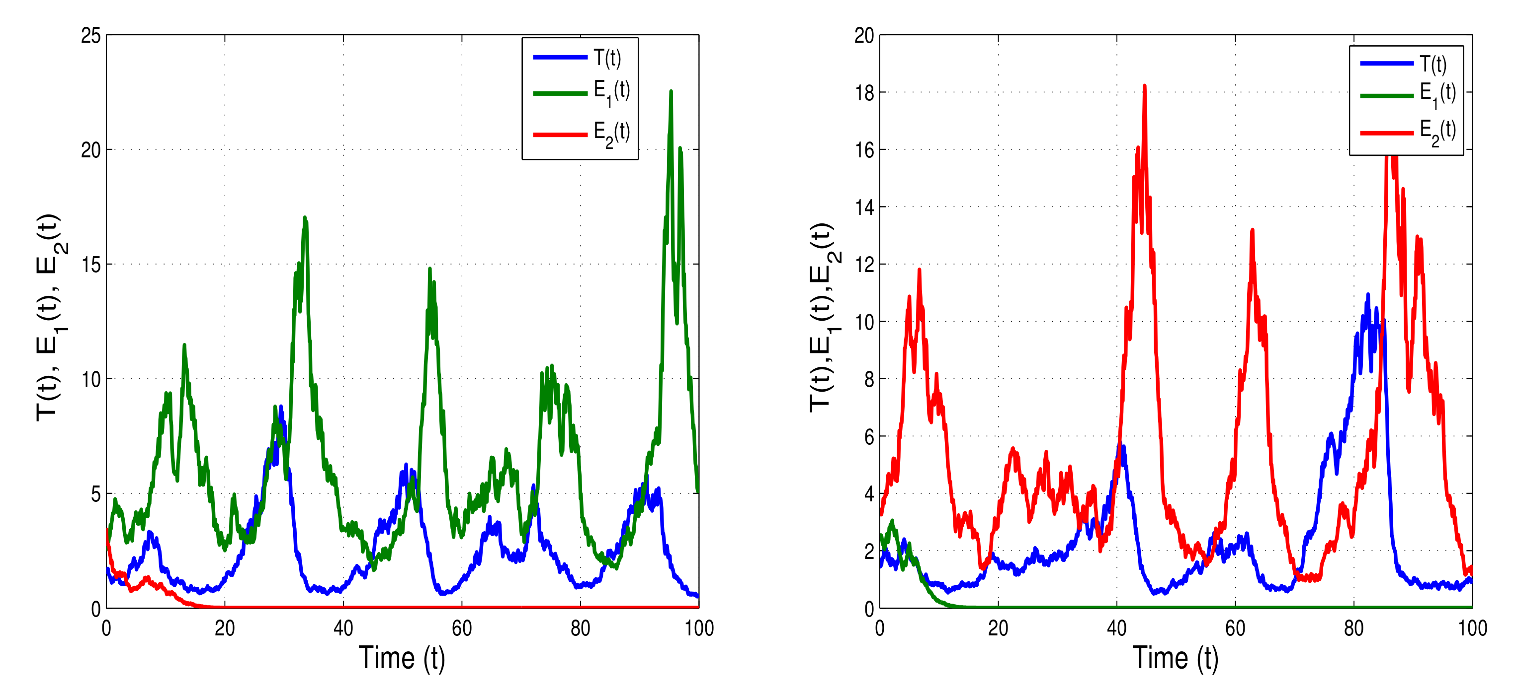
Now, we incorporate white noise in the model to show the dynamics of the stochastic model (6). Initially, we consider the white noise values σ 1 = 0.5 , σ 2 = 0.6 , σ 3 = 0.8 , k 1 = 0.3 , k 2 = 0.7 , d 1 = 0.3 , d 2 = 0.7 (right banner of Figure 4) and k 1 = 0.7 , k 2 = 0.3 , d 1 = 0.7 , d 2 = 0.3 (left banner of Figure 4); the threshold conditions of unique stationary distribution d σ 1 2 σ 2 2 σ 3 2 2 = 0.075 > 0 are satisfied. The left and right banners of Figure 4 show that the tumor cells T ( t ) , effector cells E 1 ( t ) and E 2 ( t ) 
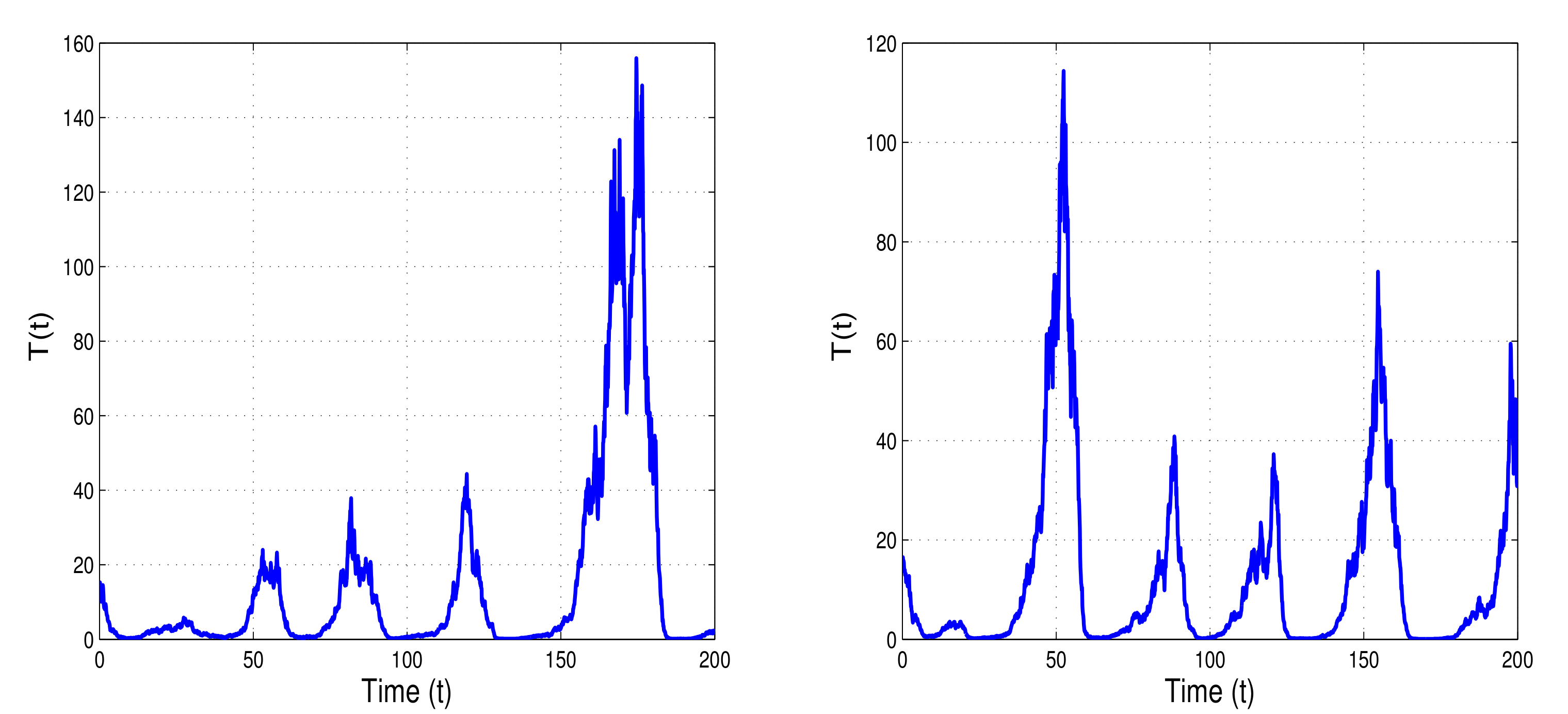
fluctuate randomly. We then slightly increase the white noise values: σ 1 = 0.9 , σ 2 = 1.1 , σ 3 = 1.3 , k 1 = 0.3 , k 2 = 0.7 , d 1 = 0.3 , d 2 = 0.7 (right banner of Figure 5) and k 1 = 0.7 , k 2 = 0.3 , d 1 = 0.7 , d 2 = 0.3 (left banner of Figure 5). When the condition of weak persistence a σ 1 2 2 = 0.595 > 0 is satisfied, we can see in the left and right banners of Figure 5 a weak persistence in the mean of T ( t ) . Tumor cell load T ( t ) gradually decreases and fluctuates in the neighborhood of zero, defining weak persistence in the mean. The intensities of white noise can reduce the certain degree of cancer cells and suppress tumor growth, but not completely eliminate the cancer cells. Thus, the mutation and diffusion of tumor cells can be controlled by varying the strength of noise.
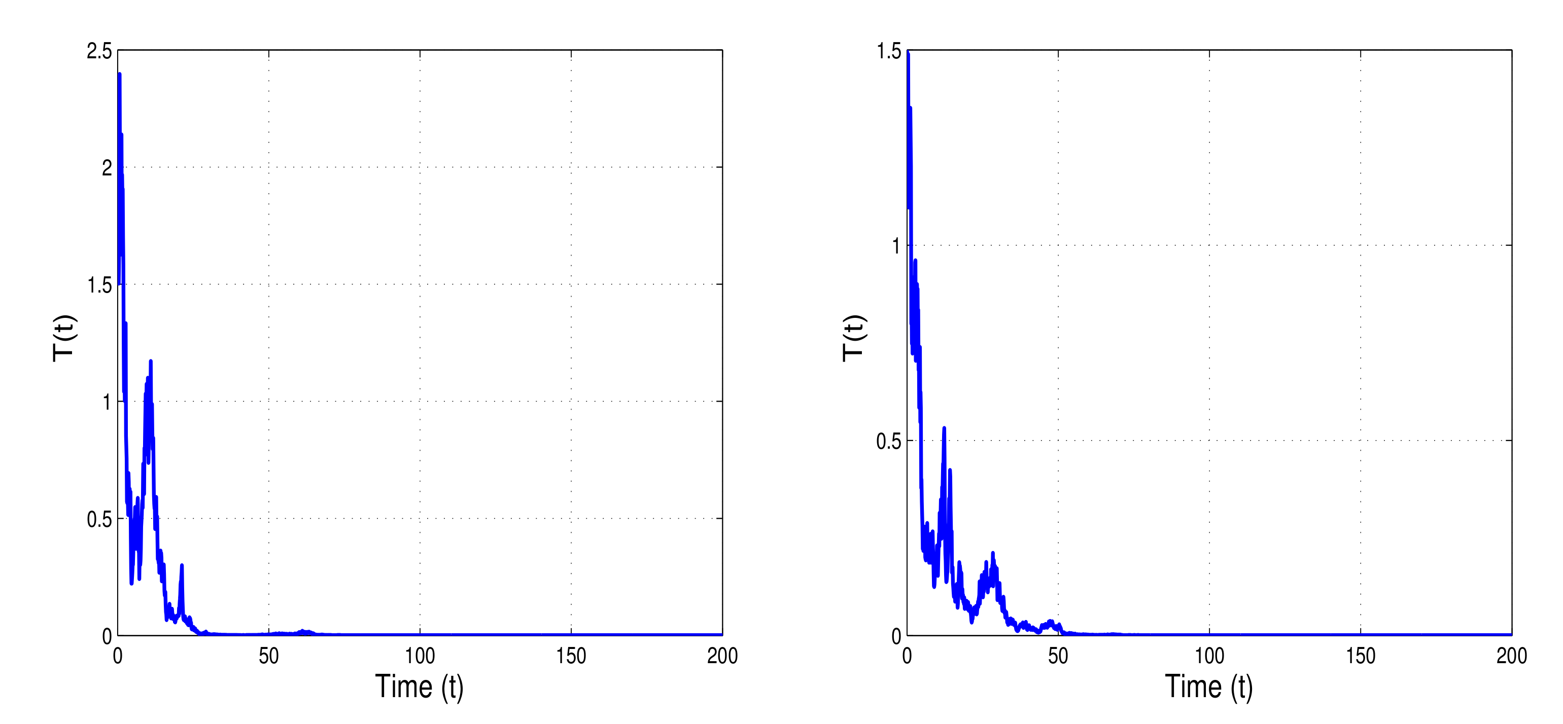
By increasing the white noise values σ 1 = 1.5 , σ 2 = 1.6 , σ 3 = 1.8 , k 1 = 0.3 , k 2 = 0.7 , d 1 = 0.3 , d 2 = 0.7 (right banner of Figure 6) and k 1 = 0.7 , k 2 = 0.3 , d 1 = 0.7 , d 2 = 0.3 (left banner of Figure 6), the condition of extinction results in Theorem 3 a σ 1 2 2 = 0.125 < 0 is satisfied. Figure 6 shows that the tumor cells T ( t ) can die out if the white noise value increases. This serves as evidence that the intensity of environmental noise plays an important role to accelerate tumor extinction.
Remark 4.
As compared to Figure 4, Figure 5 and Figure 6, white noise perturbations on growth and destruction rates promote the elimination of tumor cells T ( t ) . However, increasing the white noise values alters the intra-specific competition rate, which affects the persistence–extinction properties of tumor cells.

6. Conclusions

As enzymatic reactions of proteins are sensitive to environmental changes in the bio-chemical system, in the present paper, we incorporated the noise effect into a tumor-immune model with Holling type III response functions to discuss the fluctuations in cell dynamics. We investigated the existence of global non-negative solutions to such a model. We derived sufficient conditions for unique stationary distribution/stochastic persistence, extinction, and weak persistence of tumor cells, using Ito’s formula and the Lyapunov function. As a result of the stochastic tumor immune model, the following theoretical conditions are obtained:
(i)
If d σ 1 2 σ 2 2 σ 3 2 2 > 0 , then the tumor cells T ( t ) are stochastic persistent and permanent in the tissue a.s.
(ii)
If a > σ 1 2 2 , then T ( t ) shows weak persistence/non-persistence in the mean a.s.
(iii)
If a < σ 1 2 2 , then the tumor cells T ( t ) are eradicated/eliminated a.s.
The numerical simulations are verified based on these sufficient conditions. Furthermore, theoretical and numerical analyses show that the intensity of the noise effect is a prominent factor in controlling and suppressing tumor cell growth in the presence of immune effectors. Dynamical behavior in deterministic and stochastic tumor-immune models is useful to an oncologist and treatment protocols. Treatment protocols can be adapted to cancer patients with the help of environmental fluctuations for better outcomes during public interventions.
Stochastic epidemic models with Markovian switching and time delays are the focus of our future research.

Author Contributions

Data curation, C.R.; Formal analysis, F.A.R. and C.R.; Funding acquisition, F.A.R.; Methodology, F.A.R.; Software, F.A.R. and C.R. All authors have read and agreed to the published version of the manuscript.

Funding

This research was funded by UAE University, fund # 12S005-UPAR 2020.

Data Availability Statement

Not applicable.

Acknowledgments

The authors wish to thank the reviewers and editor for their valuable comments.

Conflicts of Interest

The authors declare no conflict of interest.

References

  1. Mallet, D.G.; Pillis, L.G.D. A cellular automata model of tumor-immune system interactions. J. Theor. Biol. 2006, 239, 334–350. [Google Scholar] [CrossRef] [PubMed] [Green Version]
  2. Nastoupil, L.J.; Rose, A.C.; Flowers, C.R. Diffuse large B-cell lymphoma: Current treatment approaches. Oncology 2012, 26, 488–495. [Google Scholar] [PubMed]
  3. Baskar, R.; Lee, K.A.; Yeo, R.; Yeoh, K.W. Cancer and radiation therapy: Current advances and future directions. Int. J. Med. Sci. 2012, 9, 193–202. [Google Scholar] [CrossRef] [Green Version]
  4. Puhalla, S.; Bhattacharya, S.; Davidson, N.E. Hormonal therapy in breast cancer: A model disease for the personalization of cancer care. Mol. Oncol. 2012, 6, 222–236. [Google Scholar] [CrossRef] [PubMed] [Green Version]
  5. Rihan, F.A.; Velmurugan, G. Dynamics of fractional-order delay differential model for tumor-immune system. Chaos Solitons Fractals 2020, 132, 109592. [Google Scholar] [CrossRef]
  6. Rihan, F.A.; Lakshmanan, S.; Maurer, H. Optimal Control of Tumour-Immune Model with Time-Delay and Immuno-Chemotherapy. Appl. Math. Comput. 2019, 353, 147–165. [Google Scholar] [CrossRef]
  7. Khajanchia, S.; Banerjee, S. Influence of multiple delays in brain tumor and immune system interaction with T11 target structure as a potent stimulator. Math. Biosci. 2018, 302, 116–130. [Google Scholar] [CrossRef]
  8. Adam, J.; Bellomo, N. A Survey of Models for Tumor-Immune System Dynamics; Springer: Berlin/Heidelberg, Germany, 2012. [Google Scholar]
  9. Sharma, S.; Samanta, G. Analysis of the dynamics of a tumor-immune system with chemotherapy and immunotherapy and quadratic optimal control. Differ. Equ. Dyn. Syst. 2016, 24, 149–171. [Google Scholar] [CrossRef]
  10. Tuong, T.D.; Nguyen, N.N.; Yin, G. Longtime behavior of a class of stochastic tumor-immune systems. Syst. Control Lett. 2020, 146, 104806. [Google Scholar] [CrossRef]
  11. Wang, J.; Wang, H. Stochastic effects of the tumor-T cell immune model. Math. Meth. Appl. Sci. 2021, 44, 7228–7237. [Google Scholar] [CrossRef]
  12. Liu, X.; Li, Q.; Pan, J. A deterministic and stochastic model for the system dynamics of tumor-immune responses to chemotherapy. Physica A 2018, 500, 162–176. [Google Scholar] [CrossRef] [Green Version]
  13. Yang, H.; Tan, Y.; Yang, J.; Liu, Z. Extinction and persistence of a tumor-immune model with white noise and pulsed comprehensive therapy. Math. Comput. Simul. 2021, 182, 456–470. [Google Scholar] [CrossRef]
  14. Das, P.D.; Mukherjee, S. Stochastic dynamics of Michaelis-Menten kinetics based tumor-immune interactions. Physica A 2020, 541, 123603. [Google Scholar] [CrossRef]
  15. Li, D.; Cheng, F. Threshold for extinction and survival in stochastic tumor-immune system. Commun. Nonlinear Sci. Numer. Simulat. 2017, 51, 1–12. [Google Scholar] [CrossRef]
  16. Mao, X. Stochastic Differential Equations and Their Applications; Horwood: Chichester, UK, 1997. [Google Scholar]
  17. Mao, X.; Wei, F.; Wiriyakraikul, T. Positivity preserving truncated Euler–Maruyama Method for stochastic Lotka–Volterra competition model. J. Comput. Appl. Math. 2021, 394, 113566. [Google Scholar] [CrossRef]
  18. Cai, S.; Cai, Y.; Mao, X. A stochastic differential equation SIS epidemic model with regime switching. Discret. Contin. Dyn. Syst. B 2021, 26, 4887. [Google Scholar] [CrossRef]
  19. Rihan, F.A. Delay Differential Equations and Applications to Biology; Springer: Singapore, 2021. [Google Scholar] [CrossRef]
  20. Kirschner, D.; Panetta, J. Modeling immunotherapy of the tumor-immune interaction. J. Math. Biol. 1998, 37, 23–52. [Google Scholar] [CrossRef] [PubMed] [Green Version]
  21. Anderson, A.; Maini, P. Mathematical Oncology. Bull. Math. Biol. 2018, 80, 945–953. [Google Scholar] [CrossRef] [Green Version]
  22. Chaplain, M. Multiscale mathematical modelling in biology and medicine. IMA J. Appl. Math. 2011, 76, 371–388. [Google Scholar] [CrossRef] [Green Version]
  23. de Pillis, L.; Radunskaya, A. A Mathematical Model of Immune Response to Tumor Invasion A2—Bathe KJ Computational Fluid and Solid Mechanics; Elsevier: Amsterdam, The Netherlands, 2003. [Google Scholar]
  24. de Pillis, L.; Radunskaya, A.; Wiseman, C. A Validated Mathematical Model of Cell-Mediated Immune Response to Tumor Growth. Cancer Res. 2005, 65, 7950–7958. [Google Scholar] [CrossRef] [Green Version]
  25. Rihan, F.; Abdelrahman, D.; Lakshmanan, S. A Time Delay Model of Tumour-Immune System Interactions: Global dynamics, Parameter estimation, Sensitivity analysis. Appl. Math. Comput. 2014, 232, 606–623. [Google Scholar] [CrossRef]
  26. Luzyanina, T.; Bocharov, G. Stochastic modeling of the impact of random forcing on persistent hepatitis B virus infection. Math. Comput. Simul. 2014, 96, 54–65. [Google Scholar] [CrossRef]
  27. Kiouach, D.; Sabbar, Y. Ergodic Stationary Distribution of a Stochastic Hepatitis B Epidemic Model with Interval-Valued Parameters and Compensated Poisson Process. Comput. Math. Methods Med. 2020, 2020, 9676501. [Google Scholar] [CrossRef] [PubMed]
  28. Zhang, X.; Peng, H. Stationary distribution of a stochastic cholera epidemic model with vaccination under regime switching. Appl. Math. Lett. 2020, 102, 106095. [Google Scholar] [CrossRef]
  29. Rihan, F.A.; Alsakaji, H.J.; Rajivganthi, C. Stochastic SIRC epidemic model with time-delay for COVID-19. Adv. Differ. Equ. 2020, 2020, 1–20. [Google Scholar] [CrossRef]
  30. ksendal, B. Stochastic Differential Equations: An Introduction with Applications, 6th ed.; Springer: New York, NY, USA, 2003. [Google Scholar]
  31. Liu, Q.; Jiang, D.; Hayat, T.; Alsaedi, A. Dynamics of a stochastic tuberculosis model with antibiotic resistance. Chaos Solitons Fractals 2018, 109, 223–230. [Google Scholar] [CrossRef]
  32. Hasminskii, R.Z. Stochastic Stability of Differential Equations; Springer Science & Business Media: Amsterdam, The Netherlands, 2012; p. 1980. [Google Scholar]
  33. Higham, D.J. An algorithmic introduction to numerical simulation of stochastic differential equations. SIAM Rev. 2001, 43, 525–546. [Google Scholar] [CrossRef]
Figure 1. Left banner shows the numerical solutions of the deterministic model (1) when the conditions given in (4) are satisfied ( a = 1 , r 1 = r 2 = 1 , k 1 = 0.3 , k 2 = 0.7 , d 1 = 0.3 < d 2 = 0.7 and d 1 < 1 ). Right (top and bottom banners): the relation between the tumor cells and effector cells E 1 ( t ) , E 2 ( t ) . The system converges to a stable steady state.
Mathematics 09 02707 g001
Figure 2. Left banner displays the numerical simulations of the deterministic model (1) when the conditions given in (5) are satisfied ( a = 1 , r 1 = r 2 = 1 , k 1 = 0.7 , k 2 = 0.3 , d 1 = 0.7 > d 2 = 0.3 and d 2 < 1 ). Right (top and bottom banners): the relation between the tumor cells T ( t ) and effector cells E 1 ( t ) , E 2 ( t ) . The endemic state is locally asymptotically stable.
Mathematics 09 02707 g002
Figure 3. Shows the stability (left) of the solution of the deterministic system (1) when d 1 = 0.92 = d 2 < 1 and instability (right) of the solution when d 1 = d 2 = 1.02 > 1 .
Mathematics 09 02707 g003
Figure 4. Shows time trajectories for tumor cells T ( t ) , and effector cells E 1 ( t ) , E 2 ( t ) of the stochastic model (6) with k 1 = 0.7 , k 2 = 0.3 , d 1 = 0.7 , d 2 = 0.3 (right banner) and k 1 = 0.3 , k 2 = 0.7 , d 1 = 0.3 , d 2 = 0.7 (left banner) and d σ 1 2 σ 2 2 σ 3 2 2 = 0.075 > 0 . The threshold conditions of unique stationary distribution is satisfied based on Theorem 2.
Mathematics 09 02707 g004
Figure 5. Shows time trajectories for tumor cell T ( t ) of the stochastic model (6) with k 1 = 0.7 , k 2 = 0.3 , d 1 = 0.7 , d 2 = 0.3 (right banner) and k 1 = 0.3 , k 2 = 0.7 , d 1 = 0.3 , d 2 = 0.7 (left banner) and a σ 1 2 2 = 0.595 > 0 . The weak persistence condition is satisfied under Remark 1.
Mathematics 09 02707 g005
Figure 6. Shows time trajectories for tumor cells T ( t ) of the stochastic model (6) with k 1 = 0.7 , k 2 = 0.3 , d 1 = 0.7 , d 2 = 0.3 (right banner) and k 1 = 0.3 , k 2 = 0.7 , d 1 = 0.3 , d 2 = 0.7 (left banner) and a σ 1 2 2 = 0.125 < 0 . The threshold conditions of extinction is verified based on Theorem 3. In it, stochastic noise is shown to suppress the explosion of population T(t).
Mathematics 09 02707 g006
Publisher’s Note: MDPI stays neutral with regard to jurisdictional claims in published maps and institutional affiliations.

