Abstract
Since correlated stochastic processes are often presented in practical problems, feasible methods to model and generate correlated processes appropriately are needed for analysis and simulation. The present paper systematically presents three methods to generate two correlated stationary Gaussian processes. They are (1) the method of linear filters, (2) the method of series expansion with random amplitudes, and (3) the method of series expansion with random phases. All three methods intend to match the power spectral density for each process but use information of different levels of correlation. The advantages and disadvantages of each method are discussed.
1. Introduction
Stochastic processes are involved in many areas, such as physics, engineering, ecology, biology, medicine, psychology, finance, and other disciplines. For purposes of analysis and simulation, they are required to be properly modeled and generated mathematically, according to their measured or estimated statistical and probabilistic properties. Among various properties, the probability distribution and the power spectral density are the most important. If it is stationary, both properties are invariant with time. Based on these two properties, several methods were developed to model a single stationary process. If it is Gaussian, a process with a given spectral density can be generated [1,2]. If a process is non-Gaussian, methods were proposed for processes defined in an infinite region, a semi-infinite region, or a finite region [2]. In this case, only certain types of spectral density functions can be matched, such as low-pass spectrum, single-peak spectrum, and two-peak spectrum.
In some problems, two stochastic processes are present and play roles in system dynamics. If they are correlated, the above-mentioned modeling methods for single processes are incomplete. The correlation of the two processes should be taken into account. A typical scenario is structure vibration caused by earthquakes. In general, the ground motion in an earthquake has both horizontal and vertical components. Both may play roles in the destruction of structures. One example is the vibration of a water tank supported by a column and subjected to both horizontal and vertical ground motions [3]. Since both motions are in fact the two components of the same ground motion, they must be correlated, not independent. Another typical situation is the ship rolling motion caused by random sea waves, investigated in [4,5]. In the equation of the motion of the ship rolling angle, there are two excitation terms, an external excitation representing the moment changing the rolling angle directly and a parametric excitation caused by the wave level relative to the rolling ship. The two excitations by the same sea waves are naturally correlated.
It is a common practice that many stochastic processes are assumed to be Gaussian, except cases with obvious non-Gaussian distributions. Several reasons support such a practice, including that (i) the bell shape of the Gaussian distribution matches many real processes; (ii) its mathematical treatment is simple; (iii) the Gaussian distribution is commonly used for temporal and spectral smoothing in a time-frequency analysis [6]; and (iv) the generation of a stochastic process with a given non-Gaussian distribution and a given spectral density is much more difficult [7,8,9]. Moreover, the power spectral density describes the energy distribution of the process in the frequency domain, and it is more important than the probability distribution in many situations [10]. Therefore, the Gaussian distribution is usually assumed, and the spectral density is used to generate an individual process. In this investigation, the emphasis is on the correlation of the two processes.
It is known that the correlation of two stochastic processes can be described at different levels, such as their joint moment or correlation coefficient, their cross-correlation function, or their cross-spectral density. To model and generate two correlated stationary stochastic processes, various methods were developed, such as the methods using series expansions [11,12,13], based on an autoregressive moving average model [14,15], using linear filters [16], and based on other methods [17,18]. The present paper is a review paper, summarizing three relatively simple and practical methods to model and generate two correlated stationary Gaussian processes based on different levels of their correlation information. They are the method of linear filters, the method of series expansion with random amplitudes, and the method of series expansion with random phases. The three methods are presented systematically, and simulations are performed to verify their accuracy. The relative advantages and disadvantages of each method are pointed out for the convenience of practical applications.
2. Method of Linear Filters
2.1. Two Correlated Gaussian White Noises
Gaussian white noises are the most commonly used stochastic processes in various fields of science and technology due to the simplicity in mathematical treatment and the relation to the Markov theory. For example, white noises are frequently used for simulations in signal processing since many real-world signals contain white noises. Moreover, they can be used to generate more realistic stochastic processes [2]. Thus, we would develop a method to model two correlated Gaussian white noises W1(t) and W2(t). Assume that they have the following correlation functions:
where K11 and K22 are the spectral densities of W1(t) and W2(t), respectively; K12 is their cross-spectral density, which is the unique measure of their correlation. The samples of W1(t) and W2(t) can be generated as follows:
where Δt is a small time interval; X1k and X2k are samples of two Gaussian random variables with a correlation coefficient
The procedure of generating X1k and X2k is described in reference [2]. It is noted that each of the X1k and X2k sequences is independent for different k values, and X1i and X2j are independent for i ≠ j. It is proved that the spectral densities of X1k and X2k are [2]
and their cross-spectral density is [2]
In the limiting process ωΔt → ∞, we have
Equations (6) and (7) show that if is very small, the spectral densities are approximately constants matching the given values. Therefore, the time step Δt is the most important parameter in the simulation, and a smaller Δt leads to broader frequency bands for both noises. It is pointed out that Δt should be much shorter than all important system relaxation times [2].
2.2. Two Correlated Gaussian Processes
It is known that the response of a linear filter excited by a Gaussian white noise is also Gaussian, but its spectrum may have different shapes. A first-order filter generates a process of low-pass spectrum, i.e., its peak is at zero frequency. A second-order filter has a response of a single-peak spectrum with its peak at a non-zero frequency. The response of a higher-order filter has a spectrum of multiple peaks. Moreover, the bandwidth of each peak can be adjusted by appropriately selecting the filter parameters. In the following, an example of two correlated stochastic processes, one of low-pass and another of single peak at non-zero frequency, is given for illustration.
Consider the system consisting of one first-order filter and one second-order filter, described by
where W1(t) and W2(t) are two correlated Gaussian white noises with the spectral densities K11 and K11, and the cross-spectral density K12. Letting , Equation (8) is re-written in the state space as
Equation (9) generates three stochastic processes, X1(t), X2(t), and X3(t). Since X3(t) is the derivative of X2(t), they are uncorrelated; thus, the two pairs of correlated processes are X1(t) and X2(t), and X1(t) and X3(t).
The auto- and cross-correlation functions can be determined exactly following the method described in [2]. The autocorrelation functions are found to be
and the cross-correlations are
where
and
For the negative range of τ < 0, it is known that and .
Equations (11) and (12) show that the correlation function of X1(t) and X2(t) is specified by the joint moment E[X1 × 2], and that of X1(t) and X3(t) by E[X1X3]. Both joint moments are determined by K12, as shown in the last equation in (14). Thus, the correlation level of either X1(t) and X2(t) or X1(t) and X3(t) can be matched by adjusting K12.
It is noted that X3(t) has been used to generate the random wave excitation in the ship rolling motion [19,20].
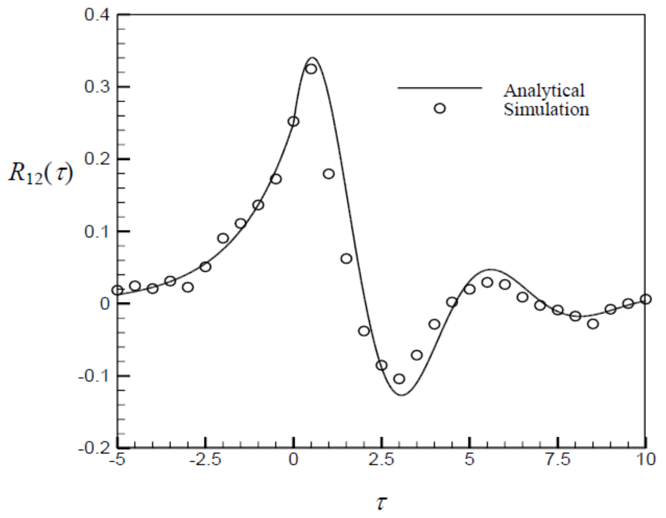
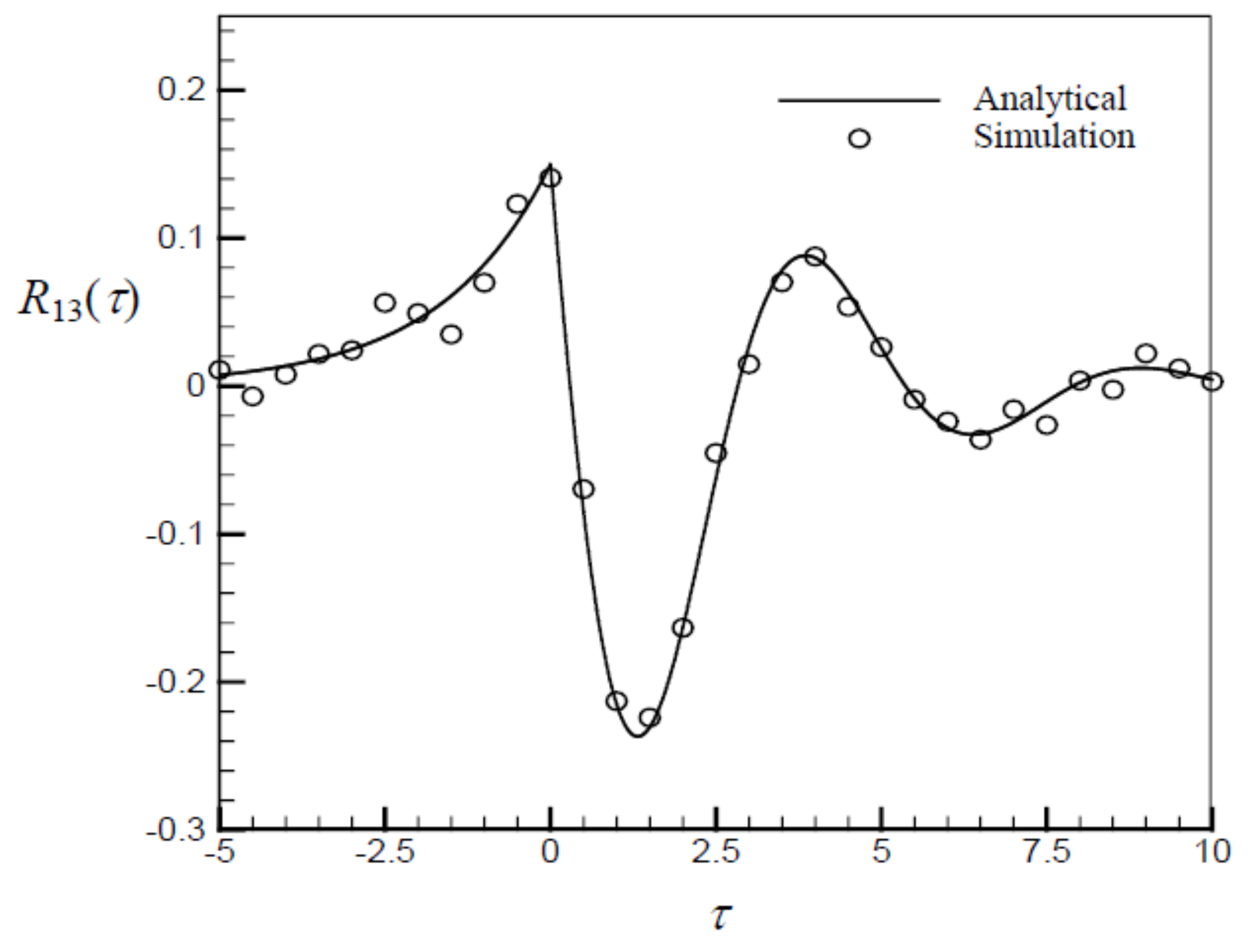
The cross-correlation functions R12(τ) and R13(τ) are calculated from Equations (11) and (12) and depicted in Figure 1 and Figure 2 for Equation (9) with parameter values of α = 0.6, ζ = 0.3, = 1.3, K11 = 1, K22 = 0.5, and K12 = 0.1. The results from Monte Carlo simulations are also shown in the figures. They agree quite well.
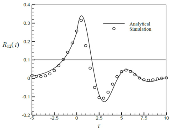
Figure 1.
Cross−correlation function R12(τ) of X1(t) and X2(t) for Equation (9) using the linear filter method.
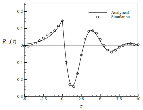
Figure 2.
Cross−correlation function R13(τ) of X1(t) and X3(t) for Equation (9) using the linear filter method.
One advantage of using linear filters is that the generated correlated stochastic processes are ergodic after a short transient period. It is important since only one sample function is needed in the simulation provided that the sample function is long enough.
3. Method of Series Expansion with Random Amplitudes
3.1. Simulation of a Single Stationary Gaussian Process
Assume that a stationary Gaussian process X(t) possesses a power spectral density . For practical situations, → 0 when ω → ∞; therefore, there is a cutting frequency , beyond which is negligible. Moreover, assume that there is a lower frequency band , below which Φ(ω) can also be neglected. In many cases, = 0. Divide into N intervals, and denote
By noting that,
in Equation (15) specifies the contribution of the spectral density in the jth interval toward a total mean-square value of X(t) [2]. Denote Xs(t) with the subscript which represents s as a sample function of X(t). The following series can be used to generate Xs(t),
where each of Uj and Vj is a series of Gaussian random variables independent for different j, and Uj and Vj are also independent for any j, and which are determined from (15).
The correlation function and spectral density of Xs(t) are, respectively, [2]
The summation in (19) becomes an integration when N → ∞ and Δω → 0, i.e.,
indicating that Xs(t) is a good sample function of X(t) if the interval number N is large and the frequency interval Δω is small.
3.2. Generation of Two Correlated Stationary Gaussian Processes
Now we try to model two stationary Gaussian processes X1(t) and X2(t) with power spectral densities Φ11() and Φ22(), respectively. First, we have to determine a common frequency range for both processes and apply Equation (15) for each process. Then, the sample function Xis(t) (i = 1 or 2) of each process can be generated from (17) as follows:
In order to make the two processes correlated, U1j and U2j in (21) are generated with a correlation coefficient ρ, as well as V1j and V2j. It is shown in [13] that
and
Replacing and according to Equation (15),
As Δω → 0 and N → ∞, Equations (22) and (24) are transferred to
Equation (26) indicates that the correlation coefficient of X1 (t) and X2 (t), denoted as ρ12, is obtained as follows
Then, for a given ρ12, ρ can be calculated from (27) and used to generate Uij and Vij in (21).
The advantage of the above method is that the arbitrary spectral densities of the two processes can be matched exactly, and that only the correlation coefficient is needed regarding the correlation information of the two processes. However, the generated processes are not ergodic, and a large number of samples is required in simulations.
The above method was used to model two correlated ocean wave forces on the ship rolling motion. One of the commonly used spectral densities for the ocean wave forces is known as the Pierson–Moskowits spectrum [21] which is used in [5,19,20,22,23,24,25,26,27]. The spectral density is controlled by two parameters, the peak frequency ωp and the mean-square value σ2 specifying the intensity of the process. It is represented by
where the peak value of the spectrum is determined by
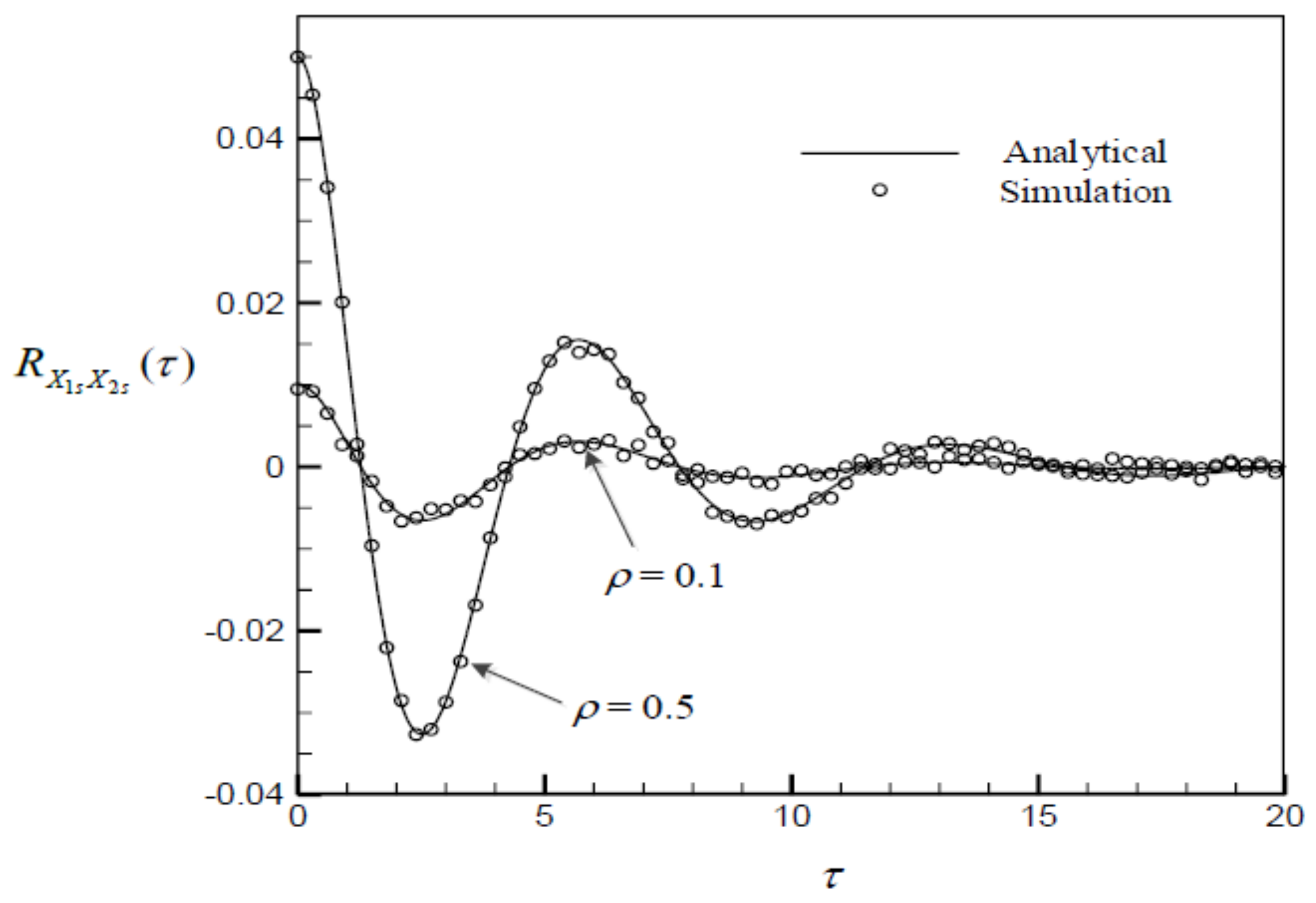
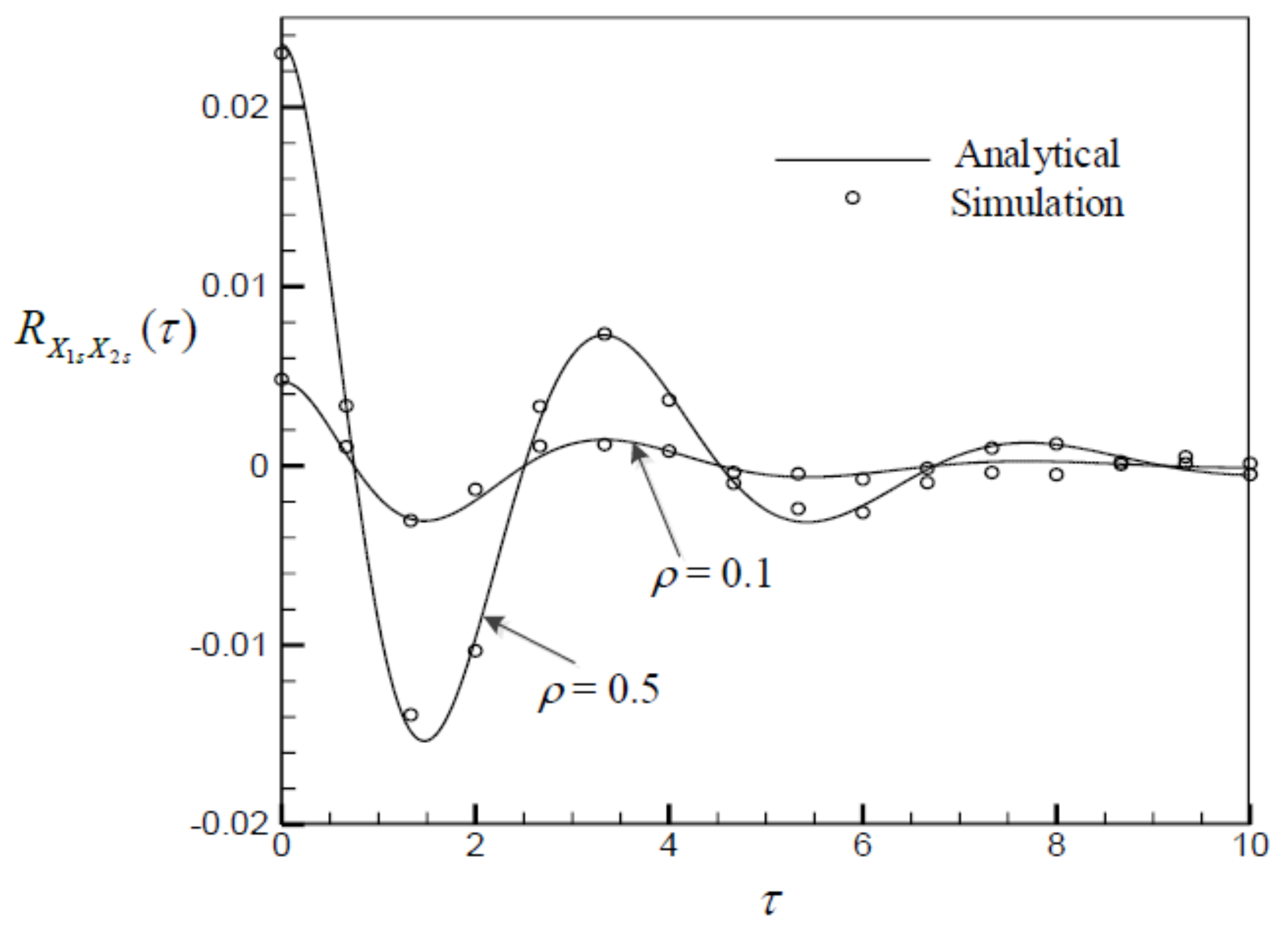
The two correlated ocean wave forces with the Pierson–Moskowits spectrum of a different peak frequency and/or different intensity σ2 can be modeled using the series expansion Equation (17). Some numerical results are shown in Figure 3 for two processes with the same and σ2, and in Figure 4 for those of a different peak and the same σ2. The analytical results are obtained from Equation (25), and the simulation results are calculated from Equation (17).
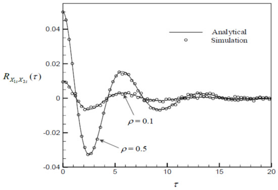
Figure 3.
Cross−correlation functions of simulated excitations for == 0.1, == 1, and different values of ρ.
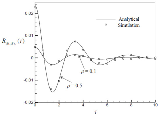
Figure 4.
Cross−correlation functions of simulated excitations for == 0.1, =1, = 2, and different values of ρ.
4. Method of Series Expansion with Random Phases
Simulations of stochastic processes using a series with random phases based on their spectral representations were proposed and developed in [11,12].
4.1. Simulation of a Single Stationary Gaussian Process
A Gaussian process X(t) can be simulated from
where ωj and Δω are determined from Equation (15), and ϕj are independent random variables uniformly distributed in [0, 2π). In each term in Equation (30), represents a random variable for a given t. For different j, these random variables are independent and have an identical probability distribution. According to the central limit theorem, the probability distribution of Xs(t) in (30) converges to a Gaussian distribution as the number of terms N approaches infinity. The correlation function of Xs(t) is obtained as
Equation (31) is the same as Equation (18), and the spectral density of Xs(t) is the same as that given in Equations (19) and (20), respectively.
4.2. Generation of Two Correlated Stationary Gaussian Processes
Assume that the spectral density functions of two correlated stochastic processes X1(t) and X2(t) are given as Φ11(), Φ12(), Φ21(), and Φ22(). In matrix form, we have
It is known that for i, j = 1, 2,
where the asterisk denotes the complex conjugate. Equation (33) indicates that the power spectral density functions are real, nonnegative, and even, and the cross-spectral densities are generally complex, with even real parts and odd imaginary parts. Denote a high triangular matrix H() as
which satisfies
where the superscript T denotes the transpose of the matrix. It is found from (35) that
The two processes can then be simulated from
where and Δ are determined from Equation (15); and are mutually independent random variables uniformly distributed in [0, 2π), and they are also independent for different j, and θ(ω) is determined from , namely,
It is known from Equations (32), (36), and (39) that function θ() is an odd function, i.e.,
Equation (38) has the same form as Equation (30). The correlation function of X1s(t) is obtained as
which has the same form as Equation (31). The cross-correlation functions of X1s(t) and X2s(t) are obtained as
When Δω → 0 and N → ∞, Equation (42) tends to
Since θ() is an odd function, we have
Taking (44) into account, Equation (43) can be rewritten as
In deriving (45), Equations (36) and (39) are used. Equation (45) indicates that the cross-correlation function of the processes given by (37) and (38) approaches that of the target processes.
As an example to illustrate the procedure, take the three processes X1(t), X2(t), and X3(t) in system (9) for numerical calculation. Their cross-correlations R12(τ) and R13(τ) are given in Equations (11) and (12). The spectral densities can be obtained by using the Fourier transform, or by using the method described in [2], as follows:
where E[X1X2] is given in Equation (14), and Δ is given by
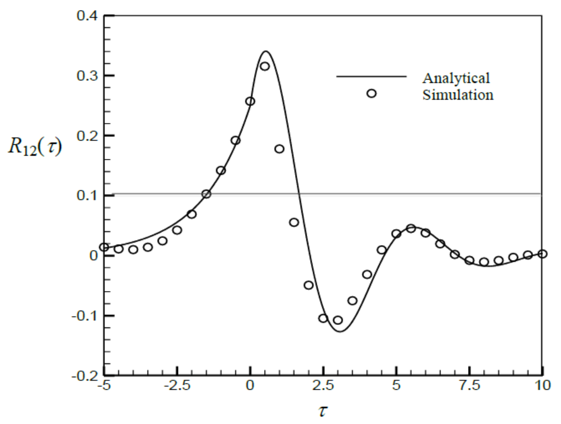
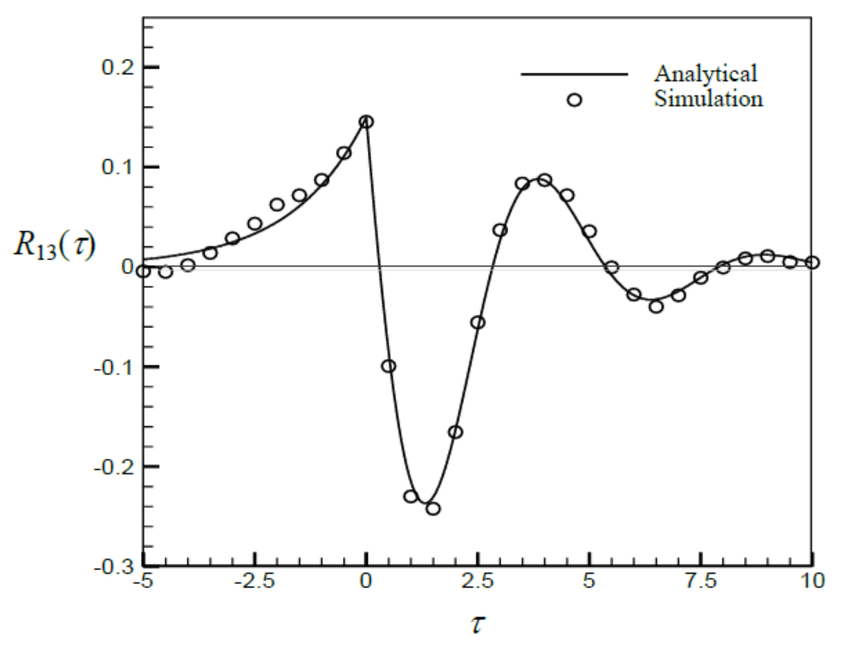
Numerical calculations are carried out for the same parameter values as those used in Figure 1 and Figure 2, i.e., α = 0.6, ζ = 0.3, ω0 = 1.3, K11 = 1, K22 = 0.5, and K12 = 0.1. The cross-correlation functions R12() and R13() are depicted in Figure 5 and Figure 6, respectively. The analytical results are calculated from Equations (11) and (12), and the simulation results are obtained using Equations (37) and (38) with the spectral densities given by Equations (46)–(48).
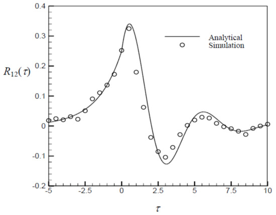
Figure 5.
Cross−correlation function R12(τ) of X1(t) and X2(t) for Equation (9) using the method of series expansion with random phases.
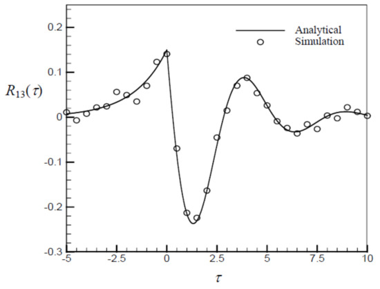
Figure 6.
Cross−correlation function R13(τ) of X1(t) and X3(t) for Equation (9) using the method of series expansion with random phases.
It is clear that the method of the series expansion is the most sophisticated method if the cross-correlation function or the cross-spectral density of the two processes is known. The same disadvantage is presented as that of the method of the series expansion with random amplitudes, specifically, that the generated processes are not ergodic.
5. Conclusions
Three methods to generate two correlated stationary Gaussian processes are reviewed and presented systematically. Their accuracy is substantiated by simulations. The three methods have their own advantages and disadvantages, and they need to be applied in different situations.
The method of linear filters offers a simple way to simulate two processes with a given power spectral density for each process and with their joint moment or correlation coefficient. The generated processes are ergodic after a short period of time. This is a valuable advantage for simulations since only a single sample function is needed for calculation. For low-pass processes and processes of a single spectrum peak, the method is especially feasible by simply using first-order and second-order filters. However, if processes with more complicated shapes of spectra, such as multiple spectrum peaks, higher-order filters are required, and it is more difficult to determine the parameters in the filters.
Similar to the method of linear filters, the method of series expansion with random amplitudes is also based on the power spectra of the two processes and their correlation coefficient. The advantage of the method is the exact match of the power spectral density for each process. However, the modeled stochastic processes are not ergodic, and large numbers of sample functions must be generated for simulations.
The above two methods only use the correlation coefficient of the two correlated processes, which is incomplete information of the correlation. If the correlation function, as the complete information of the correlation of the two processes, is known, the method of series expansion with random phases is the most accurate. It generates the two processes with exactly matched power spectral densities and cross-spectral density. Similar to the series expansion method with random magnitudes, the generated processes are not ergodic for an arbitrary length of time period even it is very long.
In practical problems, the correlation function may not be known, and only the extent of the correlation can be estimated; thus, the first two methods are more feasible.
Author Contributions
All authors have participated in writing, review, and editing. All authors have read and agreed to the published version of the manuscript.
Funding
This work is partially supported by the National Natural Science Foundation of China under grants No. 11772293 and No. 12172323.
Institutional Review Board Statement
Not applicable.
Informed Consent Statement
Not applicable.
Data Availability Statement
Not applicable.
Conflicts of Interest
The authors declare no conflict of interest.
References
- Shinozuka, M.; Deodatis, G. Simulation of stochastic processes by spectral representation. Appl. Mech. Rev. 1991, 44, 191–204. [Google Scholar] [CrossRef]
- Cai, G.Q.; Zhu, W.Q. Elements of Stochastic Dynamics; World Scientific Publisher: Singapore, 2016. [Google Scholar]
- Lin, Y.K.; Cai, G.Q. Probabilistic Structural Dynamics. In Advanced Theory and Applications; McGraw-Hill: New York, NY, USA, 1995, 2004. [Google Scholar]
- Muhuri, P.K. A study of the stability of the rolling motion of a ship in an irregular seaway. Int. Shipbuild. Prog. 1980, 27, 139–142. [Google Scholar] [CrossRef]
- Roberts, J.B. A stochastic theory for nonlinear ship rolling in irregular seas. J. Ship Res. 1982, 26, 229–245. [Google Scholar] [CrossRef]
- Ghaderpour, E.; Pagiatakis, S.D. Least-squares wavelet analysis of unequally spaced and non-stationary time series and its applications. Mathematical Geosci. 2017, 49, 819–844. [Google Scholar] [CrossRef]
- Winterstein, S.R. Nonlinear vibration models for extremes and fatigue. J. Eng. Mech. 1988, 114, 1772–1790. [Google Scholar] [CrossRef]
- Grigoriu, M. Simulation of stationary non-Gaussian translation processes. J. Eng. Mech. 1998, 124, 121–126. [Google Scholar] [CrossRef]
- Deodatis, G.; Micaletti, R.C. Simulation of highly skewed non-Gaussian stochastic processes. J. Eng. Mech. 2001, 127, 1284–1295. [Google Scholar] [CrossRef]
- Wu, C.; Cai, G.Q. Effects of excitation probability distribution on system responses. Int. J. Non-Linear Mech. 2004, 39, 1463–1472. [Google Scholar] [CrossRef]
- Shinozuka, M.; Jan, C.M. Digital simulation of random processes and its applications. J. Sound Vib. 1972, 25, 111–128. [Google Scholar] [CrossRef]
- Deodatis, G. Simulation of ergodic multivariate stochastic processes. J. Eng. Mech. 1996, 122, 778–787. [Google Scholar] [CrossRef]
- Cai, G.Q.; Zhu, W.Q. Generation of two correlated stationary Gaussian processes and application to ship rolling motion. Probabilistic Eng. Mech. 2019, 57, 26–31. [Google Scholar] [CrossRef]
- Mignolet, M.P.; Spanos, P.D. Recursive simulation of stationary multi-variate random processes, Part, I. J. Appl. Mech. 1987, 54, 674–680. [Google Scholar] [CrossRef]
- Mignolet, M.P.; Spanos, P.D. Recursive simulation of stationary multi-variate random processes, Part II. J. Appl. Mech. 1987, 54, 681–687. [Google Scholar] [CrossRef]
- Cai, G.Q. Generation of correlated random variables and stochastic processes. Probab. Eng. Mech. 2018, 52, 40–46. [Google Scholar] [CrossRef]
- Li, Y.; Kareem, Q. Simulation of multi-variate random processes, hybrid DFT and digital filtering approach. J. Eng. Mech. 1993, 119, 1078–1098. [Google Scholar] [CrossRef]
- Ramadan, O.; Novak, M. Simulation of spatially incoherent random ground motions. J. Eng. Mech. 1993, 119, 997–1016. [Google Scholar] [CrossRef]
- Chai, W.; Naess, A.; Leira, B.J. Filter models for prediction of stochastic ship roll response. Probab. Eng. Mech. 2015, 41, 104–114. [Google Scholar] [CrossRef]
- Chai, W.; Naess, A.; Leira, B.J. Stochastic nonlinear ship rolling in random beam seas by path integration method. Probabilistic Eng. Mech. 2016, 44, 43–52. [Google Scholar] [CrossRef]
- Pierson, W.J.; Moskowitz, L.A. A proposal spectral form for fully developed wind seas based on the similarity theory of S. A. Kitaigorodskii. J. Geophys. Res. 1964, 69, 5181–5190. [Google Scholar] [CrossRef]
- Dalzell, J.F. A Study of the Distribution of Maxima of Non-Linear Ship Rolling in a Seaway; Report DL-71-1562; Stevens Institute of Technology: Hoboken, NJ, USA, 1971. [Google Scholar]
- Dalzell, J.F. A Note on the distribution of maxima of ship rolling. J. Ship Res. 1973, 17, 217–226. [Google Scholar] [CrossRef]
- Faltinsen, O.M. Sea Loads on Ships and Offshore Structures; Cambridge University Press: Oxford, UK, 1993. [Google Scholar]
- Hsieh, S.R.; Troesch, A.W.; Shaw, S.W. A nonlinear probabilistic method for predicting vessel capsizing in random beam seas. Proc. R. Soc. Lond. A 1994, 446, 195–211. [Google Scholar]
- Paroka, D.; Ohkura, Y.; Umeda, N. Analytical prediction of capsizing probability of a ship in beam wind and waves. J. Ship Res. 2006, 50, 187–195. [Google Scholar] [CrossRef]
- Kougioumtzoglou, I.A.; Spanos, P.D. Stochastic response analysis of the softening Duffing oscillator and ship capsizing probability determination via a numerical path integral approach. Probab. Eng. Mech. 2014, 35, 67–74. [Google Scholar] [CrossRef]
Publisher’s Note: MDPI stays neutral with regard to jurisdictional claims in published maps and institutional affiliations. |
© 2021 by the authors. Licensee MDPI, Basel, Switzerland. This article is an open access article distributed under the terms and conditions of the Creative Commons Attribution (CC BY) license (https://creativecommons.org/licenses/by/4.0/).