Outer Approximation Method for the Unit Commitment Problem with Wind Curtailment and Pollutant Emission

Abstract

This paper considers the fast and effective solving method for the unit commitment (UC) problem with wind curtailment and pollutant emission in power systems. Firstly, a suitable mixed-integer quadratic programming (MIQP) model of the corresponding UC problem is presented by some linearization techniques, which is difficult to solve directly. Then, the MIQP model is solved by the outer approximation method (OAM), which decomposes the MIQP into a mixed-integer linear programming (MILP) master problem and a nonlinear programming (NLP) subproblem for alternate iterative solving. Finally, simulation results for six systems with up to 100 thermal units and one wind unit in 24 periods are presented, which show the practicality of MIQP model and the effectiveness of OAM.

1. Introduction

The unit commitment (UC) problem in power systems is an optimization problem, which refers to the startup and shutdown schedules of generating units over a scheduling period and aims to reduce system cost by optimal scheduling of generation units. It plays an important role in the optimal operation of power systems and has been studied for a long time. However, many new challenges have emerged in the UC problem with the increasing penetration of renewable generation, especially wind energy, which is intermittent and uncertain. Mathematically, the UC problem is a large-scale mixed integer programming (MIP) problem, and it is very difficult to solve efficiently [1]. Consequently, it is very necessary and important to study an efficient algorithm for associated UC problems.

In recent years, many efforts have been developed for the UC problem with wind power, which can be typically classified into three categories: stochastic programming (SP), robust optimization (RO) and distributionally robust optimization (DRO). For example, a chance constrained programming is presented in [2], which distinguishes the high-reliability components of wind forecasting. The stochastic of wind power is an alteration of traditional methods for solving unit commitment and dispatch. Therefore, a model of N-1 security and chance-constrained unit commitment (SCCUC) is presented in [3]. In [4], a chance-constrained two-stage stochastic programming formulation is used for the UC problem with wind power, which is ultimately converted into an equivalent deterministic formulation by a sequence of approximations and verification. In [5], a novel robust unit commitment (RUC) model is proposed, which considers wind generation curtailment (WGC) in order to reduce wind uncertainty and variability and increase the visibility of wind generation capacity. An algorithm based on column and constraint generation is used to solve the RUC model. In [6], a comprehensive optimal model is proposed to minimize total cost, which considers the cost of deep peak regulation of thermal units and the optimal wind curtailment, and the particle swarm optimization (PSO) algorithm is used to solve the model. With the increasing problem of air pollution, improving atmospheric quality has attracted more attention worldwide, especially in coal-burning areas. In [7], a mathematical model including a bi-objective function is proposed, which considers both cost of the thermal units and emissions as well as up/down spinning reserve constraints of the system, and the model adopts inner- and outer-layer optimization for solving. The outer layer uses a quantum-inspired Binary PSO for the regular unit on/off problem, and the inner layer uses the primal-dual interior point method for load economic dispatch problem. To deal with the variability of wind power, reference [8] proposes a two-stage chance-constrained stochastic optimization (TSCCSO) model, which finds the optimal thermal unit commitment (i.e., economic operation) and the optimal placement of virtual inertia (i.e., frequency stability) in a representative power system operation scenario. To properly estimate and sufficiently utilize the benefits of wind power for air pollutant dispersion control, a robust optimization UC model is proposed in [9]. A new two-stage robust security-constrained unit commitment (SCUC) model is proposed in [10], which aims at minimizing the operating cost in the base scenario. A two-stage RUC and dispatch model with pollutant concentration constraints is presented in [11]. In the first stage, the uncertainty of forecast errors is faced, and the UC is decided. The second stage is the inner-level max-min problem, which is seeking the worst-case realization of net load uncertainty and also finds the economic dispatch solution to adapt fixed realization of uncertainty. In [12], a DRO model is proposed, which considers the reserve schedule decision-making problem with partial information of wind power. It can be converted into an equivalent deterministic bilinear matrix inequality (BMI) problem in order to obtain a robust solution for the uncertainty of wind power. In [13], a DRO model is proposed for UC with wind power, which describes the uncertainty of wind power by an ambiguity set that defines a family of wind power distributions, and the expected total cost under the worst-case distribution is minimized. In [14], a sample robust optimization (SRO) model is proposed to address the wind power penetrated unit commitment optimal energy flow (UC-OEF) problem for the integrated electricity and gas systems (IEGS). Compared to the equivalent DRO model, the two-stage SRO model can be approximately transformed into a computationally efficient form. Compared with SP, DRO considers the information of uncertain parameters, but the exact probability distribution is not assumed. Compared with the conventional RO method, DRO also contains some distribution information that can be incorporated into the ambiguity sets to generate less conservative results.

On the other hand, uncertain optimization problems, such as SP and RO, as well as DRO can be solved directly by an intelligent optimization algorithm or by transforming into deterministic problems. The solving efficiency of deterministic problems depends on the size of the problem and the method used. The outer approximation method (OAM) [15] is effective in solving complex optimizations, and it decomposes the complex problem into a master problem and a subproblem for alternate iterative solving. This paper considers the fast and effective solving algorithm for the UC problem with the production cost and pollutant emission cost of thermal units, as well as the cost of wind curtailment. A mixed-integer quadratic programming (MIQP) model for the corresponding problem is presented by some linearization techniques [16,17], and the fast and efficient algorithm OAM is applied to solve the MIQP model. In the end, numerical experiments are carried out to verify the effectiveness of the model and method.

The remainder of this paper is organized as follows. In Section 2, a comprehensive optimal model for the considered UC problem is mathematically described. Section 3 provides the OAM to solve the optimal model. Numerical experimental results are presented in Section 4. Finally, the conclusions are drawn in Section 5.

2. Mathematical Model of UC Problem with Wind Curtailment and Pollutant Emission

MIQP of UC Problem with Wind Curtailment and Pollutant Emission

The UC problem with wind curtailment and pollutant emission refers to the determination of the unit startup and shutdown plan as well as unit output to minimize the total cost during a scheduling period. The objective of the corresponding problem is to minimize the total cost, which is composed of three parts, that is, the production cost $T_c$ and pollutant emission cost $E_c$ of thermal units, as well as the wind curtailment cost $F_{wc}$ of wind power. Therefore, the objective function can be expressed as

$$\min F=w_t(T_c+E_c)+w_e{F}_{wc}$$

(1)

where

$$\begin{array}{}\mathrm{(2)}& T_c={\displaystyle \sum _{t=1}^T}{\displaystyle \sum _{i=1}^N}[{\alpha }_i{u}_{i,t}+{\beta }_i{P}_{i,t}+{\gamma }_i{\left(P_{i,t}\right)}^2+u_{i,t}(1-u_{i,t-1})C_{i,t}]\mathrm{(3)}& E_c={\displaystyle \sum _{t=1}^T}{\displaystyle \sum _{i=1}^N}{\pi }_i[a_i{u}_{i,t}+b_i{P}_{i,t}+c_i{\left(P_{i,t}\right)}^2]\mathrm{(4)}& F_{wc}={\rho }_{wc}{\displaystyle \sum _{t=1}^T}{P}_{wc,t}\end{array}$$

$i=1,\cdots ,N$ is the serial number of thermal units, respectively, $w_t$ and $w_e$ are the weight coefficients of thermal units costs and wind curtailment cost, ${\alpha }_i,{\beta }_i,{\gamma }_i$, $a_i,b_i,c_i$ are the coefficients of the quadratic production cost function and the pollutant emission for thermal units abd $C_{i,t}$ is the startup cost of thermal unit i in period t.

$$\begin{array}{c}\hfill C_{i,t}=\left\{\begin{array}{c}{C}_{hot,i}:{\underline{T}}_{off,i}\le -T_{i,t}\le {\underline{T}}_{off,i}+T_{cold,i}\hfill \\ C_{cold,i}:-T_{i,t}>{\underline{T}}_{off,i}+T_{cold,i}\hfill \end{array}\right.\end{array}$$

${\rho }_{wc}$ is the penalty cost coefficient of wind curtailment and ${\pi }_i$ is the penalty factor of pollutant emission. The variable $u_{i,t}\in \{0,1\}$ represents the commitment status of the thermal unit i in period t. $P_{i,t}$, $P_{wc,,t}\ge 0$ are the generation output of thermal unit and the curtailment amount of wind power, respectively, which are all continuous variable.

The UC problem with wind curtailment and pollutant emission basically involves six types of constraints and the formulations of the constraints are given below.

(i)

Power balance constraint: the total output must equal the total load demand at each period

$$\sum _{i=1}^N{P}_{i,t}+P_{w,t}^{max}-P_{wc,t}=P_{D,t}$$

(5)

where $P_{D,t}$ and $P_{w,r,t}^{max}$ represent system load demand and maximum generating capacity value of wind power in period t, respectively.

(ii)

System spinning reserve requirement: spinning reserve is necessary in the operation of power systems if load interruption is to be minimal, and it is guaranteed by the available capacity of active units

$$\sum _{i=1}^N{u}_{i,t}{\overline{P}}_i+P_{w,t}^{max}\ge P_{D,t}+R_t$$

(6)

where $R_t$ represents the spinning reserve requirement in period t.

(iii)

Thermal unit generation limits: that is, the active output of thermal unit i in period t has a certain range, and it is imposed by

$$u_{i,t}{\underline{P}}_i\le P_{i,t}\le u_{i,t}{\overline{P}}_i$$

(7)

where ${\underline{P}}_i$ and ${\overline{P}}_i$ represent minimum power output and maximum power output of thermal unit i, respectively.

(iv)

Ramp rate limits: the power output of thermal unit cannot fluctuate too rapidly, and the ramp up (down) rate reflects the maximum load increase (decrease) in the two successive time periods

$$\begin{array}{c}\hfill \left\{\begin{array}{cc}\hfill & P_{i,t}-P_{i,t-1}\le u_{i,t-1}{P}_{up,i}+(u_{i,t}-u_{i,t-1})P_{start,i}+(1-u_{i,t}){\overline{P}}_i\hfill \\ \hfill & P_{i,t-1}-P_{i,t}\le u_{i,t}{P}_{down,i}+(u_{i,t-1}-u_{i,t})P_{shut,i}+(1-u_{i,t-1}){\overline{P}}_i\hfill \end{array}\right.\end{array}$$

(8)

where $P_{up,i}$ and $P_{down,i}$ represent the ramp-up rate and ramp-down rate of unit i, respectively. $P_{start,i}$ and $P_{shut,i}$ represent the startup and shutdown capability of unit i, respectively.

(v)

Minimum up/down time constraints: a thermal unit must be on (off) for a certain successive periods before it can be shut off (brought online), e.g., if unit i is shut down at time period t$(t\ge 2)$, then it must stay offline for the following $({\underline{T}}_{off,i}-1)$ time periods. Requirements of minimum up and down times are mathematically modeled by the sets of constraints

$$\begin{array}{c}\hfill \left\{\begin{array}{cc}\hfill & (u_{i,t-1}-u_{i,t})(T_{i,t-1}-{\underline{T}}_{on,i})\ge 0\hfill \\ \hfill & (u_{i,t}-u_{i,t-1})(-T_{i,t-1}-{\underline{T}}_{off,i})\ge 0\hfill \end{array}\right.\end{array}$$

(9)

where ${\underline{T}}_{on,i}$ and ${\underline{T}}_{off,i}$ represent minimum up and down time of thermal unit i, respectively.

(vi)

Wind power curtailment constraint:

$$\begin{array}{c}\hfill 0\le P_{wc,t}\le P_{w,t}^{max}\end{array}$$

(10)

The term $u_{i,t}(1-u_{i,t-1})C_{i,t}$ in (2) is the startup cost of a thermal unit, which depends on the binary variable and is nonlinear. Let $S_{i,t}=u_{i,t}(1-u_{i,t-1})C_{i,t}$, and we use the following linearization formulation in [16] for the startup cost

$$\left\{\begin{array}{c}{S}_{i,t}\ge k_{i,\tau }[u_{i,t}-\sum _{j=1}^{\tau }{u}_{i,t-j}]\hfill \\ S_{i,t}\ge 0,i=1,\cdots ,N;t=1,\cdots ,T;\tau =1,\cdots ,N_{D,i}\hfill \end{array}\right.$$

(11)

where $N_{D,i}$ is a given parameter and $k_{i,\tau }$ models the startup cost as a stepwise function that becomes more accurate as the number of intervals increases:

$$\begin{array}{c}\hfill k_{i,\tau }=\left\{\begin{array}{c}{C}_{hot,i}:\tau =1,\cdots ,{\underline{T}}_{off,i}+T_{cold,i}\hfill \\ C_{cold,i}:\tau ={\underline{T}}_{off,i}+T_{cold,i}+1,\cdots ,N_{D,i}\hfill \end{array}\right.\end{array}$$

As for the nonlinear minimum up and down time constraints (9), we introduce the state constraints to link the startup, shutdown, and state variables. We use the following mixed-integer linear expressions [17], which define the convex hull of all feasible solutions in the minimum up and down time polytopes

$$\begin{array}{c}\hfill \left\{\begin{array}{cc}\hfill & \sum _{\overline{w}={[t-{\underline{T}}_{on,i}]}^{+}}^t{s}_{i,\overline{w}}\le u_{i,t},t\in [U_i+1,\cdots ,T]\hfill \\ \hfill & \sum _{\overline{w}={[t-{\underline{T}}_{off,i}]}^{+}}^t{d}_{i,\overline{w}}\le 1-u_{i,t},t\in [L_i+1,\cdots ,T]\hfill \\ \hfill & u_{i,t}-u_{i,t-1}=s_{i,t}-d_{i,t},t\in [2,\cdots ,T]\hfill \\ \hfill & u_{i,t}=u_{i,0},t\in [1,\cdots ,U_i+L_i]\hfill \end{array}\right.\end{array}$$

(12)

where the variables $s_{i,t},d_{i,t}\in \{0,1\}$ represent the startup or shutdown status of the thermal unit i in period t, respectively, and $U_i$ = max{0,min$[T,u_{i,0}({\underline{T}}_{on,i}-T_{i,0})]\}$, $L_i$ = max{0,min$[T,u_{i,0}({\underline{T}}_{off,i}+T_{i,0})]\}$.

Next, we will give an example that contains only three thermal power units in a single period, e.g., the three thermal units are represented by $G_1,G_2,G_3$, respectively, which is equal to 1 if the thermal unit is online and 0 otherwise. The total load of the system $P_D$ is 550 MW. The power output ranges of three thermal units are $P_1\in 0\cup [150,600]\mathrm{MW}$, $P_2\in 0\cup [100,400]\mathrm{MW}$, $P_3\in 0\cup [50,200]\mathrm{MW}$, respectively. The costs of the three thermal units are $F_1=(561+7.92P_1+0.001562P_1^2)\$$, $F_2=(310+7.85P_2+0.00194P_2^2)\$$, $F_3=(93.6+9.564P_3+0.005784P_3^2)\$$, respectively. In

Table 1. Example of three thermal units.

${\mathit{G}}_1$	${\mathit{G}}_2$	${\mathit{G}}_3$	${\mathit{P}}_1$	${\mathit{P}}_2$	${\mathit{P}}_3$	${\mathit{F}}_1$	${\mathit{F}}_2$	${\mathit{F}}_3$	Total Operation Cost
0	1	1	0	400	150	0	3760	1658	5418
1	0	0	550	0	0	5389	0	0	5389
1	0	1	500	0	50	4911	0	586	5497
1	1	0	295	255	0	3030	2440	0	5470
1	1	1	267	233	50	2787	2244	586	5617

, we give examples of several specific output situations and generation costs of three thermal power units, as well as total operation costs.

According to Equations (1)–(12), the UC problem with wind curtailment and pollutant emission is conveniently formulated as the following MIQP:

$$\begin{array}{cc}\hfill \min & {\alpha }^{T}u+{\beta }^{T}P+{\rho }^T{P}_{wc}+{\delta }^{T}s+{\mu }^{T}d+e^{T}S+g\left(P\right)\hfill \\ \hfill \mathrm{s}.\mathrm{t}.& A_{u}u+A_{P}P+A_{P_{wc}}{P}_{wc}+A_{s}s+A_{d}d+A_{S}S\le a_{uc}\hfill \\ \hfill & u,s,d\in {\{0,1\}}^n,P,P_{wc}\ge 0\hfill \end{array}$$

(13)

where $u=\left(u_{i,t}\right),P=\left(P_{i,t}\right),P_{wc}=\left(P_{wc,t}\right),s=\left(s_{i,t}\right),d=\left(d_{i,t}\right),S=\left(S_{i,t}\right)(i=1,\cdots ,N,t=1,\cdots ,T)$ are vectors composed of the corresponding variables, $A_u,A_P,A_{P_{wc}},A_s,A_d,A_S$ are the corresponding coefficient matrices, $a_{uc}$ is the constant vector at the right end, $n=N\times T$ and

$$g\left(P\right)={\sum }_{t=1}^T{\sum }_{i=1}^N({\gamma }_i+c_i){\left(P_{i,t}\right)}^2$$

The main difficulty in solving the MIQP above is caused by the presence of binary variables and the large scale of model. In fact, solving this problem becomes very hard when the number of units and time periods attain non trivial values. In the following section, the MIQP will be solved by the OAM.

3. Outer Approximation Method for UC Model with Wind Curtailment and Pollutant Emission

By introducing an auxiliary variable, the MIQP (13) is equivalent to the following mixed-integer nonlinear programming (MINLP)

$$\begin{array}{cc}\hfill \min & {\alpha }^{T}u+{\beta }^{T}P+{\rho }^T{P}_{wc}+{\delta }^{T}s+{\mu }^{T}d+e^{T}S+\eta \hfill \\ \hfill \mathrm{s}.\mathrm{t}.& A_{u}u+A_{P}P+A_{P_{wc}}{P}_{wc}+A_{s}s+A_{d}d+A_{S}S\le a_{uc}\hfill \\ \hfill & g\left(P\right)\le \eta \hfill \\ \hfill & u,s,d\in {\{0,1\}}^n,P,P_{wc}\ge 0,\eta \ge 0\hfill \end{array}$$

(14)

We introduce the OAM for solving the MINLP (14) above, which is a globally convergent and deterministic method. The OAM solves MINLP by alternating finitely between an NLP subproblem and an MILP relaxed master problem, which is obtained by replacing the nonlinear constraints by their linear outer approximations taken in a set of points $\Omega =\{{\widehat{P}}^1,\cdots ,{\widehat{P}}^m\}$. The corresponding MILP master problem of MINLP can be formed as

$$\begin{array}{cc}\hfill \min & {\alpha }^{T}u+{\beta }^{T}P+{\rho }^T{P}_{wc}+{\delta }^{T}s+{\mu }^{T}d+e^{T}S+\eta \hfill \\ \hfill \mathrm{OA}(\Omega )\mathrm{s}.\mathrm{t}.& A_{u}u+A_{P}P+A_{P_{wc}}{P}_{wc}+A_{s}s+A_{d}d+A_{S}S\le a_{uc}\hfill \\ \hfill & g\left({\widehat{P}}^j\right)+\nabla g{\left({\widehat{P}}^j\right)}^T(P-{\widehat{P}}^j)\le \eta ,j=1,\cdots ,m\hfill \\ \hfill & u,s,d\in {\{0,1\}}^n,P,P_{wc}\ge 0,\eta \ge 0\hfill \end{array}$$

The integer vector $u^{k+1}$ obtained by OA($\Omega$) is feasible for MINLP (14). The main theoretical basis of the OAM is that it has the same optimal value as MINLP if OA($\Omega$) contains a suitable set of linearization points. Next, the NLP subproblem for the fixed value of the integer decision vector $u^{k+1}$ is defined as

$$\begin{array}{cc}\hfill \min & {\alpha }^T{u}^{k+1}+{\beta }^{T}P+{\rho }^T{P}_{wc}+{\delta }^{T}s+{\mu }^{T}d+e^{T}S+\eta \hfill \\ \hfill \mathrm{NLP}\left(u^{k+1}\right)\mathrm{s}.\mathrm{t}.& A_{u}u+A_{P}P+A_{P_{wc}}{P}_{wc}+A_{s}s+A_{d}d+A_{S}S\le a_{uc}\hfill \\ \hfill & g\left(P\right)\le \eta \hfill \end{array}$$

On the basis of the introduction above, we give the OAM for solving the UC problem with wind curtailment and pollutant emission in details.

Step0: Solve the continuous relaxation of (14), and let the solution be $x^0=(u^0,P^0,P_{wc}^0,s^0,d^0,S^0,{\eta }_0)$. If $u^0$ is an integer vector, then $x^0$ is optimal, and stop; otherwise, choose $Z_U=\infty ,Z_L=-\infty$, tolerance $\epsilon \ge 0$, and set $\Omega =\left\{P^0\right\},k:=0$.

Step1: If $Z_U-Z_L\le \epsilon$ or $2(Z_U-Z_L)/\left(\right|Z_U|+|Z_L\left|\right)\le \epsilon$, stop.

Step2: Solve OA$(\Omega )$; let $(u^{k+1},\overline{P},{\overline{P}}_{wc},\overline{s},\overline{d},\overline{S},\overline{\eta })$ be the optimal solution and $Z_L$ be its optimal value.

Step3: Compute NLP($u^{k+1}$) and let the solution be $(P^{k+1},P_{wc}^{k+1},s^{k+1},d^{k+1},{\eta }^{k+1})$. Set $Z_U=min\{Z_U,{\alpha }^T{u}^{k+1}+{\beta }^T{P}^{k+1}+{\rho }^T{P}_{wc}^{k+1}+{\delta }^T{s}^{k+1}+{\mu }^T{d}^{k+1}+e^T{S}^{k+1}+{\eta }^{k+1}\}$.

Step4: Update $\Omega =\Omega \bigcup \left\{P^{k+1}\right\}$, and set $k:=k+1$. Go to Step 1.

4. Numerical Simulation Results and Analysis

To text the practicality of an MIQP model for the UC problem with wind curtailment and pollutant emission and the effectiveness of OAM for solving the corresponding problem, some numerical simulations are performed on six systems with thermal units from 10 to 100 and one wind unit over a scheduling period of 24 h, among which the 10 thermal units parameters and load demands of each period of 10 units are taken from [18], and the harmful gas emission of thermal units parameters are taken from [19]. The 20, 40, 60, 80 and 100 thermal units data are created by duplicating the 10-unit base data. The maximum power generation capacity of wind power is obtained [20], and the penalty cost coefficient of wind curtailment is selected as 100$\$/\mathrm{MW}$. The machine on which we perform all of our computations is an Intel i5-7200U 2.7 GHz Lenovo-PC computer with 8GB RAM. The MILP master problem and NLP subproblem are solved by CPLEX11 [21] with Matlab R2018a and the tolerance for OAM is set to $\epsilon =0.1\%$.

To better illustrate the present MIQP model for the corresponding UC problem, the total operating cost of the system in two cases is compared, i.e., including and excluding the wind power, and the CPLEX solution accuracy is 0.03 and 0.05, respectively. The comparison results are listed in

Table 2. The total operating cost of the system in two cases.

N	Precision of 0.05		Precision of 0.03
	Consider the Wind Power	Do not Consider the Wind Power	Consider the Wind Power	Do not Consider the Wind Power
10	772,385	838,409	788,201	808,771
20	1,589,870	1,663,779	1,536,876	1,584,516
40	3,186,766	3,298,358	3,186,766	3,226,625
60	5,011,717	5,017,922	4,746,734	4,861,086
80	6,674,541	6,692,586	6,409,060	6,448,275
100	8,351,644	8,362,551	8,066,828	8,106,459

. As can be seen from Table 2, the wind power as a clean energy can effectively reduce the total operating cost of system, which further proves that the model presented in this paper is reasonable.

It is well known that MIQP can be solved directly by CPLEX. We compare the results of OAM with CPLEX, and the comparison results are shown in Figure 1 and

Table 3. Total operation cost comparison of OAM and CPLEX.

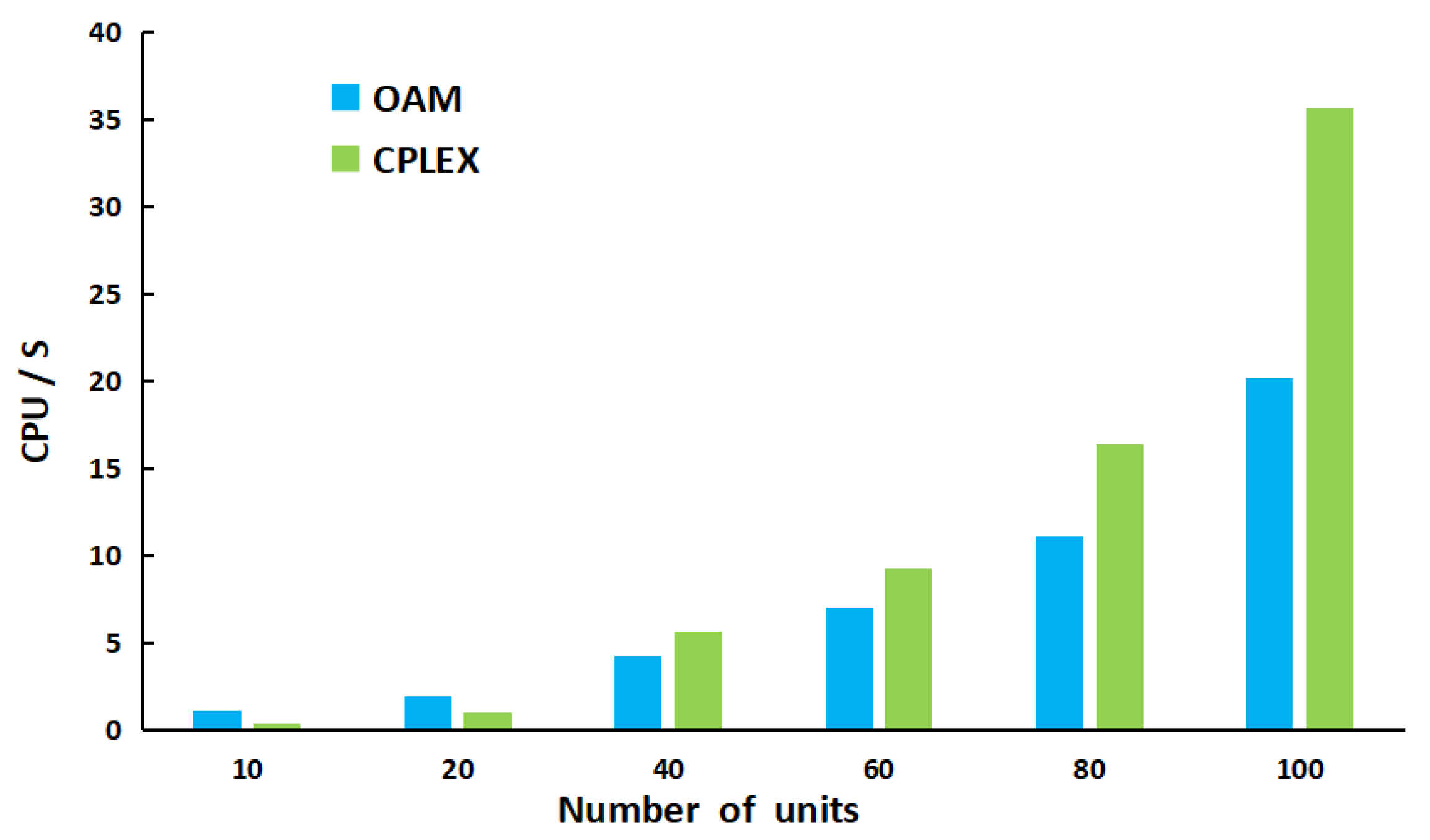
	10	20	40	60	80	100
OAM	772,385	1,589,870	3,186,766	5,011,717	6,674,541	8,351,644
CPLEX	788,539	1,596,907	3,189,870	5,025,949	6,709,200	8,393,972

. Figure 1 shows the comparison of the calculation time of the two methods. It can be seen that as the number of units increases, the advantages of the OAM algorithm can be reflected. Therefore, OAM is very useful for large-scale practical engineering application problems. From Table 3, the OAM has a lower total operation cost than CPLEX. This is because the OA($\Omega$) obtained by linearization at the optimal solution of the continuous relaxation problem of MINLP (14) can better approximate. In addition, OAM obtains the lower and upper bound of the optimal value of MINLP (14) by solving OA($\Omega$) and $\mathrm{NLP}\left(u^{k+1}\right)$, respectively, which approaches the optimal value of MINLP (14) by continuously reducing the upper bound and increasing the lower bound.

In order to further illustrate the effectiveness of OAM to solve the problem and the practicality of the model proposed in this paper,

Table 4. Comparison total operation cost of three models.

	Consider the Wind Power Curtailment and Pollutant Emissions	Consider the Wind Power Curtailment	Consider the Pollutant Emission
10	772,385	789,549	793,467
20	1,589,870	1,596,910	1,650,468
40	3,186,766	3,189,860	3,245,780
60	5,011,717	5,015,879	5,134,660
80	6,674,541	6,725,780	6,878,905
100	8,351,644	8,493,672	8,656,076

shows the total system cost comparison results of the three models, which consider both wind power curtailment and pollutant emissions and only consider the total cost of wind power curtailment, as well as only consider the total cost of pollutant emissions. According to Table 4, we can find that the cost of considering both wind curtailment and pollutant emission is the lowest, and it has better economic benefits in practical engineering applications.

In order to explain the results in more detail,

Table 5. The output and pollutant emission for the 10 thermal units.

Hour	Unit										Pollutant Emissions
	1	2	3	4	5	6	7	8	9	10
1	228	228	25	29	40	20	25	10	10	10	4352
2	189	173	57	55	66	36	25	21	21	20	3326
3	187	171	90	81	92	52	25	32	23	18	3491
4	195	180	96	107	118	68	25	41	29	24	3879
5	198	183	97	121	130	80	26	43	32	27	4104
6	218	202	108	130	130	80	39	54	43	38	4615
7	223	208	112	126	130	80	43	44	44	42	4712
8	249	234	127	104	123	64	60	44	44	44	5141
9	299	283	130	104	104	64	68	44	44	44	6536
10	338	323	130	117	130	77	68	44	44	44	8028
11	364	358	130	104	124	64	68	42	42	42	9006
12	389	374	162	130	130	80	85	31	31	31	10,482
13	363	348	162	130	130	80	84	20	20	20	9499
14	347	332	162	130	130	80	67	0	0	0	7985
15	306	291	159	130	130	80	50	0	0	0	6547
16	271	256	140	130	130	80	0	0	0	0	5096
17	271	255	130	111	130	69	0	0	0	0	4821
18	309	294	130	106	130	64	0	0	0	0	5872
19	364	364	130	104	104	64	0	0	0	0	7939
20	362	346	162	130	130	80	50	20	20	20	9348
21	283	361	162	130	130	80	61	0	0	0	7449
22	192	364	130	104	104	64	44	0	0	0	5745
23	0	339	162	130	130	80	0	0	0	0	4947
24	0	254	139	130	130	80	0	0	0	0	3389

gives the output and pollutant emission of each unit for 10 thermal units over the scheduling period of 24 h. We set the weight factors $w_t=w_e=1$ and the pollutant emission penalty factor ${\pi }_i=1\$\left(\mathrm{Ton}\right)$$(i=1,\cdots ,N)$. It can be seen from Table 5 that the total amount of pollutant emission for 10 thermal units is 131,261$\left(\mathrm{Ton}\right)$ and the pollutant emission cost is 131,261$. Therefore, the pollutant emission costs cannot be ignored.

The following

Table 6. System operating cost, pollutant emission, wind power utilization.

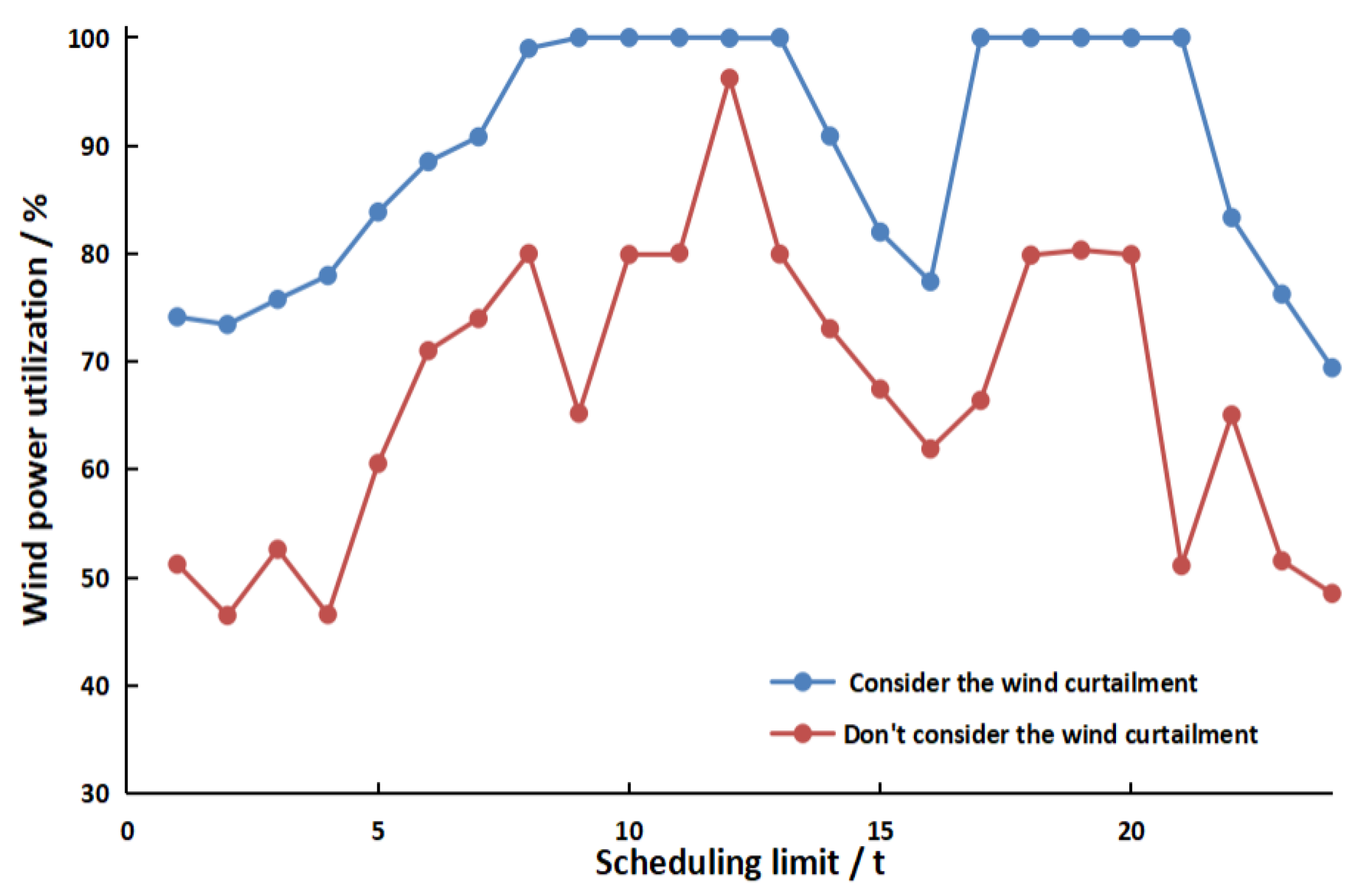
Mode	Total Operating Cost/$	Pollutant Emission/t	Wind Power Utilization/%
Consider wind curtailment	772,385	131,261	82.43
Do not consider wind curtailment	838,409	148,976	64.45

shows the comparison results of the total operating cost and wind power utilization rate as well as pollutant emissions in two cases, which is whether the wind curtailment is considered. It can be seen from Table 6 that the wind power utilization rate increases and the pollutant emissions and total system cost are reduced when the wind curtailment is considered. Therefore, the UC problem with wind curtailment and pollutant emission has better economic efficiency and high practical value.

In order to show more clearly the necessity of considering wind curtailment in the model in this paper, Figure 2 shows how the wind power utilization rate in 24 periods is compared, i.e., including and excluding the wind curtailment. Obviously, the utilization rate of wind power after considering wind curtailment is higher than without consideration.

5. Conclusions

This paper presents an MIQP model of the UC problem with wind power curtailment and pollutant emissions by some linearization techniques, and then OAM is used to solve the equivalent form of MIQP. The results of six systems with thermal units from 10 to 100 and one wind unit over a scheduling period of 24 h show that OAM can solve the equivalent form of MIQP more quickly and effectively, and it has better numerical performance than CPLEX. OAM is suitable for solving the large-scale UC problem. In addition, the numerical simulation results corresponding to a situation where the wind curtailment is considered show that the model proposed in this paper is reasonable.

References

- Li, X.; Zhai, Q.; Zhou, J.; Guan, X. A Variable Reduction Method for Large-Scale Unit Commitment. IEEE Trans. Power Syst. 2020, 35, 261–272. [Google Scholar] [CrossRef]
- Wang, C.; Sun, H.; Liang, J.; Niu, Y. The study of unit commitment considering wind forecasting power. In Proceedings of the International Conference on Power System Technology, Chengdu, China, 20–22 October 2014; pp. 2614–2617. [Google Scholar]
- Sundar, K.; Nagarajan, H.; Roald, L.; Misra, S.; Bent, R.; Bienstock, D. Chance-Constrained Unit Commitment with N-1 Security and Wind Uncertainty. IEEE Control Netw. Syst. 2019, 6, 1062–1074. [Google Scholar] [CrossRef]
- Wu, Z.; Zeng, P.; Zhang, X.; Zhou, Q. A Solution to the Chance-Constrained Two-Stage Stochastic Program for Unit Commitment with Wind Energy Integration. IEEE Trans. Power Syst. 2016, 31, 4185–4196. [Google Scholar] [CrossRef]
- Wang, C.; Liu, F.; Wei, W.; Mei, S.; Qiu, F.; Wang, J. Robust unit commitment considering strategic wind generation curtailment. In Proceedings of the IEEE Power and Energy Society General Meeting (PESGM), Boston, MA, USA, 17–21 July 2016; pp. 1–5. [Google Scholar]
- Yang, B.; Cao, X.; Cai, Z.; Yang, T.; Chen, D.; Gao, X.; Zhang, J. Unit Commitment Comprehensive Optimal Model Considering the Cost of Wind Power Curtailment and Deep Peak Regulation of Thermal Unit. IEEE Access 2020, 8, 71318–71325. [Google Scholar] [CrossRef]
- Wu, X.; Zhang, B.; Wang, K.; Li, J.; Duan, Y. A Quantum-inspired Binary PSO algorithm for unit commitment with wind farms considering emission reduction. In Proceedings of the IEEE PES Innovative Smart Grid Technologies, Tianjin, China, 21–24 May 2012; pp. 1–6. [Google Scholar]
- Ding, T.; Zeng, Z.; Qu, M.; Catalão, J.P.S.; Shahidehpour, M. Two-Stage Chance-Constrained Stochastic Thermal Unit Commitment for Optimal Provision of Virtual Inertia in Wind-Storage Systems. IEEE Trans. Power Syst. 2021, 36, 3520–3530. [Google Scholar] [CrossRef]
- Lei, S.; Hou, Y.; Wang, X.; Liu, K. Unit Commitment Incorporating Spatial Distribution Control of Air Pollutant Dispersion. IEEE Trans. Ind. Inf. 2017, 13, 995–1005. [Google Scholar] [CrossRef]
- Zhang, Z.; Chen, Y.; Liu, X.; Wang, W. Two-Stage Robust Security-Constrained Unit Commitment Model Considering Time Autocorrelation of Wind/Load Prediction Error and Outage Contingency Probability of Units. IEEE Access 2019, 7, 25398–25408. [Google Scholar] [CrossRef]
- Wang, Y.; Lou, S.; Wu, Y.; Lv, M. Robust Unit Commitment and Dispatch Considering with Atmospheric Pollutant Concentration Constraints. In Proceedings of the IEEE Power and Energy Society General Meeting (PESGM), Portland, OR, USA, 5–10 August 2018; pp. 1–5. [Google Scholar]
- Bian, Q.; Xin, H.; Wang, Z.; Gan, D.; Wong, K.P. Distributionally Robust Solution to the Reserve Scheduling Problem with Partial Information of Wind Power. IEEE Trans. Power Syst. 2015, 30, 995–1005. [Google Scholar] [CrossRef]
- Xiong, P.; Jirutitijaroen, P.; Singh, C. A Distributionally Robust Optimization Model for Unit Commitment Considering Uncertain Wind Power Generation. IEEE Trans. Power Syst. 2017, 32, 39–49. [Google Scholar] [CrossRef]
- Liu, R.; Hou, Y.; Li, Y.; Lei, S.; Wei, W.; Wang, X. Sample Robust Scheduling of Electricity-Gas Systems Under Wind Power Uncertainty. IEEE Trans. Power Syst. 2021, 1, 5889–5900. [Google Scholar] [CrossRef]
- Tien, M.; Andrea, L. A multicut outer-approximation approach for competitive facility location under random utilities. Eur. J. Oper. Res. 2020, 284, 874–881. [Google Scholar]
- Carrion, W.; Arroyo, J.M. A computationally efficient mixed-integer linear formulation for the thermal unit commitment problem. IEEE Trans. Power Syst. 2006, 21, 1371–1378. [Google Scholar] [CrossRef]
- Morales-España, G.; Latorre, J.M.; Ramos, A. Tight and Compact MILP Formulation for the Thermal Unit Commitment Problem. IEEE Trans. Power Syst. 2013, 28, 4897–4908. [Google Scholar] [CrossRef]
- Ongsakul, W.; Petcharaks, N. Unit commitment by enhanced adaptive Lagrangian relaxation. IEEE Trans. Power Syst. 2004, 1, 620–628. [Google Scholar] [CrossRef]
- Pereira, F.B.; Paucar, V.L.; Saraiva, F.S. Power System Unit Commitment Incorporating Wind Energy and Battery Energy Storage. In Proceedings of the IEEE XXV International Conference on Electronics, Electrical Engineering and Computing (INTERCON), Lima, Peru, 8–10 August 2018; pp. 1–4. [Google Scholar]
- Zhenhua, C.; Lixiong, L. Calculation of the critical value of abandoned wind considering the cost of wind curtailment and the cost of deep peak regulation. J. Hunan Univ. Nat. Sci. Ed. 2021, 30, 65–69. (In Chinese) [Google Scholar]
- IBM ILOG CPLEX Optimization Studio [EB/OL]. Available online: https://www.ibm.com/prodUCts/ilog-cplex-optimization-studio (accessed on 5 January 2020).