Mixed Convection Stagnation Point Flow of a Hybrid Nanofluid Past a Permeable Flat Plate with Radiation Effect

Abstract

This article focuses on the stagnation point flow of hybrid nanofluid towards a flat plate. The cases when the buoyancy forces and the flow are in the opposite direction and the same direction are discussed. The effect of radiation and suction is also taken into account. The similarity transformations are used to convert the partial differential equations into nonlinear ordinary differential equations. These equations are computed numerically via the bvp4c function in MATLAB software. A comparison with the previously published articles is carried out, where an outstanding agreement is observed. The dual solutions exist in the case of opposing flow $(\lambda <0)$ and the suction parameter $S>0.6688$. Meanwhile, only unique solutions exist in the case of assisting flow $(\lambda >0)$. The existence of dual solutions leads to stability analysis. From the analysis, the first solution is confirmed as a stable solution. Furthermore, the heat transmission rate increases, while the skin friction coefficient decreases as the radiation rate increases. An increase in the radiation rate from 0 (no radiation) to $1.0$ increases the heat transmission rate by $5.01\%$ for water, $4.96\%$ for nanofluid, and $4.80\%$ for hybrid nanofluid. Finally, it is worth mentioning that the present study yields new and original results. This study has also not been done by other researchers, indicating its novelty.

1. Introduction

Over the last few decades, the topic of nanofluid has attracted a vast number of researchers due to its contribution to industries. Note that the study of nanofluid flow was proposed by Choi and Eastman [1]. Nanofluid is a homogenous mixture of nanoparticles (i.e., metals, metal oxides, and carbon materials) and regular fluids (i.e., water, ethylene glycol, and oil). In contrast to regular fluids, nanofluids possess one-phase heat transfer coefficients and have larger thermal conductivity. Through the years, many investigations for development purposes have been conducted for enhancing heat transfer performance in certain flow problems. A new kind of fluid, namely hybrid nanofluid, is introduced by suspending two different nanoparticles in the regular fluid. By combining these nanoparticles, their chemical and physical properties will simultaneously combine and lead those properties in a homogeneous state [2,3]. The reviews on the preparation, thermophysical properties, and applications of hybrid nanofluid have been studied by several authors [4,5,6,7,8,9,10,11,12,13]. Recently, some published works have been reported for estimating the properties of both nanofluids and hybrid nanofluids. Esfe et al. [14] studied the thermal properties of Mg/O water nanofluid using artificial neural networks (ANNs). Later on, Fuxi et al. [15] investigated the thermal characteristics of water-EG/MWCNT-Al${}_2$O${}_3$ hybrid nanofluid using a feed-forward neural network. The effect of nanoparticle volume fraction and temperature on dynamics viscosity of Al${}_2$O${}_3$-MWCNT (40:60)-Oil SAE50 hybrid nanofluid is examined by Qing et al. [16]. Esfe and Toghraie [17] applied an optimal feed-forward artificial neural network model and new empirical correlation to predict the viscosity of Al${}_2$O${}_3$-engine oil nanofluid. It is found that ANN estimated laboratory data more accurately than correlation output and ANN output.

Hybrid nanofluids have multitudinous applications in thermal energy transport, especially in manufacturing, naval structures, microfluidics, defense, transportation, acoustics, and biomedical [5,6,8]. Motivated by these important applications, numerous studies have been done to study the hybrid nanofluid in the boundary layer flow. For example, Devi and Devi [18] performed the hybrid nanofluid flow and heat transfer analysis over a stretching surface. They observed that the hybrid nanofluid had a higher heat transfer rate compared to nanofluid. Apart from that, Yousefi et al. [19] carried out an analytical study of the stagnation point flow near a cylindrical surface in a hybrid nanofluid. Their study showed that the thermal characteristics of the regular fluid are smaller compared to hybrid nanofluid and nanofluid with single nanoparticles. Moreover, Muhammad et al. [20] considered the stagnation point flow past a stretching sheet using cupric oxide (CuO) and carbon nanotubes (CNTs) with gasoline oil. Furthermore, continuous studies on hybrid nanofluid have been performed by many authors using various surfaces and physical situations [21,22,23,24,25,26].

The fluid motion near the stagnation region of a solid body is known as a stagnation point flow. The stagnation point flow can be defined as a point located at the object surface in the flow with zero local fluid velocity. In the stagnation region, the object leads the fluid to rest. When the fluid velocity is absent, the static pressure is at its highest magnitude at the stagnation point. The analysis of the stagnation point received much attention from researchers due to their important applications in some fields including nuclear reactor cooling systems, electronics cooling systems, aerospace, and so forth [27]. The stagnation point flow past a stationary semi-infinite plate was first discussed by Hiemenz [28], who applied the similarity variables to reduce the Navier–Stokes equations to nonlinear ordinary differential equations. Furthermore, consideration of mixed convection in stagnation point flow is one of the interesting topics on which to conduct research. In the presence of mixed convection, the buoyancy forces are caused by the temperature difference between the free stream and the surface enhancement. This leads to altering the flow as well as the thermal field. In this situation, the symmetrical behavior of the flow and thermal fields no longer exists concerning the stagnation line [29]. Other than that, this situation can also increase or decrease both local shear stress and heat transfer compared to forced convection flow.

Mixed convection flow near a stagnation point finds its applications in heat exchangers, electronic devices, solar and nuclear reactors, and atmospheric boundary layer flows. Comprehensive references on this topic can be found in the reported articles. Moreover, Tamim et al. [30] studied the MHD mixed convection stagnation point flow near a permeable surface in a nanofluid. In their study, the flow is subjected to prescribed surface temperature and external flow. Later on, Dinarvand et al. [31] examined the stagnation point flow of a nanofluid towards a vertical permeable stretching or shrinking plate. In addition, Rostami et al. [32] obtained two solutions for the mixed convective stagnation point flow of an aqueous silica-alumina hybrid nanofluid using the bvp4c solver. They found that the thermophysical characteristics of nanofluid and regular fluid can be enhanced by suspending two different nanoparticles. Finally, the study of combined free and forced convection flow in a stagnation region past a stretchable surface is considered by Seth et al. [33]. Thereafter, Zainal et al. [34] attempted to study the impact of convective boundary conditions and magnetic field on the flow towards a vertical flat surface in a hybrid nanofluid. The latest published work on mixed convection stagnation point flow is discussed by Ali et al. [35] under the influence of radiation and a magnetic field near a vertical stretching surface.

The boundary layer analysis with radiative heat flux is highly significant in the area of processes and space technology that requires high-temperature [36]. Radiation effects have numerous applications, for instance, in astrophysical flows, electricity generation, and solar power technologies. However, the addition of radiation in the thermal energy equation drives a highly nonlinear partial differential equation. Several works have been conducted to study the radiation effect in the boundary layer flow. For example, Turkyilmazoglu and Pop [37] performed an analytical study of a nanofluid flow adjacent to a vertical surface with the influence of radiation. The flow towards a permeable shrinking surface in a Casson fluid with inconstant surface temperature and radiation was examined by Bhattacharyya et al. [38]. Moreover, Soomro et al. [39] analyzed the influence of heat generation/absorption and radiation on the stagnation point flow near a stretching plate in a nanofluid. In addition, Jha and Samaila [40] numerically studied the thermal boundary layer flow on a flat surface with the convective boundary condition and thermal radiation effect. Furthermore, Anuar et al. [41] performed the unsteady micropolar hybrid nanofluid flow past a deformable sheet in the stagnation region. They noticed that the addition of radiation increased the heat transfer rate. Very recently, Jamaludin et al. [42] considered the mixed convection stagnation point flow in a cross fluid towards a permeable shrinking surface with radiation and suction effects.

Motivated by the above-mentioned articles, the novelty of the current work is to explore the existence of two solutions and the effect of radiation in mixed convection stagnation point flow near a permeable flat plate in Al${}_2$O${}_3$-Cu hybrid nanofluid. This problem follows the nanofluid correlations proposed by Devi and Devi [18]. It is worth mentioning that this problem has not been analyzed in any of the referenced state-of-the-art reviews before. To simplify the system of equations, the partial differential equations are converted into a non-dimensional form. The solutions for these equations are executed using the bvp4c package in the MATLAB program. Moreover, the use of this numerical method is inspired by the work of Rostami et al. [32], where several examinations are performed to figure out the accuracy of the current model. The current results are compared with several published articles for validation purposes. The physical reliability of the dual solutions gained is determined using stability analysis.

2. Description and Formulation of the Model

We considered a steady stagnation point flow of a hybrid nanofluid over a vertical flat plate with the effect of suction and radiation as shown in Figure 1. The x-axis is taken along the flat plate, while the y-axis is perpendicular to the surface of the plate. It is assumed that the ambient velocity of the flow is $u_e\left(x\right)=cx$, where c is a constant with $c>0$. The surface temperature is $T_s\left(x\right)=T_{\infty }+T^{*}(x/L)$, where $T_{\infty }$ is the ambient temperature, $T^{*}$ is the characteristic temperature and L is the characteristic length of the surface. The opposing flow ($T^{*}<0$) occurs when the upper part of the surface is cooled while the lower part of the surface is heated. In contrast, the assisting flow ($T^{*}>0$) occurs when the upper part of the surface is heated while the lower part of the surface is cooled. In this case, with the presence of buoyancy forces, the flow near the heated surface tends to move upward while the flow near the cooled surface tends to move downward. Hence, this behavior acts to assist the flow field [43].

Under the aforementioned assumptions, the governing equations are [30]:

$$u_x+v_y=0,$$

(1)

$$u{u}_x+v{u}_y=u_e{\left(u_e\right)}_x+\frac{{\mu }_{hnf}}{{\rho }_{hnf}}{u}_{yy}+{\beta }_{hnf}g(T-T_{\infty }),$$

(2)

$$u{T}_x+v{T}_y=\frac{k_{hnf}}{{\left(\rho C_p\right)}_{hnf}}{T}_{yy}-\frac{{\left(q_r\right)}_y}{{\left(\rho C_p\right)}_{hnf}},$$

(3)

subject to [32]

$$u=0,v=v_0,T=T_s\left(x\right)\mathrm{at}y=0,$$

$$u\to u_e\left(x\right),T\to T_{\infty }\mathrm{as}y\to \infty ,$$

(4)

where $(u,v)$ are the velocity fields of x and y directions. Respectively, g is the gravitational acceleration and T is the fluid temperature. The uniform mass flux is denoted by $v_0$, where $v_0>0$ for injection and $v_0<0$ for suction.

The radiative heat flux under Rosseland approximation is $q_r$, which is given by [44]:

$$q_r=-\frac{4{\sigma }^{*}{\left(T^4\right)}_y}{3k^{*}}.$$

(5)

In the above equation, ${\sigma }^{*}$ is the Stefan–Boltzman constant, while $k^{*}$ is the mean absorption coefficient. It is assumed that the temperature differences within the hybrid nanofluid are $T^4$, which can be expressed as a linear function of temperature. Expanding the term $T^4$ in a Taylor series about $T_{\infty }$ and neglecting higher-order terms, $T^4$ can be written as [44]:

$$T^4\cong 4T_{\infty }^{3}T-3T_{\infty }^4.$$

(6)

Thus, Equation (3) can be expressed as follows:

$$u{T}_x+v{T}_y=\frac{1}{{\left(\rho C_p\right)}_{hnf}}\left(k_{hnf}+\frac{16{\sigma }^{*}{T}_{\infty }^3}{3k^{*}}\right)T_{yy}.$$

(7)

The applied models for physical characteristics of hybrid nanofluid and nanofluid are given in

Table 1. Applied models for physical characteristics of hybrid nanofluid and nanofluid (see Devi and Devi [18]).

	Hybrid Nanofluid
Dynamic viscosity, $\mu$	${\mu }_{hnf}={\mu }_f{(1-{\phi }_1)}^{-2.5}{(1-{\phi }_2)}^{-2.5}$
Buoyancy coefficient, $\beta$	${\left(\rho \beta \right)}_{hnf}=\left[(1-{\phi }_1){\left(\rho \beta \right)}_f+{\phi }_1{\left(\rho \beta \right)}_{s1}\right](1-{\phi }_2)+{\phi }_2{\left(\rho \beta \right)}_{s2}$
Density, $\rho$	${\rho }_{hnf}=\left[(1-{\phi }_1){\rho }_f+{\phi }_1{\rho }_{s1}\right](1-{\phi }_2)+{\phi }_2{\rho }_{s2}$
Heat capacity, $\rho C_p$	${\left(\rho C_p\right)}_{hnf}=\left[(1-{\phi }_1){\left(\rho C_p\right)}_f+{\phi }_1{\left(\rho C_p\right)}_{s1}\right](1-{\phi }_2)$
	$+{\phi }_2{\left(\rho C_p\right)}_{s2}$
Thermal conductivity, k	$k_{hnf}=\frac{k_{s2}+2k_{bf}-2{\phi }_2(k_{bf}-k_{s2})}{k_{s2}+2k_{bf}+{\phi }_2(k_{bf}-k_{s2})}{k}_{bf}$ where
	$k_{bf}=\frac{k_{s1}+2k_f-2{\phi }_1(k_f-k_{s1})}{k_{s1}+2k_f+{\phi }_1(k_f-k_{s1})}{k}_f$
	Nanofluid
Dynamic viscosity, $\mu$	${\mu }_{nf}={\mu }_f{(1-\phi )}^{-2.5}$
Buoyancy coefficient, $\beta$	${\left(\rho \beta \right)}_{nf}={\left(\rho \beta \right)}_f(1-\phi )+\phi {\left(\rho \beta \right)}_s$
Density, $\rho$	${\rho }_{nf}={\rho }_f(1-\phi )+\phi {\rho }_s$
Heat capacity, $\rho C_p$	${\left(\rho C_p\right)}_{nf}={\left(\rho C_p\right)}_f(1-\phi )+\phi {\left(\rho C_p\right)}_s$
Thermal conductivity, k	$k_{nf}=\frac{k_s+2k_f-2\phi (k_f-k_s)}{k_s+2k_f+\phi (k_f-k_s)}{k}_f$

. In the table, the subscript $hnf$, f, $nf$ and s refers to hybrid nanofluid, fluid, nanofluid and solid nanoparticle, where $s1$ and $s2$ are the first and second nanoparticles, respectively. The nanoparticle volume fraction parameter is denoted as $\phi$, where ${\phi }_1$ is the nanoparticle volume fraction for alumina, and ${\phi }_2$ is the nanoparticle volume fraction for copper. The thermophysical characteristics of copper (Cu), alumina (Al${}_2$O${}_3$), and the regular fluid (water) are tabulated in

Table 2. Physical properties of nanoparticles and the regular fluid [45].

Properties	${\mathit{C}}_{\mathit{p}}$ (J/kgK)	$\mathit{\rho }$ (kg/m${}^3$)	k (W/mK)
Cu	8933	400	385
Al${}_2$O${}_3$	3970	40	765
Water	997.1	0.6071	4180

.

The following similarity variables are introduced to convert our model into dimensionless form [30].

$$u=cx{f}^{\prime }\left(\xi \right),v=-\sqrt{c{\nu }_f}f\left(\xi \right),\xi =y\sqrt{\frac{c}{{\nu }_f}},\theta \left(\xi \right)=\frac{T-T_{\infty }}{T_s-T_{\infty }}.$$

(8)

The uniform mass flux for the permeable surface is given by [32]

$$v_0=-\sqrt{c{\nu }_f}S,$$

(9)

where S is the mass flux variable with $S<0$ for injection and $S>0$ for suction.

Upon substituting Equation (8), Equation (1) is satisfied and Equations (2) and (7) become:

$$\frac{C_1}{C_2}{f}^{‴}+f{f}^{″}-{\left(f^{\prime }\right)}^2+C_3\lambda \theta +1=0,$$

(10)

$$\frac{1}{D_1\mathrm{P}\mathrm{r}}\left(D_2+\frac{4Rd}{3}\right){\theta }^{″}+f{\theta }^{\prime }-f^{\prime }\theta =0,$$

(11)

where $C_1={\mu }_{hnf}/{\mu }_f$, $C_2={\rho }_{hnf}/{\rho }_f$, $C_3={\beta }_{hnf}/{\beta }_f$, $D_1={\left(\rho C_p\right)}_{hnf}/{\left(\rho C_p\right)}_f$ and $D_2=k_{hnf}/k_f$. The transformed boundary condition can be written as:

$$f\left(0\right)=S,f^{\prime }\left(0\right)=0,\theta \left(0\right)=1,$$

$$f^{\prime }(\infty )\to 1,\theta (\infty )\to 0,$$

(12)

where prime is the differentiation with respect to $\xi$, Pr is the usual Prandtl number, $Rd$ is the radiation parameter, and $\lambda$ is the mixed convection parameter. The mentioned variables can be expressed as follows:

$$\mathrm{P}\mathrm{r}=\frac{{\left(\rho C_p\right)}_f}{k_f},Rd=\frac{4{\sigma }^{*}}{k^{*}}\frac{T_{\infty }^3}{k_f},\lambda =\frac{G{r}_x}{R{e}_x^2}.$$

(13)

Here, $R{e}_x=u_e\left(x\right)x/{\nu }_f$ is the local Reynolds number and $G{r}_x=g{\beta }_f(T_s-T_{\infty })x^3/{\nu }_f^2$ is the local Grashof number. It is worth mentioning that, when ${\phi }_1={\phi }_2=0$ (regular fluid), $Rd=0$ (radiation effects are negligible) and $S=0$ (impermeable plate), Equations (10)–(12) reduced to those studied by Ramachandran [29].

The physical quantities of the skin friction coefficient, $C_f$ and the local Nusselt number, $N{u}_x$, are defined as follows [32]:

$$C_f=\frac{{\tau }_s}{{\rho }_f{u}_e^2}\mathrm{and}N{u}_x=\frac{x{q}_s}{k_f\left(T_s-T_{\infty }\right)},$$

(14)

where the shear stress of the plate, ${\tau }_s$, and the heat flux of the plate, $q_s$, are given by [39]:

$${\tau }_s={\mu }_{hnf}\left(\frac{\partial u}{\partial y}\right){|}_{y=0},q_s=-k_{hnf}\left(\frac{\partial T}{\partial y}\right){{|}_{y=0}+\left(q_r\right)|}_{y=0}.$$

(15)

Using Equations (8) and (15), Equation (14) then becomes:

$$R{e}_x^{1/2}{C}_f=C_1{f}^{″}\left(0\right)andR{e}_x^{-1/2}N{u}_x=-\left(D_2+\frac{4}{3}Rd\right){\theta }^{\prime }\left(0\right).$$

(16)

3. Stability Analysis

Stability analysis is an analysis for identifying the stability of the solutions obtained. The similarity solutions emerge from Equations (10) and (11) subject to the boundary conditions (12). Note that several studies related to stability analysis have been done by other researchers [32,46,47,48,49]. The procedures used in this analysis are referred to from the work of Merkin [50], Weidman et al. [51], and Harris et al. [52]. Following these three papers, the unsteady problem is initially considered as follows:

$$u_t+u{u}_x+v{u}_y=u_e{\left(u_e\right)}_x+\frac{{\mu }_{hnf}}{{\rho }_{hnf}}{u}_{yy}+{\beta }_{hnf}g(T-T_{\infty }),$$

(17)

$$T_t+u{T}_x+v{T}_y=\frac{k_{hnf}}{{\left(\rho C_p\right)}_{hnf}}{T}_{yy}-\frac{{\left(q_r\right)}_y}{{\left(\rho C_p\right)}_{hnf}}.$$

(18)

Afterward, the dimensionless time variable, $\tau =ct$, is introduced. Thus, the following new similarity variables are obtained:

$$u=cx{f}^{\prime }(\xi ,\tau ),v=-\sqrt{c{\nu }_f}f(\xi ,\tau ),\xi =y\sqrt{\frac{c}{{\nu }_f}},\theta (\xi ,\tau )=\frac{T-T_{\infty }}{T_s-T_{\infty }},\tau =ct.$$

(19)

Considering terms from Equations (13) and (19), Equations (17) and (18) are converted into the following:

$$\frac{C_1}{C_2}\frac{{\partial }^{3}f}{\partial {\xi }^3}+f\frac{{\partial }^{2}f}{\partial {\xi }^2}-{\left(\frac{\partial f}{\partial \xi }\right)}^2+C_3\lambda \theta +1-\frac{{\partial }^{2}f}{\partial \xi \partial \tau }=0,$$

(20)

$$\frac{1}{\mathrm{P}\mathrm{r}{D}_1}\left(D_2+\frac{4}{3}Rd\right)\frac{{\partial }^2\theta }{\partial {\xi }^2}+f\frac{\partial \theta }{\partial \xi }-\frac{\partial f}{\partial \xi }\theta -\frac{\partial \theta }{\partial \tau }=0,$$

(21)

subject to the boundary conditions

$$f(0,\tau )=S,\frac{\partial f}{\partial \xi }(0,\tau )=0,\theta (0,\tau )=1,$$

$$\frac{\partial f}{\partial \xi }(\infty ,\tau )\to 1,\theta (\infty ,\tau )\to 0.$$

(22)

According to Weidman et al. [51], the similarity solutions are determined by substituting Equation (23) into Equations (20)–(22) with $f=f_0\left(\xi \right)$ and $\theta ={\theta }_0\left(\xi \right)$.

$$f(\xi ,\tau )=f_0\left(\xi \right)+e^{-\zeta \tau }F(\xi ,\tau ),\theta (\xi ,\tau )={\theta }_0\left(\xi \right)+e^{-\zeta \tau }G(\xi ,\tau ).$$

(23)

From the above equation, $\zeta$ is the eigenvalue and $F(\xi ,\tau )$ and $G(\xi ,\tau )$ are assumed to be small, relative to $f_0\left(\xi \right)$ and ${\theta }_0\left(\xi \right)$, respectively.

The linearized eigenvalue equations associated with the current problem are:

$$\frac{C_1}{C_2}{F}_0^{‴}+f_0{F}_0^{″}+F_0{f}_0^{″}-2f_0^{\prime }{F}_0^{\prime }+C_3\lambda G_0+\zeta F_0^{\prime }=0,$$

(24)

$$\frac{1}{\mathrm{P}\mathrm{r}{D}_1}\left(D_2+\frac{4}{3}Rd\right)G_0^{″}+f_0{G}_0^{\prime }+F_0{\theta }_0^{\prime }-f_0^{\prime }{G}_0-F_0^{\prime }{\theta }_0+\zeta G_0=0,$$

(25)

together with the boundary conditions

$$F_0\left(0\right)=0,F_0^{\prime }\left(0\right)=0,G_0\left(0\right)=0,$$

$$F_0^{\prime }(\infty )\to 0,G_0(\infty )\to 0.$$

(26)

As discussed by Weidman et al. [51], $\tau$ is assumed to be zero indicating an initial decline or rise of the solution (23). Besides, the terms $F(\xi ,\tau )$ and $G(\xi ,\tau )$ can be expressed as $F_0\left(\xi \right)$ and $G_0\left(\xi \right)$, respectively. Harris et al. [52] stressed that it is necessary to relax one of the far field boundary conditions (26) whether on $F_0^{\prime }\left(\xi \right)$ or $G_0\left(\xi \right)$. In this work, we relaxed the condition $F_0^{\prime }\left(\xi \right)\to 0$ as $\xi \to \infty$ and replaced it with a new condition $F_0^{″}\left(0\right)=1$.

4. Method of Solutions

Computation of results for Equations (10)–(12) is performed by using the bvp4c solver in MATLAB software. The solver is programmed with a collocation method with fourth-order accuracy (see Shampine et al. [53]). It is one of the effective techniques for solving boundary value problems (BVPs) for ordinary differential equations. The solver requires three kinds of information such as the equation to be solved, its related boundary conditions, and an initial guess for the solution. Mathematically, the bvp4c solver uses the finite difference method, where the output is obtained using an initial guess supplied at the starting mesh points. It is necessary to change the step size to obtain proper precisions. Since BVPs can have more than one solution, the program requires users to supply a guess for the solution desired.

Before importing the model into the solver, Equations (10)–(12) must be converted into a system of first-order as follows [53]:

$$y\left(1\right)=f\left(\xi \right),y\left(2\right)=f^{\prime }\left(\xi \right),y\left(3\right)=f^{″}\left(\xi \right),y\left(4\right)=\theta \left(\xi \right),y\left(5\right)={\theta }^{\prime }\left(\xi \right),$$

(27)

$$f^{‴}=-\frac{C_2}{C_1}\left[y\left(1\right)y\left(3\right)-y\left(2\right)y\left(2\right)+C_3\lambda y\left(4\right)+1\right],$$

(28)

$${\theta }^{″}=-\frac{1}{\left(D_2+\frac{4}{3}Rd\right)}\mathrm{P}\mathrm{r}{D}_1\left[y\left(1\right)y\left(5\right)-y\left(2\right)y\left(4\right)\right],$$

(29)

and

$$ya\left(1\right)=S,ya\left(2\right)=0,ya\left(4\right)=1,$$

$$yb\left(2\right)\to 1,yb\left(4\right)\to 0.$$

(30)

Here, a is the condition at the surface $(\xi =0)$ while b is the condition at the free stream $(\xi =\infty )$.

Next, the appropriate boundary layer thickness, initial guesses and inputs of the physical parameters (i.e., $Rd$, S, $\lambda$, $\mathrm{P}\mathrm{r}$, ${\phi }_1$ and ${\phi }_2$) must be set to compute the desired solution. The numerical solution can be accepted when the boundary conditions ($f^{\prime }\left(\xi \right)\to 1$, $\theta \left(\xi \right)\to 0$ as $\xi \to \infty$) are contented and there is an error or warning produced during the execution. The boundary conditions at $\xi \to \infty$ are substituted by $\xi ={\xi }_{\infty }$. In this work, the appropriate value of $\xi$ is chosen as ${\xi }_{\infty }=10$, where ${\xi }_{\infty }$ is situated outside the boundary layer thickness. The procedures are repeated to ensure the converged result secures a tolerance limit of ${10}^{-6}$ [48]. The obtained results are then presented in tables and are plotted graphically.

Since we obtained two solutions, the stability analysis is performed to validate the stability of the solutions. In importing this analysis, the same procedures as above are applied using Equations (24)–(26) [53].

$$y\left(1\right)=F_0\left(\xi \right),y\left(2\right)=F_0^{\prime }\left(\xi \right),y\left(3\right)=F_0^{″}\left(\xi \right),y\left(4\right)=G_0\left(\xi \right),y\left(5\right)=G_0^{\prime }\left(\xi \right),$$

(31)

$$s\left(1\right)=f_0\left(\xi \right),s\left(2\right)=f_0^{\prime }\left(\xi \right),s\left(3\right)=f_0^{″}\left(\xi \right),s\left(4\right)={\theta }_0\left(\xi \right),s\left(5\right)={\theta }_0^{\prime }\left(\xi \right),$$

(32)

$$F_0^{‴}=-\frac{C_2}{C_1}\left[s\left(1\right)y\left(3\right)+y\left(1\right)s\left(3\right)-2s\left(2\right)y\left(2\right)+C_3\lambda y\left(4\right)+\zeta y\left(F_0^{\prime }\right)\right],$$

(33)

$$G_0^{″}=-\frac{1}{\left(D_2+\frac{4}{3}Rd\right)}\mathrm{P}\mathrm{r}{D}_1\left[s\left(1\right)y\left(5\right)+y\left(1\right)s\left(5\right)-s\left(2\right)y\left(4\right)-y\left(2\right)s\left(4\right)+\zeta y\left(4\right)\right],$$

(34)

and the relaxation boundary conditions becomes

$$ya\left(1\right),ya\left(2\right),ya\left(4\right),ya\left(3\right)-1,yb\left(4\right).$$

(35)

Based on these equations, the obtained result will represent a stable solution if the value of $\zeta$ is positive. Otherwise, the solution is unstable if the value of $\zeta$ is negative [51,52].

5. Results and Discussion

The effects of physical parameters on velocity, temperature, surface shear stress, local heat flux, skin friction coefficient, and local Nusselt number or heat transfer rate are discussed in this section. Three types of fluids namely regular fluid (${\phi }_1={\phi }_2=0$), nanofluid (${\phi }_1=0.02,{\phi }_2=0$) and hybrid nanofluid (${\phi }_1={\phi }_2=0.02$) are also investigated. To validate our numerical procedure, the values of the shear stress $f^{″}\left(0\right)$ and the local heat flux $-{\theta }^{\prime }\left(0\right)$ is compared with the previously published works by Tamim et al. [30] and Rostami et al. [32]. These comparisons can be found in

Table 3. Comparison values of $f^{″}\left(0\right)$ for multiple values of Prandtl number when $Rd=S={\phi }_1={\phi }_2=0$ and $\lambda =1$.

$\mathbf{Pr}$	Tamim et al. [30]		Rostami et al. [32]		Present Work
	First	Second	First	Second	First	Second
	Solution	Solution	Solution	Solution	Solution	Solution
0.7	1.70632	1.23872	1.7063	1.2344	1.706323	1.238728
1	1.67543	1.13319	1.6754	1.1296	1.675437	1.133192
7	1.51791	0.58240	1.5179	0.5815	1.517913	0.582403

and

Table 4. Comparison values of $-{\theta }^{\prime }\left(0\right)$ for multiple values of Prandtl number when $Rd=S={\phi }_1={\phi }_2=0$ and $\lambda =1$.

$\mathbf{Pr}$	Tamim et al. [30]		Rostami et al. [32]		Present Work
	First	Second	First	Second	First	Second
	Solution	Solution	Solution	Solution	Solution	Solution
0.7	0.76406	1.02263	0.7641	1.0235	0.764063	1.022632
1	0.87078	1.16912	0.8708	1.1706	0.870778	1.169126
7	1.72238	2.21919	1.7224	2.2203	1.722381	2.219195

. As observed in the tables, the results are in excellent agreement with the above-mentioned references. In the work of Tamim et al. [30], they solved their problem by using the shooting method. The numerical method used by Rostami et al. [32] is similar to that used in the present study. Since the tables show a good agreement between the results, thus, we are confident in the use of the present method and model.

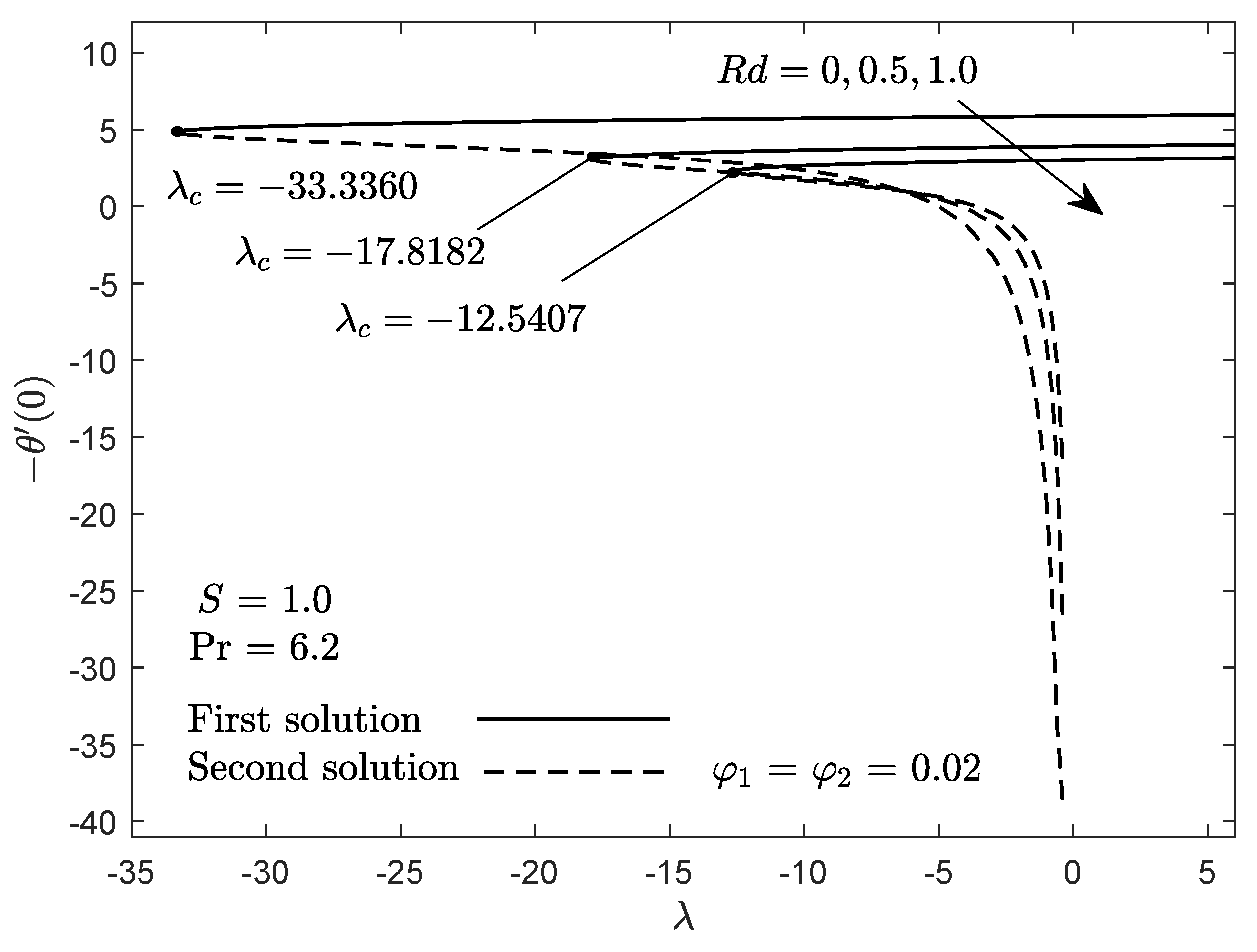
Figure 2 and Figure 3 demonstrate the surface shear stress and the local heat flux for both assisting ($\lambda >0$) and opposing ($\lambda <0$) flows and for several values of $Rd$ when $S=1.0$, ${\phi }_1={\phi }_2=0.02$ and $\mathrm{P}\mathrm{r}=6.2$. As depicted in the figures, larger $Rd$ gives lower values of $f^{″}\left(0\right)$ and $-{\theta }^{\prime }\left(0\right)$ compared to the case of no radiation ($Rd=0$). In addition, dual solutions exist when $\lambda <0$. Meanwhile, unique solutions are obtained when $\lambda >0$. Here, ${\lambda }_c$ represents a turning point where the first and second solutions intersect. Beyond the turning point ($\lambda <{\lambda }_c$), the similarity solutions terminate. As the values of $\lambda$ diminish from the positive (assisting flow) to negative (opposing flow) values, the shear stress and the local heat flux decrease for the first solution. In opposing flow, the buoyancy forces resist the fluid motion. Consequently, fluids in the boundary layer get retarded, acting as an adverse pressure gradient and reducing shear stress on the flat plate. Besides, assisting flow (heated plate) has a larger surface temperature compared to a fluid temperature, implying that the heat transfer takes place from the plate to the surrounding fluid.

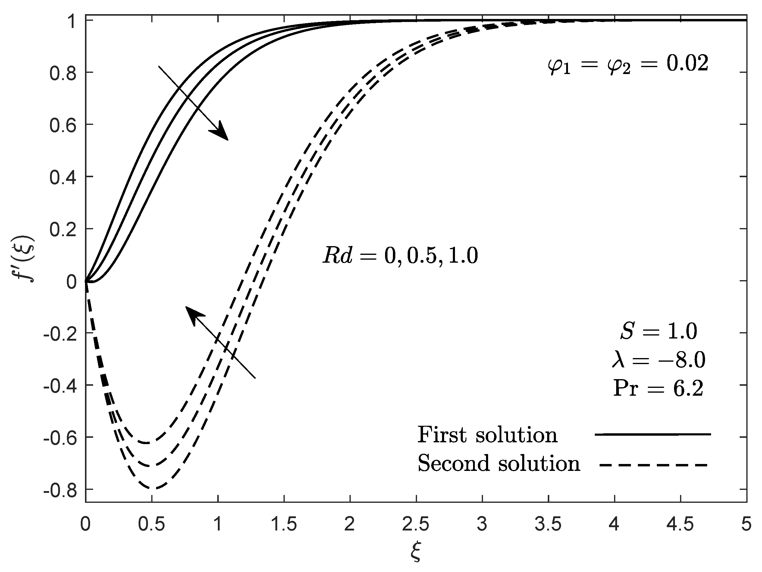
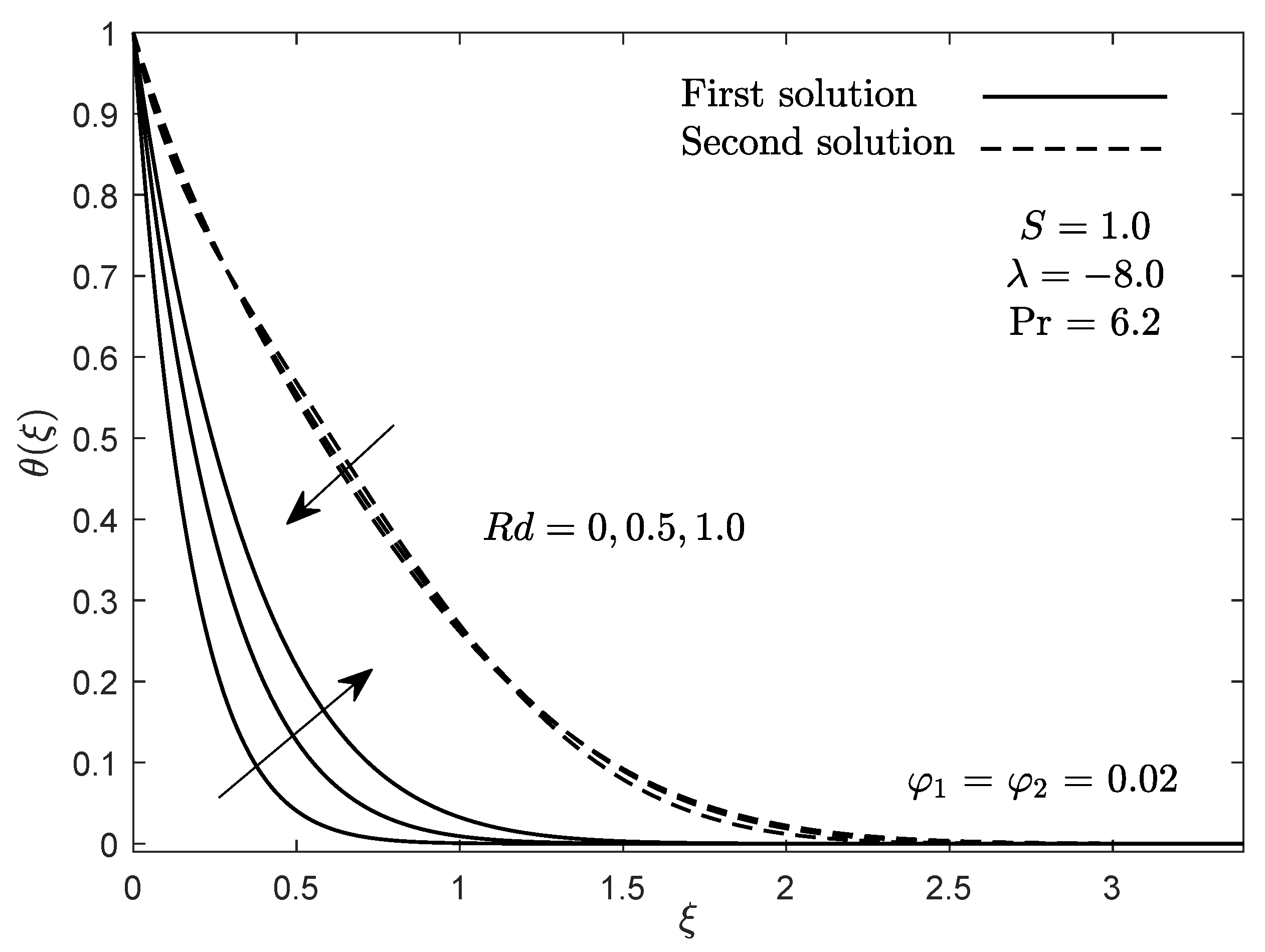
Figure 4 and Figure 5 illustrate the velocity and temperature distributions for various value of $Rd$ when $S=1.0$, $\lambda =-8.0$, ${\phi }_1={\phi }_2=0.02$ and $\mathrm{P}\mathrm{r}=6.2$. When $Rd$ gets larger, the momentum boundary layer thickness thickens (see Figure 4). This leads to a reduction in the velocity field. The opposite trend is observed for the temperature field, which increases as $Rd$ increases. Physically, radiation involves the emission or transmission of energy in the form of particles through a medium. Thus, increasing the parameter $Rd$ tends to enhance the temperature of the flow and its thermal layer thickness.

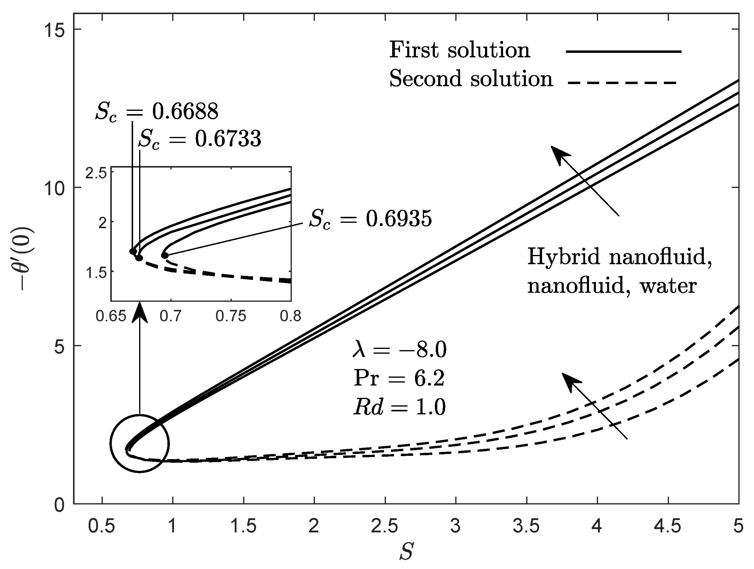
Figure 6 and Figure 7 present the values of $f^{″}\left(0\right)$ and $-{\theta }^{\prime }\left(0\right)$ for three different types of fluids namely, water $({\phi }_1={\phi }_2=0)$, nanofluid $({\phi }_1=0.02,{\phi }_2=0)$ and hybrid nanofluid $({\phi }_1={\phi }_2=0.02)$ with suction when $\lambda =-8.0$, $Rd=1.0$ and $\mathrm{P}\mathrm{r}=6.2$. The presence of a higher suction rate intensifies both values of $f^{″}\left(0\right)$ and $-{\theta }^{\prime }\left(0\right)$. This is due to the fact that the high suction rate accelerates the random motion of base fluid particles in the flow. This criterion leads to higher shear stress. The suction effect also speeds up the transportation of heat from the plate to the fluid. This happens due to the permeability of the plate itself. One can notice that water gives the largest shear stress and local heat flux compared to the others. Nanofluid and hybrid nanofluid contain more nanoparticles compared to water. Due to lack of space to collide, fluids with nanoparticles show a less favorable performance for shear stress formation. Besides, two solutions emerge when $S>S_c$. Meanwhile, no solutions exist when $S<S_c$.

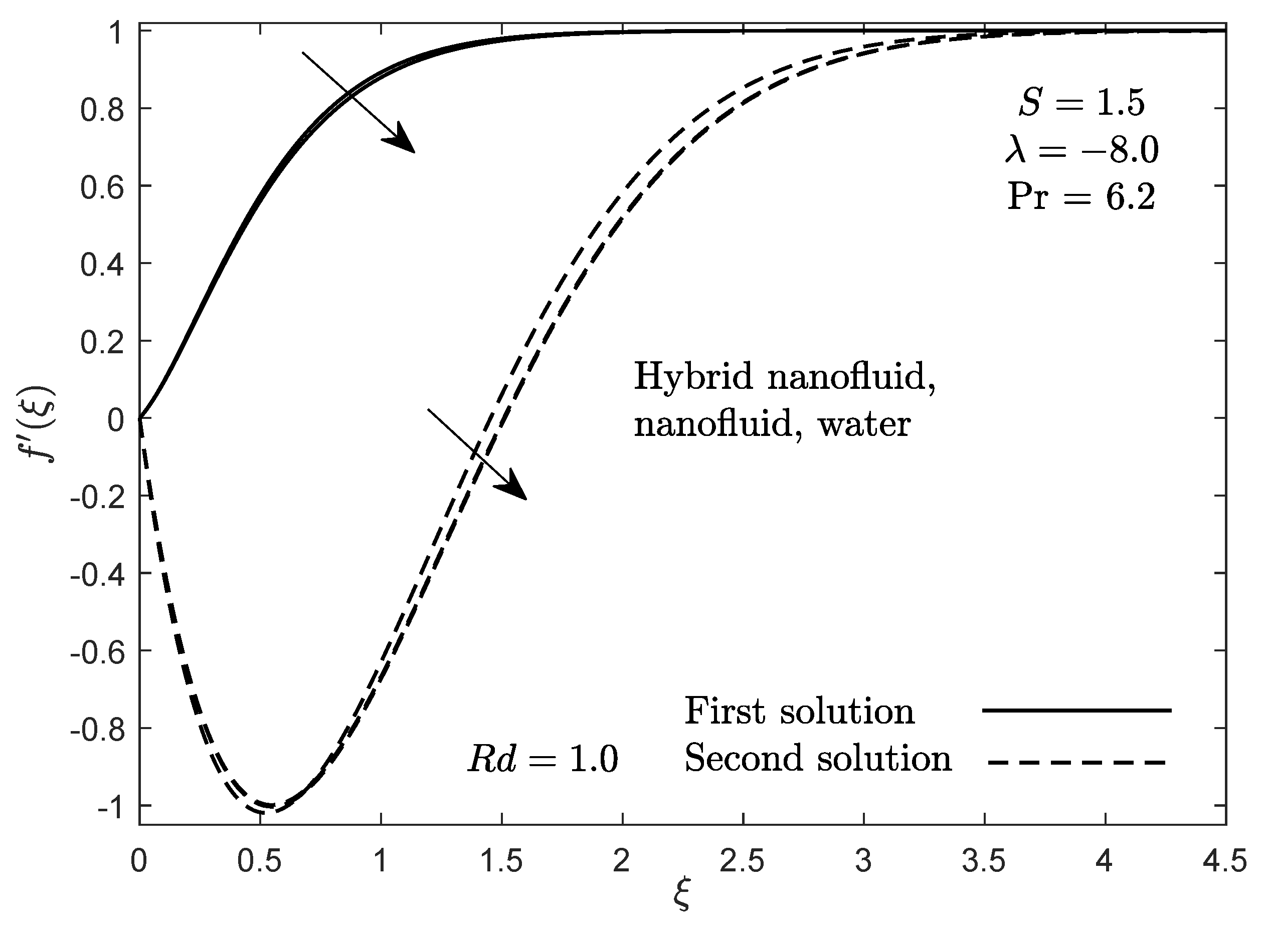
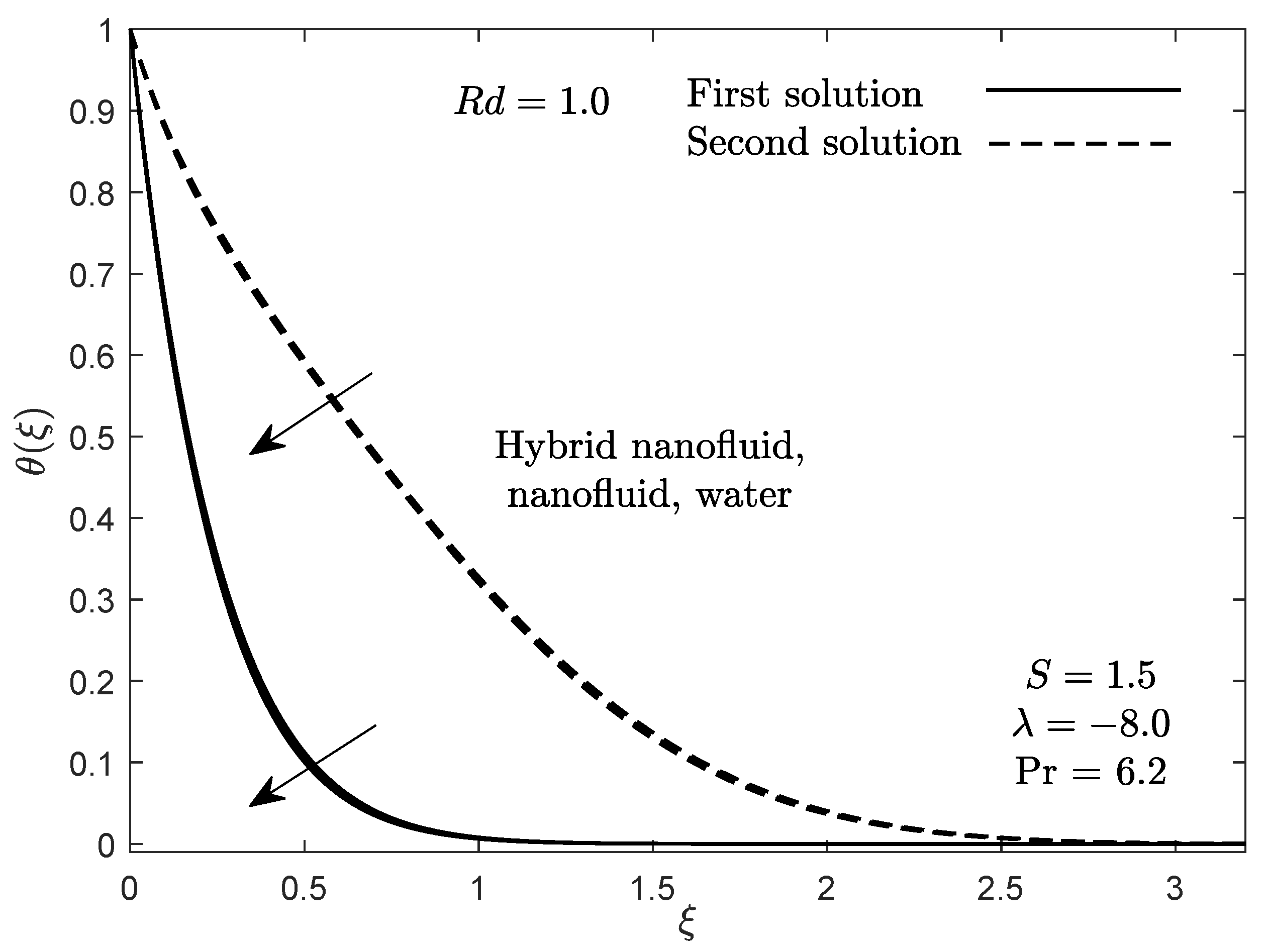
Figure 8 and Figure 9 demonstrate the velocity and temperature fields for several fluids when $\lambda =-8.0$, $Rd=1.0$, $S=1.5$ and $\mathrm{P}\mathrm{r}=6.2$. As depicted, hybrid nanofluid gives the larger velocity and temperature fields compared to others. The addition of more nanoparticles in the flow causes a continuous collision between the suspended particles (nanoparticles and base fluid particles). Thus, it enhances the velocity of the flow. Other than that, the number of suspended particles under the influence of radiation plays a vital role in temperature distributions. Increasing the number of particles in the system leads to high fluid temperatures.

Table 5. Values of $R{e}_x^{1/2}{C}_f$ and $R{e}_x^{-1/2}N{u}_x$ for $Rd$ and several types of fluids when $S=1.0$, $\lambda =-8.0$ and $\mathrm{P}\mathrm{r}=6.2$.

Physical Quantities	$\mathit{R}\mathit{d}$	Water	Nanofluid	Hybrid Nanofluid
$R{e}_x^{1/2}{C}_f$	0	0.812570	0.821348	0.848156
	0.5	0.274411	0.270165	0.241798
	1.0	−0.206219	−0.224329	−0.307333
$R{e}_x^{-1/2}N{u}_x$	0	6.478503	6.468462	6.483032
	0.5	6.681650	6.670055	6.683009
	1.0	6.802964	6.789484	6.794458

displays the skin friction coefficient ($R{e}_x^{1/2}{C}_f$) and the local Nusselt number ($R{e}_x^{-1/2}N{u}_x$) for some parameter $Rd$ and for several types of fluids. The table shows that the skin friction coefficients decline with larger $Rd$. In the case of no radiation $(Rd=0)$, hybrid nanofluid takes the largest value of $R{e}_x^{1/2}{C}_f$ and $R{e}_x^{-1/2}N{u}_x$. Meanwhile, in the presence of the radiation effect, water gives the largest skin friction coefficient. In addition to that, water exhibits the same behavior for the heat transfer rate when $Rd$ is high enough $(Rd=1)$. As the radiation rate intensifies, more heat is transferred in the form of nanoparticles. Besides, increasing the radiation rate from 0 (no radiation) to $1.0$ enhances the heat transfer rate by $5.01\%$ for water, $4.96\%$ for nanofluid, and $4.80\%$ for hybrid nanofluid. The main contribution of the radiation effect in this study is to enhance the thermal performance of the flow. Based on the results obtained, we have achieved the requirement for the cooling processes.

Table 6. Values of $R{e}_x^{1/2}{C}_f$ and $R{e}_x^{-1/2}N{u}_x$ for S and several types of fluids when $Rd=1.0$, $\lambda =-8.0$ and $\mathrm{P}\mathrm{r}=6.2$.

Physical Quantities	S	Water	Nanofluid	Hybrid Nanofluid
$R{e}_x^{1/2}{C}_f$	1	−0.206219	−0.224329	−0.307333
	2	1.395214	1.467937	1.632657
	3	2.609862	2.755097	3.115032
$R{e}_x^{-1/2}N{u}_x$	1	6.802964	6.789484	6.794458
	2	12.913871	12.868329	12.870270
	3	18.985538	18.902616	18.878203

presents the skin friction coefficient and the local Nusselt number for various values of S for several types of fluids. The values of S influence an increment in the skin friction coefficients. The presence of larger permeability of the plate accelerates the random motion of the suspended particles. As a result, they are increasing the friction on the boundary. Similarly, larger values of S tend to increase the heat transfer rate. Furthermore, water takes the largest skin friction coefficient when S is smaller ($S=1$). Nevertheless, when S increases from $S=2$ to $S=3$, hybrid nanofluid shows a prominent outcome compared to others.

Table 7. Minimum eigenvalues $\zeta$ for some values of $Rd$ and $\lambda$ when $S=1.0,{\phi }_1={\phi }_2=0.02$ and $\mathrm{P}\mathrm{r}=6.2$.

$\mathit{R}\mathit{d}$	$\mathit{\lambda }$	First Solution	Second Solution
0	−29.5378	1.2115	−1.0693
	−29.537	1.2117	−1.0694
	−29.53	1.2128	−1.0703
0.5	−17.0869	0.6463	−0.6034
	−17.086	0.6467	−0.6038
	−17.08	0.6494	−0.6061
1.0	−12.4563	0.2446	−0.2382
	−12.456	0.2450	−0.2386
	−12.45	0.2537	−0.2468

presents the minimum eigenvalues $\zeta$ of both solutions for some values of $Rd$ and $\lambda$. The positive value of $\zeta$ signifies that the first solution is stable, while the result is contrary to the second solution. In addition, as $\lambda$ approaches ${\lambda }_c$, the values of $\zeta$ continuously decreases until it approaches 0. Based on the previous studies on stability analysis [51], there exists an initial decline of disturbances in the region of the stable flow.

6. Conclusions

The analysis of mixed convection stagnation point flow in a hybrid nanofluid past a permeable flat surface has been investigated under the influence of radiation. The resulting system of equations is solved numerically via the bvp4c function in MATLAB software. The outcomes revealed that two solutions were obtained in the opposing flow region. The solutions terminated when $\lambda <{\lambda }_c$, where a unique solution was observed when $\lambda >0$. The stability analysis verified that the first solution is stable, whereas the second solution is unstable. The skin friction coefficient decreased with a larger radiation effect. Meanwhile, the heat transfer rate intensified with the radiation effect. Increasing the radiation rate from 0 (no radiation) to $1.0$ increased the heat transfer rate by $5.01\%$ for water, $4.96\%$ for nanofluid, and $4.80\%$ for hybrid nanofluid. Besides, the skin friction coefficient and the heat transfer rate were enhanced with a higher suction rate. In the absence of radiation effect, hybrid nanofluid produced higher values of $R{e}_x^{1/2}{C}_f$ and $R{e}_x^{-1/2}N{u}_x$. Meanwhile, in the presence of the radiation effect, water has the largest $R{e}_x^{1/2}{C}_f$ and $R{e}_x^{-1/2}N{u}_x$. The skin friction coefficient and the heat transfer rate increased with the suction effect for three types of fluids. Moreover, water produced the largest skin friction coefficient with smaller S ($S=1.0$). Meanwhile, hybrid nanofluid showed the prominent result for $R{e}_x^{1/2}{C}_f$ as S increased from $S=2$ to $S=3$. The significance of considering the radiation effect in this kind of flow is that it can reduce the skin friction coefficients for both assisting and opposing flows. Note that this criterion is good for the lubrication process. In addition, it can increase the heat transfer rate, which is suitable for certain applications that require high heat transfer rates (i.e., cooling processes).