Hybrid Inertial Accelerated Algorithms for Solving Split Equilibrium and Fixed Point Problems

Abstract

In this paper, we introduce a new hybrid inertial accelerated algorithm with a line search technique for solving fixed point problems for demimetric mapping and split equilibrium problems in Hilbert spaces. The algorithm is inspired by Tseng’s extragradient method and the viscosity method. Then, we establish and prove the strong convergence theorem under proper conditions. Furthermore, we also give a numerical example to support the main results. The main results are new and the proofs are relatively simple and different from those in early and recent literature.

1. Introduction

Let C be a nonempty, closed, and convex subset of a real Hilbert space $\mathcal{H}$ with scalar product $\langle ·,·\rangle$ and generated norm $∥·∥$. Let $F:C\times C\to \mathbb{R}$ be a bifunction. The Equilibrium Problem (EP) is of the form

$$\mathrm{find}\mathrm{a}\mathrm{point}u\in C\mathrm{such}\mathrm{that}F(u,v)\ge 0,\forall v\in C.$$

Denote the set of solutions of the EP as $\mathrm{EP}\left(F\right)$. The EP unifies many mathematical models such as the saddle point problems, the variational inequalities, and the optimization problems; see [1,2,3,4,5].

Given a mapping $B:C\to \mathcal{H}$, the Variational Inequality Problem (VIP) obtains a point $x^{*}\in C$ such that

$$\langle B{x}^{*},x-x^{*}\rangle \ge 0,\forall x\in C.$$

Solutions to these classes of problems, fixed point problems, and related optimization problems have been investigated and iterative algorithms for approximating them have been proposed and studied by several authors; see [6,7,8,9].

Let ${\mathcal{H}}_1$ and ${\mathcal{H}}_2$ be real Hilbert spaces, and let $C\subseteq {\mathcal{H}}_1$ and, $Q\subseteq {\mathcal{H}}_2$ be nonempty closed convex subsets. Let $F_1:C\times C\to \mathbb{R}$ and $F_2:Q\times Q\to \mathbb{R}$ be bifunctions. The Split Equilibrium Problem (SEP) finds

$$z\in C\mathrm{such}\mathrm{that}z\in \mathrm{EP}\left(F_1\right)\bigcap A^{-1}\left(\mathrm{EP}\left(F_2\right)\right),$$

where $A:{\mathcal{H}}_1\to {\mathcal{H}}_2$ is a bounded linear operator. Denote the set of solutions of the SEP as $\mathrm{SEP}(F_1,F_2)$. As we know, the SEP is a generalization of the EP by putting $F_2=0$ and $Q={\mathcal{H}}_2$. The SEP has been found to be useful in the study of many real-world problems such as data compression, sensor networks, medical reconstructions, etc. Additionally, the SEP is an extension of many mathematical models such as the split inclusion problem, the split feasibility problems, and the split variational inequality problems (SVIP, in which the solution set is denoted by SVIP(C,Q)); see [10,11,12] and the references therein.

In order to find a common solution for the fixed point problem for nonexpansive mapping and the SEP, Kazmi and Rizvi [12] suggested the following projection algorithm:

$$\left\{\begin{array}{c}{x}_{n+1}={\alpha }_{n}u+{\beta }_n{x}_n+{\gamma }_{n}S{y}_n,\hfill \\ y_n=P_C(u_n-{\lambda }_{n}T{u}_n),\hfill \\ u_n=T_{r_n}^{F_1}(x_n-\gamma A^{*}(I-T_{r_n}^{F_2})A{x}_n),n\ge 1,\hfill \end{array}\right.$$

where $S:C\to C$ is nonexpansive and $T:C\to {\mathcal{H}}_1$ is inverse strongly monotone. Then, the sequence $\left\{x_n\right\}$ converges strongly to an element in the solution set.

Recently, Jolaoso and Karahan [13] proposed the following general alternative regularization algorithm (Algorithm 1) for approximating a solution of the SEP and the fixed point for demicontractive mapping:

Algorithm 1: The general alternative regularization algorithm.

Initialization: Set $\zeta >0,l\in (0,1),\delta \in (0,1),\eta \in (0,2),$ and let $x_1\in {\mathcal{H}}_1$ be arbitrary. Step 1. Compute: $y_n=T_{r_n}^{F_1}(x_n-{\lambda }_n{A}^{*}(I-T_{r_n}^{F_2})A{x}_n)$, where ${\lambda }_n$ is chosen to be the largest $\gamma \in \{\zeta ,\zeta l,\zeta l^2,\zeta l^3,···\}$ satisfying the following: $$\gamma \langle A^{*}(I-T_{r_n}^{F_2})A{x}_n-A^{*}(I-T_{r_n}^{F_2})A{y}_n,x_n-y_n\rangle \le \delta {∥x_n-y_n∥}^2.$$ If $x_n=y_n$, then set $z_n=x_n$ and go to Step 3. Otherwise, do Step 2. Step 2. Compute: $$z_n=x_n-\eta d_n{e}_n,$$ where $$d_n=x_n-y_n-{\lambda }_n(A^{*}(I-T_{r_n}^{F_2})A{x}_n-A^{*}(I-T_{r_n}^{F_2})A{y}_n),$$ and $$e_n=(1-\delta )\frac{{∥x_n-y_n∥}^2}{{∥d_n∥}^2}.$$ Step 3. Compute $x_{n+1}=S_n({\alpha }_{n}f{z}_n+(1-{\alpha }_n)z_n)$, where $S_n=(1-{\eta }_n)I+{\eta }_{n}S.$ Set $n:=n+1$ and return to Step 1.

Assuming that $S:{\mathcal{H}}_1\to {\mathcal{H}}_1$ is a k-demicontractive mapping, $A:{\mathcal{H}}_1\to {\mathcal{H}}_2$ is a bounded linear operator with adjoint $A^{*}:{\mathcal{H}}_2\to {\mathcal{H}}_1$, $f:{\mathcal{H}}_1\to {\mathcal{H}}_1$ is Lipschitz and strongly pseudo-contractive, ${\eta }_n\in (0,1)$, and $0<{lim\; inf}_{n\to \infty }{\eta }_n\le {lim\; sup}_{n\to \infty }{\delta }_n<1-k$. Then, under certain appropriate assumptions, Algorithm 1 is to proven to converge strongly to the unique element.

On the other hand, in 2001, Alvarez and Attouch [14] used the heavy ball method that was studied in [15,16] for maximal monotone operators on the proximal point algorithm. The algorithm is said to be the inertial proximal point algorithm and it is as follows:

$$\left\{\begin{array}{c}{x}_{n+1}={(I+r_{n}T)}^{-1}{y}_n,\hfill \\ y_n=x_n+{\theta }_n(x_n-x_{n-1}),n\ge 1.\hfill \end{array}\right.$$

(1)

They also proved that the sequence $\left\{x_n\right\}$ constructed by (1) converges weakly to a zero of T under some suitable conditions.

Moreover, Cai et al. [17] proposed the following modified Tseng’s extragradient (Algorithm 2) for solving the pseudo-monotone variational inequality problem:

Algorithm 2: The new inertial Tseng’s extragradient iterative algorithm.

Initialization: Set $\zeta >0,l\in (0,1),\delta \in (0,1)$, and let $x_0,x_1\in \mathcal{H}$ be arbitrary. Step 1. Given $x_{n-1}$ and $x_n(n\ge 1)$, $n\ge 1$, compute $$u_n=x_n+{\mu }_n(x_n-x_{n-1}).$$ Step 2. Compute $y_n=P_C\left(u_n-{\lambda }_{n}A{u}_n\right)$, where ${\lambda }_n$ is chosen to be the largest $\gamma \in \{\zeta ,\zeta l,\zeta l^2,\zeta l^3,···\}$ satisfying the following: $$\begin{array}{c}\hfill \gamma ∥A{y}_n-A{u}_n∥\le \delta ∥u_n-y_n∥.\end{array}$$ If $u_n=y_n$ or $A{y}_n=0$, then stop. Otherwise, go to Step 3. Step 3. Compute $$z_n=y_n-{\lambda }_n\left(A{y}_n-A{u}_n\right).$$ Step 4. Compute $x_{n+1}={\alpha }_{n}f{x}_n+(1-{\alpha }_n)z_n$. Set $n:=n+1$ and return to Step 1.

Assume that $f:\mathcal{H}\to \mathcal{H}$ is contractive, $\left\{{\alpha }_n\right\}\subset (0,1)$, and $\left\{{\mu }_n\right\}$ is a sequence in $[0,1)$ satisfying ${lim}_{n\to \infty }\frac{{\mu }_n}{{\alpha }_n}∥x_n-x_{n-1}∥=0$. Then, they proved that the iterative sequence $\left\{x_n\right\}$ generated by Algorithm 2 converges to a solution of the pseudo-monotone variational inequality problem under some suitable conditions.

Motivated and inspired by Kazmi and Rizvi [12], Jolaoso and Karahan [13], Alvarez and Attouch [14], and Cai et al. [17], we suggest and analyze a hybrid inertial accelerated method for finding a common element of the set of fixed points of a demimetric mapping and the set of solutions of the split equilibrium problem in a real Hilbert space. We then prove a strong convergence of the proposed method under some mild conditions. Finally, we also provide a numerical experiment to demonstrate the efficiency of the proposed method over some existing ones.

2. Preliminaries

Throughout this paper, we denote the set of fixed points of a mapping T as $\mathrm{Fix}\left(T\right)$.

Lemma 1

([18]). In a real Hilbert space $\mathcal{H}$, the following hold:

(1) ${∥ku+(1-k)v∥}^2=k{∥u∥}^2+(1-k){∥v∥}^2-k(1-k){∥u-v∥}^2,\forall u,v\in \mathcal{H}$ and $k\in [0,1];$

(2)${∥u\pm v∥}^2={∥u∥}^2\pm 2\langle u,v\rangle +{∥v∥}^2,u,v\in \mathcal{H};$

(3) ${∥u+v∥}^2\le {∥u∥}^2+2\langle v,u+v\rangle ,u,v\in \mathcal{H}.$

Lemma 2

([19]). Let C be a nonempty closed convex subset of a real Hilbert space $\mathcal{H}$. For $u\in \mathcal{H}$ and $v\in C$, $v=P_{C}u$ if and only if

$$\langle u-v,w-v\rangle \le 0,\forall w\in C,$$

where $P_C$ is the metric projection from $\mathcal{H}$ onto C.

Definition 1.

A mapping $S:C\to \mathcal{H}$ is said to be

(1) 

nonexpansive, if

$$∥Su-Sv∥\le ∥u-v∥,\forall u,v\in C;$$

(2) 

γ-contractive, if there exists $\gamma \in [0,1)$ such that

$$∥Su-Sv∥\le \gamma ∥u-v∥,\forall u,v\in C;$$

(3) 

quasi-nonexpansive, if $\mathrm{Fix}\left(S\right)\ne \varnothing$ and

$$∥Su-x^{*}∥\le ∥u-x^{*}∥,\forall u\in C,x^{*}\in \mathrm{Fix}\left(S\right);$$

(4) 

α-strongly pseudo-contractive, if there exists a constant $\alpha \in [0,1)$, such that

$$\langle Su-Sv,u-v\rangle \le \alpha {∥u-v∥}^2,\forall u,v\in C;$$

(5) 

pseudo-monotone, if

$$\langle Sv,u-v\rangle \ge 0\Rightarrow \langle Su,u-v\rangle \ge 0,\forall u,v\in C;$$

(6) 

k-demicontractive, if $\mathrm{Fix}\left(S\right)\ne \varnothing$ and there exists $k\in [0,1)$, such that

$${∥Su-x^{*}∥}^2\le {∥u-x^{*}∥}^2+k{∥u-Su∥}^2,\forall u\in C,x^{*}\in \mathrm{Fix}\left(S\right);$$

(7) 

k-demimetric, if $\mathrm{Fix}\left(S\right)\ne \varnothing$ and there exists $k\in (-\infty ,1)$, such that

$${∥Su-x^{*}∥}^2\le {∥u-x^{*}∥}^2+k{∥u-Su∥}^2,\forall u\in C,x^{*}\in \mathrm{Fix}\left(S\right).$$

It is clear that the class of k-demimetric mappings contains the classes of k-demicontractive mappings. In 2017, Takahashi [20] also gave an example for a demimetric mapping that is not a demicontractive mapping, as follow:

Example 1

([20]). Let $\mathcal{H}$ be a real Hilbert spaces and C be a nonempty closed convex subsets of $\mathcal{H}$. Denote the metric projection of $\mathcal{H}$ onto C as $P_C$. Then, $P_C$ is (-1)-demimetric but $P_C$ is not demicontractive.

Assume that C is a nonempty, convex, and closed subset of a Hilbert space $\mathcal{H}$ and $F:C\times C\to \mathbb{R}$ is a bifunction satisfying the following restrictions:

(A1)

$F(u,u)=0$, $\forall u\in C$;

(A2)

F is monotone, i.e., $F(u,v)+F(v,u)\le 0$, $\forall u,v\in C$;

(A3)

For all $u,v,w\in C,$${lim\; sup}_{t\downarrow 0}F(tw+(1-t)u,v)\le F(u,v);$

(A4)

For all $u\in C,F(u,·)$ is convex and lower semicontinuous.

The following lemmas are needed.

Lemma 3

([21]). Let C be a nonempty closed convex subset of a real Hilbert space $\mathcal{H}$, and $T:C\to C$ be nonexpansive. Then, the mapping $I-T$ is demiclosed at zero, i.e., if $\left\{x_n\right\}$ converges weakly to a point $x\in C$ and $\{I-T)x_n\}$ converges to zero; then, $x=Tx$.

Lemma 4

([22,23]). Suppose that C is a nonempty close convex subset of a real Hilbert space $\mathcal{H}$. Assume that $S:C\to \mathcal{H}$ is k-demimetric such that $\mathrm{Fix}\left(S\right)$ is nonempty. Let κ be a real number with $\kappa \in (0,\infty )$, and define $T=(1-\kappa )I+\kappa S$. Then, it holds that

(1) 

$\mathrm{Fix}\left(T\right)=\mathrm{Fix}\left(S\right)$ if $\kappa \ne 0;$

(2) 

T is a quasi-nonexpansive mapping for $\kappa \in (0,1-k]$;

(3) 

$\mathrm{Fix}\left(S\right)$ is a closed convex subset of $\mathcal{H}$.

Lemma 5

([24]). Assume that $\left\{a_n\right\}$ is a sequence of real numbers such that there exists a subsequence $\left\{n_i\right\}$ of $\left\{n\right\}$ with $a_{n_i}<a_{n_i+1}$ for all $i\in \mathbb{N}$. Then, there exists a nondecreasing sequence $\left\{m_j\right\}\subseteq \mathbb{N}$ such that $m_j\to \infty$ and the following properties are satisfied for all (sufficiently large) numbers $j\in \mathbb{N}$:

$$a_{m_j}\le a_{m_j+1}\mathrm{and}{a}_j\le a_{m_j+1}.$$

Indeed, $m_j=max\{k\le j:a_k<a_{k+1}\}$.

Lemma 6

([25]). Assume that $\left\{a_n\right\}$ is a sequence of nonnegative numbers satisfying the following inequality:

$$a_{n+1}\le (1-{\beta }_n)a_n+{\gamma }_n+{\beta }_n{\delta }_n,n\in \mathbb{N},$$

where $\left\{{\beta }_n\right\},\left\{{\gamma }_n\right\},\left\{{\delta }_n\right\}$ satisfy the following restrictions:

(i) 

${\sum }_{n=1}^{\infty }{\beta }_n=\infty ,{lim}_{n\to \infty }{\beta }_n=0$,

(ii) 

${\gamma }_n\ge 0,{\sum }_{n=1}^{\infty }{\gamma }_n<\infty$,

(iii) 

${lim\; sup}_{n\to \infty }{\delta }_n\le 0$.

Then, ${lim}_{n\to \infty }{a}_n=0$.

Lemma 7

([26]). Assume that $F:C\times C\to \mathbb{R}$ satisfies (A1)–(A4). For $u\in \mathcal{H}$ and $r>0$, define a mapping $T_r^F:\mathcal{H}\to C$ as follows:

$$T_r^{F}u=\{w\in C:F(w,v)+\frac{1}{r}\langle v-w,w-u\rangle \ge 0,\forall v\in C\}.$$

Then, the following hold:

(i) 

$T_r^F$ is single-valued;

(ii) 

$T_r^F$ is a firmly nonexpansive mapping, i.e., for all $u,v\in H,$${∥T_r^{F}u-T_r^{F}v∥}^2\le \langle T_r^{F}u-T_r^{F}v,u-v\rangle ;$

(iii) 

$\mathrm{Fix}\left(T_r^F\right)=\mathrm{EP}\left(F\right);$

(iv) 

$\mathrm{EP}\left(F\right)$ is closed and convex.

3. Main Results

Let C and Q be nonempty convex closed subsets of real Hilbert spaces ${\mathcal{H}}_1$ and ${\mathcal{H}}_2$, respectively, and $A:{\mathcal{H}}_1\to {\mathcal{H}}_2$ be a bounded linear operator with adjoint $A^{*}:{\mathcal{H}}_2\to {\mathcal{H}}_1$. Assume that $F_1:C\times C\to \mathbb{R}$ and $F_2:Q\times Q\to \mathbb{R}$ are bifunctions satisfying assumptions (A1)–(A4). Assume that $S:{\mathcal{H}}_1\to {\mathcal{H}}_1$ is k-demimetric and that $I-S$ is demiclosed at zero. Let $f:{\mathcal{H}}_1\to {\mathcal{H}}_1$ be contractive with constant $\alpha \in (0,1).$ Assume that $\mathrm{Sol}:=\mathrm{SEP}(F1,F2)\bigcap \mathrm{Fix}\left(S\right)\ne \varnothing$ and that the following conditions are satisfied:

(C1)

$\left\{{\alpha }_n\right\}\subset (0,1)$, ${lim}_{n\to \infty }{\alpha }_n=0$ and ${\sum }_{n=1}^{\infty }{\alpha }_n=\infty$;

(C2)

$\left\{{\beta }_n\right\}\subset (0,1)$, $0<{lim\; inf}_{n\to \infty }{\beta }_n\le {lim\; sup}_{n\to \infty }{\beta }_n<1-k$;

(C3)

$\left\{{\mu }_n\right\}\subset [0,1]$ and ${lim}_{n\to \infty }\frac{{\mu }_n}{{\alpha }_n}∥x_n-x_{n-1}∥=0$, where $\left\{x_n\right\}$ is generated by Algorithm 3;

(C4)

$\left\{r_n\right\}\subset (0,\infty )$ and ${lim\; inf}_{n\to \infty }{r}_n>0$.

We now introduce the following algorithm:

Algorithm 3: The hybrid inertial accelerated algorithm.

Initialization: Set $\zeta >0,l\in (0,1),\delta \in (0,1)$ and let $x_0,x_1\in {\mathcal{H}}_1$ be arbitrary. Step 1. Given $x_{n-1}$ and $x_n(n\ge 1)$, compute $$u_n=x_n+{\mu }_n(x_n-x_{n-1}).$$ Step 2. Compute $y_n=T_{r_n}^{F_1}\left(u_n-{\lambda }_n{A}^{*}(I-T_{r_n}^{F_2})A{u}_n\right)$, where ${\lambda }_n$ is chosen to be the largest $\gamma \in \{\zeta ,\zeta l,\zeta l^2,\zeta l^3,···\}$ satisfying the following: $$\begin{array}{c}\hfill \gamma \parallel A^{*}(I-T_{r_n}^{F_2})A{y}_n-A^{*}(I-T_{r_n}^{F_2})A{u}_n\parallel \le \delta ∥u_n-y_n∥.\end{array}$$ (2) If $u_n=y_n$, then stop and $u_n$ is a solution of the SEP. Otherwise, Step 3. Compute $$z_n=y_n-{\lambda }_n\left(A^{*}(I-T_{r_n}^{F_2})A{y}_n-A^{*}(I-T_{r_n}^{F_2})A{u}_n\right).$$ Step 4. Compute $x_{n+1}=S_n\left({\alpha }_{n}f{x}_n+(1-{\alpha }_n)z_n\right)$, where $S_n=(1-{\beta }_n)I+{\beta }_{n}S.$ Set $n:=n+1$ and return to Step 1.

Before we prove the theorem, we need the following lemmas.

Lemma 8.

Suppose that $F:C\times C\to \mathbb{R}$ satisfies (A1)–(A4). For all $x\in \mathcal{H}$ and $0<a\le b$, the following inequality holds:

$$\begin{array}{c}\hfill \frac{a}{b}∥x-T_b^{F}x∥\le ∥x-T_a^{F}x∥\le ∥x-T_b^{F}x∥.\end{array}$$

Proof. 

Letting $x_a=T_a^{F}x$ and $x_b=T_b^{F}x$, we obtain

$$\begin{array}{c}\hfill F(x_a,y)+\frac{1}{a}\langle y-x_a,x_a-x\rangle \ge 0,\forall y\in C\end{array}$$

and

$$\begin{array}{c}\hfill F(x_b,y)+\frac{1}{b}\langle y-x_b,x_b-x\rangle \ge 0,\forall y\in C.\end{array}$$

Hence,

$$\begin{array}{c}\hfill F(x_a,x_b)+\frac{1}{a}\langle x_b-x_a,x_a-x\rangle \ge 0\end{array}$$

(3)

and

$$\begin{array}{c}\hfill F(x_b,x_a)+\frac{1}{b}\langle x_a-x_b,x_b-x\rangle \ge 0.\end{array}$$

(4)

Adding up (3) and (4) yields

$$\begin{array}{c}\hfill F(x_a,x_b)+F(x_b,x_a)+\langle x_a-x_b,\frac{x-x_a}{a}-\frac{x-x_b}{b}\rangle \ge 0.\end{array}$$

Noticing (A2), we have

$$\begin{array}{c}\hfill 0\le \langle x_a-x_b,\frac{x-x_a}{a}-\frac{x-x_b}{b}\rangle =\langle (x-x_b)-(x-x_a),\frac{x-x_a}{a}-\frac{x-x_b}{b}\rangle .\end{array}$$

This implies that

$$\begin{array}{c}\hfill 0\le -{∥x-x_a∥}^2-\frac{a}{b}{∥x-x_b∥}^2+(1+\frac{a}{b})∥x-x_a∥∥x-x_b∥.\end{array}$$

Therefore, we have

$$\begin{array}{c}\hfill (∥x-x_a∥-\frac{a}{b}∥x-x_b∥)(∥x-x_a∥-∥x-x_b∥)\le 0,\end{array}$$

which implies

$$\begin{array}{c}\hfill ∥x-x_a∥\ge \frac{a}{b}∥x-x_b∥\mathrm{and}∥x-x_a∥\le ∥x-x_b∥.\end{array}$$

Hence, we have

$$\begin{array}{c}\hfill \frac{a}{b}∥x-T_b^{F}x∥\le ∥x-T_a^{F}x∥\le ∥x-T_b^{F}x∥.\end{array}$$

   □

Lemma 9.

Assume that ${\mathcal{H}}_1$ and ${\mathcal{H}}_2$ are real Hilbert spaces, $A:{\mathcal{H}}_1\to {\mathcal{H}}_2$ is a linear operator with its adjoint $A^{*}$. For any $r>0$ and $x\in {\mathcal{H}}_1$, define a mapping $\tilde{T}:{\mathcal{H}}_1\to {\mathcal{H}}_1$ as $\tilde{T}:=A^{*}(I-T_r^F)A$. Then, the following statements hold:

(1) 

$∥\tilde{T}x-\tilde{T}y∥\le {∥A∥}^2∥x-y∥$;

(2) 

${∥(I-T_r^F)Ax-(I-T_r^F)Ay∥}^2\le \langle \tilde{T}x-\tilde{T}y,x-y\rangle$.

Proof. 

Since $T_r^F$ is a firmly nonexpansive mapping (Lemma 7(ii)), we deduce that $I-T_r^F$ is also firmly nonexpansive. Hence, we have that

$$\begin{array}{ccc}\hfill ∥\tilde{T}x-\tilde{T}y∥& \le & ∥A∥∥(I-T_r^F)Ax-(I-T_r^F)Ay∥\hfill \\ & \le & ∥A∥∥Ax-Ay∥\hfill \\ & \le & {∥A∥}^2∥x-y∥\hfill \end{array}$$

and

$$\begin{array}{ccc}\hfill {∥(I-T_r^F)Ax-(I-T_r^F)Ay∥}^2& \le & \langle Ax-Ay,(I-T_r^F)Ax-(I-T_r^F)Ay\rangle \hfill \\ & =& \langle x-y,A^{*}(I-T_r^F)Ax-A^{*}(I-T_r^F)Ay\rangle \hfill \\ & =& \langle x-y,\tilde{T}x-\tilde{T}y\rangle .\hfill \end{array}$$

   □

Lemma 10.

Assume that ${\mathcal{H}}_1$ and ${\mathcal{H}}_2$ are real Hilbert spaces, $A:{\mathcal{H}}_1\to {\mathcal{H}}_2$ is a linear operator with its adjoint $A^{*}$. Suppose that $\mathrm{SEP}(F1,F2)\ne \varnothing$ and $r>0.$ Then, the following statements hold:

(1) 

If $\widehat{x}$ is a solution of the $\mathrm{SEP}$, then $T_r^{F_1}\left(\widehat{x}-\lambda A^{*}(I-T_r^{F_2})A\widehat{x}\right)=\widehat{x}$;

(2) 

Assume that $T_r^{F_1}\left(\widehat{x}-\lambda A^{*}(I-T_r^{F_2})A\widehat{x}\right)=\widehat{x}$. Then, $\widehat{x}$ is a solution of the $\mathrm{SEP}$.

Proof. 

(1) Assume that $\widehat{x}\in {\mathcal{H}}_1$ is a solution of the $\mathrm{SEP}$. Then, $\widehat{x}\in \mathrm{EP}\left(F_1\right)$ and $A\widehat{x}\in \mathrm{EP}\left(F_2\right)$. By Lemma 7(iii), it is easy to see that

$$\begin{array}{c}\hfill T_r^{F_1}\left(\widehat{x}-\lambda A^{*}(I-T_r^{F_2})A\widehat{x}\right)=T_r^{F_1}\left(\widehat{x}\right)=\widehat{x}.\end{array}$$

(2) Suppose that the solution set of the $\mathrm{SEP}$ is nonempty and that $T_r^{F_1}\left(\widehat{x}-\lambda A^{*}(I-T_r^{F_2})A\widehat{x}\right)=\widehat{x}$. Then by Remark 1, we have

$$〈\left(\widehat{x}-\lambda A^{*}(I-T_r^{F_2})A\widehat{x}\right)-\widehat{x},z-\widehat{x}〉\le 0,\forall z\in \mathrm{EP}\left(F_1\right).$$

That is,

$$〈A^{*}(I-T_r^{F_2})A\widehat{x},\widehat{x}-z〉\le 0,\forall z\in \mathrm{EP}\left(F_1\right).$$

Thus, we obtain

$$〈A\widehat{x}-T_r^{F_2}A\widehat{x},A\widehat{x}-Az〉\le 0,\forall z\in \mathrm{EP}\left(F_1\right).$$

(5)

On the other hand, by Remark 1 again,

$$〈A\widehat{x}-T_r^{F_2}A\widehat{x},p-T_r^{F_2}A\widehat{x}〉\le 0,\forall p\in \mathrm{EP}\left(F_2\right).$$

(6)

Adding (5) and (6), we get

$$〈A\widehat{x}-T_r^{F_2}A\widehat{x},p-T_r^{F_2}A\widehat{x}+A\widehat{x}-Az〉\le 0,\forall z\in \mathrm{EP}\left(F_1\right),p\in \mathrm{EP}\left(F_2\right).$$

This implies

$${∥A\widehat{x}-T_r^{F_2}A\widehat{x}∥}^2\le 〈A\widehat{x}-T_r^{F_2}A\widehat{x},Az-p〉,\forall z\in \mathrm{EP}\left(F_1\right),p\in \mathrm{EP}\left(F_2\right).$$

(7)

Suppose that $\overline{z}\in {\mathcal{H}}_1$ is a solution of the $\mathrm{SEP}$. Then, $\overline{z}\in \mathrm{EP}\left(F_1\right)$ and $A\overline{z}\in \mathrm{EP}\left(F_2\right)$. Putting $z=\overline{z}$ and $p=A\overline{z}$ in (7), we deduce $A\widehat{x}\in \mathrm{Fix}\left(T_r^{F_2}\right)=\mathrm{EP}\left(F_2\right).$ Furthermore,

$$\begin{array}{c}\hfill \widehat{x}=T_r^{F_1}\left(\widehat{x}-\lambda A^{*}(I-T_r^{F_2})A\widehat{x}\right)=T_r^{F_1}\widehat{x}.\end{array}$$

Hence, $\widehat{x}\in \mathrm{Fix}\left(T_r^{F_1}\right)=\mathrm{EP}\left(F_1\right).$ Therefore, $\widehat{x}$ is a solution of the $\mathrm{SEP}$.    □

Remark 1.

By Lemma 7(ii), one can deduce (as in Remark 2.11 from Jolaoso and Karahan [13]) that, for any $u\in \mathcal{H}:$,

$$\langle T_r^{F}u-p,T_r^{F}u-u\rangle \le 0,\forall p\in \mathrm{Fix}\left(T_r^F\right).$$

Lemma 11.

The Armijo-like search rule (2) is well-defined and $min\{\zeta ,\delta l{∥A∥}^{-2}\}\le {\lambda }_n\le \zeta$.

Proof. 

Indeed, using Lemma 9(1), one sees that

$$\begin{array}{c}\hfill ∥A^{*}(I-T_{r_n}^{F_2})A{y}_n-A^{*}(I-T_{r_n}^{F_2})A{u}_n∥\le {∥A∥}^2∥y_n-u_n∥.\end{array}$$

Obviously, (2) holds for all $0<{\lambda }_n\le \delta {∥A∥}^{-2}$. On the other hand, it is easy to see that ${\lambda }_n\le \zeta$. If ${\lambda }_n=\zeta$; then, the lemma is proved. Otherwise, if ${\lambda }_n<\zeta ,$ then (2) will be violated when $\gamma ={\lambda }_n{l}^{-1}$, which indicates that ${\lambda }_n{l}^{-1}>\delta {∥A∥}^{-2}$. Hence, ${\lambda }_n\ge min\{\zeta ,\delta l{∥A∥}^{-2}\}$.    □

Lemma 12.

Suppose that Conditions (C1)–(C4) hold. Let $\left\{u_n\right\},\left\{y_n\right\}$, and $\left\{z_n\right\}$ be three sequences created by Algorithm 3. Then, for $\forall q\in \mathrm{SEP}(F1,F2)$,

$$\begin{array}{c}\hfill {∥z_n-q∥}^2\le {∥u_n-q∥}^2-(1-{\delta }^2){∥y_n-u_n∥}^2.\end{array}$$

Proof. 

Let $q\in \mathrm{SEP}(F1,F2)$, that is $T_{r_n}^{F_1}q=q$, $T_{r_n}^{F_2}Aq=Aq$. From the definitions of $z_n$, we find

$$\begin{array}{ccc}\hfill & & {∥z_n-q∥}^2\hfill \\ & =& {∥y_n-{\lambda }_n\left(A^{*}(I-T_{r_n}^{F_2})A{y}_n-A^{*}(I-T_{r_n}^{F_2})A{u}_n\right)-q∥}^2\hfill \\ & =& {∥y_n-q∥}^2+{\lambda }_n^2{∥A^{*}(I-T_{r_n}^{F_2})A{y}_n-A^{*}(I-T_{r_n}^{F_2})A{u}_n∥}^2\hfill \\ & & -2{\lambda }_n\langle y_n-q,A^{*}(I-T_{r_n}^{F_2})A{y}_n-A^{*}(I-T_{r_n}^{F_2})A{u}_n\rangle \hfill \\ & =& {∥y_n-u_n∥}^2+{∥u_n-q∥}^2+2\langle y_n-u_n,u_n-q\rangle +{\lambda }_n^2{∥A^{*}(I-T_{r_n}^{F_2})A{y}_n-A^{*}(I-T_{r_n}^{F_2})A{u}_n∥}^2\hfill \\ & & -2{\lambda }_n\langle y_n-q,A^{*}(I-T_{r_n}^{F_2})A{y}_n-A^{*}(I-T_{r_n}{y}^F)A{u}_n\rangle \hfill \\ & =& {∥y_n-u_n∥}^2+{∥u_n-q∥}^2-2\langle y_n-u_n,y_n-u_n\rangle +2\langle y_n-u_n,y_n-q\rangle \hfill \\ & & +{\lambda }_n^2{∥A^{*}(I-T_{r_n}^{F_2})A{y}_n-A^{*}(I-T_{r_n}^{F_2})A{u}_n∥}^2-2{\lambda }_n\langle y_n-q,A^{*}(I-T_{r_n}^{F_2})A{y}_n-A^{*}(I-T_{r_n}^{F_2})A{u}_n\rangle \hfill \end{array}$$

$$\begin{array}{ccc}\hfill & =& {∥u_n-q∥}^2-{∥y_n-u_n∥}^2+2\langle y_n-u_n+{\lambda }_n{A}^{*}(I-T_{r_n}^{F_2})A{u}_n,y_n-q\rangle \hfill \\ & & -2{\lambda }_n\langle A^{*}(I-T_{r_n}^{F_2})A{y}_n,y_n-q\rangle +{\lambda }_n^2{∥A^{*}(I-T_{r_n}^{F_2})A{y}_n-A^{*}(I-T_{r_n}^{F_2})A{u}_n∥}^2.\hfill \end{array}$$

(8)

Apply Remark 1 to obtain

$$\begin{array}{c}\hfill \langle y_n-u_n+{\lambda }_n{A}^{*}(I-T_{r_n}^{F_2})A{u}_n,y_n-q\rangle \le 0.\end{array}$$

(9)

Noticing $Aq=T_{r_n}^{F_2}Aq$, we obtain from Lemma 9(2) that

$$\begin{array}{c}\hfill \langle A^{*}(I-T_{r_n}^{F_2})A{y}_n,y_n-q\rangle \ge 0.\end{array}$$

(10)

It follows from (2), (8), (9), and (10) that

$$\begin{array}{ccc}\hfill {∥z_n-q∥}^2& \le & {∥u_n-q∥}^2-{∥y_n-u_n∥}^2+{\lambda }_n^2{∥A^{*}(I-T_{r_n}^{F_2})A{y}_n-A^{*}(I-T_{r_n}^{F_2})A{u}_n∥}^2\hfill \\ & \le & {∥u_n-q∥}^2-{∥y_n-u_n∥}^2+{\delta }^2{∥y_n-u_n∥}^2\hfill \\ & =& {∥u_n-q∥}^2-(1-{\delta }^2){∥y_n-u_n∥}^2.\hfill \end{array}$$

The proof is completed.    □

Lemma 13.

Suppose that the sequences $\left\{u_n\right\}$ and $\left\{y_n\right\}$ are created by Algorithm 3. If $u_{n_k}\rightharpoonup z^{*}$ and ${lim}_{n\to \infty }∥u_n-y_n∥=0,$ then $z^{*}\in \mathrm{SEP}(F1,F2)$.

Proof. 

Taking any $q\in \mathrm{SEP}(F1,F2)$, we know that $T_{r_n}^{F_2}Aq=Aq$. This implies that $A^{*}(I-T_{r_n}^{F_2})Aq=0.$ By Lemma 9(2), we obtain that

$$\begin{array}{c}\hfill \langle A^{*}(I-T_{r_n}^{F_2})A{y}_n-A^{*}(I-T_{r_n}^{F_2})Aq,y_n-q\rangle \ge {∥(I-T_{r_n}^{F_2})A{y}_n∥}^2.\end{array}$$

This together with (9) and Lemma 9(1) implies

$$\begin{array}{ccc}\hfill {\lambda }_n{∥A{y}_n-T_{r_n}^{F_2}A{y}_n∥}^2& \le & {\lambda }_n\langle A^{*}(I-T_{r_n}^{F_2})A{y}_n-A^{*}(I-T_{r_n}^{F_2})Aq,y_n-q\rangle \hfill \\ & \le & {\lambda }_n\langle A^{*}(I-T_{r_n}^{F_2})A{y}_n-A^{*}(I-T_{r_n}^{F_2})Aq,y_n-q\rangle \hfill \\ & & -\langle y_n-(u_n-{\lambda }_n{A}^{*}(I-T_{r_n}^{F_2})A{u}_n),y_n-q\rangle \hfill \\ & =& \langle u_n-y_n-{\lambda }_n{A}^{*}(I-T_{r_n}^{F_2})A{u}_n+{\lambda }_n{A}^{*}(I-T_{r_n}^{F_2})A{y}_n,y_n-q\rangle \hfill \\ & \le & ∥u_n-y_n-{\lambda }_n{A}^{*}(I-T_{r_n}^{F_2})A{u}_n+{\lambda }_n{A}^{*}(I-T_{r_n}^{F_2})A{y}_n∥∥y_n-q∥\hfill \\ & \le & \left(∥u_n-y_n∥+{\lambda }_n∥A^{*}(I-T_{r_n}^{F_2})A{u}_n-A^{*}(I-T_{r_n}^{F_2})A{y}_n∥\right)∥y_n-q∥\hfill \\ & \le & (1+{\lambda }_n{∥A∥}^2)∥u_n-y_n∥∥y_n-q∥.\hfill \end{array}$$

Since $min\{\zeta ,\delta l{∥A∥}^{-2}\}\le {\lambda }_n\le \zeta$ and ${lim}_{n\to \infty }∥u_n-y_n∥=0,$ we find that ${lim}_{n\to \infty }∥A{y}_n-T_{r_n}^{F_2}A{y}_n∥=0.$ Moreover, by Lemma 7(ii), one can deduce

$$\begin{array}{ccc}\hfill ∥A{u}_n-T_{r_n}^{F_2}A{u}_n∥& \le & ∥A{u}_n-A{y}_n+(T_{r_n}^{F_2}A{y}_n-T_{r_n}^{F_2}A{u}_n)∥+∥A{y}_n-T_{r_n}^{F_2}A{y}_n∥\hfill \\ & \le & 2∥A∥∥u_n-y_n∥+∥A{y}_n-T_{r_n}^{F_2}A{y}_n∥.\hfill \end{array}$$

This indicates that

$$\begin{array}{c}\hfill \underset{n\to \infty }{lim}∥A{u}_n-T_{r_n}^{F_2}A{u}_n∥=0.\end{array}$$

(11)

Again using Lemma 7(ii) and the definition of $y_n$, we derive

$$\begin{array}{ccc}\hfill ∥y_n-T_{r_n}^{F_1}{u}_n∥& =& ∥T_{r_n}^{F_1}(u_n-{\lambda }_n{A}^{*}(I-T_{r_n}^{F_2})A{u}_n)-T_{r_n}^{F_1}{u}_n∥\hfill \\ & \le & ∥{\lambda }_n{A}^{*}(I-T_{r_n}^{F_2})A{u}_n∥\hfill \\ & \le & {\lambda }_n∥A∥∥A{u}_n-T_{r_n}^{F_2}A{u}_n∥,\hfill \end{array}$$

which together with (11) gives that ${lim}_{n\to \infty }∥y_n-T_{r_n}^{F_1}{u}_n∥=0$. From ${lim}_{n\to \infty }∥y_n-u_n∥=0$, one obtains ${lim}_{n\to \infty }∥u_n-T_{r_n}^{F_1}{u}_n∥=0$.

According to (C4), there exists a positive number r and some positive integer $N_0$ such that $0<r<r_n(\forall n\ge N_0).$ It follows from Lemma 8 that

$$\begin{array}{c}\hfill \underset{n\to \infty }{lim}∥u_n-T_r^{F_1}{u}_n∥\le \underset{n\to \infty }{lim}∥u_n-T_{r_n}^{F_1}{u}_n∥=0.\end{array}$$

This combining with Lemma 3, Lemma 7(ii), and $u_{n_k}\rightharpoonup z^{*}$ yields $z^{*}\in \mathrm{Fix}\left(T_r^{F_1}\right)=\mathrm{EP}\left(F_1\right)$. Due to the fact that A is a linear bounded operator and $u_{n_k}\rightharpoonup z^{*}$, we get

$$\begin{array}{c}\hfill A{u}_{n_k}\rightharpoonup A{z}^{*}.\end{array}$$

(12)

Using (11) and Lemma 8, we obtain

$$\begin{array}{c}\hfill \underset{n\to \infty }{lim}∥A{u}_n-T_r^{F_2}A{u}_n∥\le \underset{n\to \infty }{lim}∥A{u}_n-T_{r_n}^{F_2}A{u}_n∥=0.\end{array}$$

(13)

By (12), (13), Lemma 3, and Lemma 7(iii), we get $A{z}^{*}\in \mathrm{Fix}\left(T_r^{F_2}\right)=\mathrm{EP}\left(F_2\right)$. Thus, we deduce that $z^{*}\in \mathrm{SEP}(F1,F2).$ The proof is completed.    □

Theorem 2.

Assume that conditions (C1)–(C4) are satisfied. Then, the iterative sequence $\left\{x_n\right\}$ constructed by Algorithm 3 converges to q in the norm, where $q=P_{\mathrm{Sol}}fq.$

Remark 2.

We note that the condition (C3) can be easily implemented due to the fact that the value of $∥x_n-x_{n-1}∥$ is known before choosing ${\mu }_n$. Indeed, the parameter ${\mu }_n$ can be chosen such that

$${\mu }_n=\left\{\begin{array}{c}\omega ,x_n=x_{n-1},\hfill \\ \frac{{\xi }_n}{∥x_n-x_{n-1}∥},x_n\ne x_{n-1},\hfill \end{array}\right.$$

where $\omega \ge 0$ and $\left\{{\xi }_n\right\}$ is a positive sequence such that ${\xi }_n=o\left({\alpha }_n\right)$.

We now prove the Theorem 2.

Proof. 

First, we prove that the sequence $\left\{x_n\right\}$ is bounded. Taking any $q\in \mathrm{Sol}$, we infer from Lemma 12 that

$$\begin{array}{c}\hfill ∥z_n-q∥\le ∥u_n-q∥.\end{array}$$

(14)

In view of the definition of $u_n$, one deduces

$$\begin{array}{c}\hfill ∥u_n-q∥\le ∥x_n-q∥+{\mu }_n∥x_n-x_{n-1}∥.\end{array}$$

(15)

Invoking (C3), there exists a positive constant $M_1<\infty$ such that

$$\frac{{\mu }_n}{{\alpha }_n}∥x_n-x_{n-1}∥\le M_1.$$

From (14), (15), and Lemma 4, one obtains

$$\begin{array}{ccc}\hfill ∥x_{n+1}-q∥& =& ∥S_n\left({\alpha }_{n}f{x}_n+(1-{\alpha }_n)z_n\right)-q∥\hfill \\ & \le & ∥{\alpha }_n(f{x}_n-q)+(1-{\alpha }_n)(z_n-q)∥\hfill \\ & \le & {\alpha }_n∥f{x}_n-fq∥+{\alpha }_n∥fq-q∥+(1-{\alpha }_n)∥z_n-q∥\hfill \\ & \le & {\alpha }_n\alpha ∥x_n-q∥+{\alpha }_n∥fq-q∥+(1-{\alpha }_n)(∥x_n-q∥+{\mu }_n∥x_n-x_{n-1}∥)\hfill \\ & \le & (1-(1-\alpha ){\alpha }_n)∥x_n-q∥+{\alpha }_n∥fq-q∥+{\alpha }_n{M}_1\hfill \\ & \le & (1-(1-\alpha ){\alpha }_n)∥x_n-q∥+{\alpha }_n(1-\alpha )\frac{∥fq-q∥+M_1}{1-\alpha }\hfill \\ & \le & max\{∥x_n-q∥,\frac{∥fq-q∥+M_1}{1-\alpha }\}\hfill \\ & \le & \cdots \le max\{∥x_1-q∥,\frac{∥fq-q∥+M_1}{1-\alpha }\}.\hfill \end{array}$$

This implies that sequence $\left\{x_n\right\}$ is bounded. At the same time, using (14), (15), and the definition of $\left\{y_n\right\}$, one concludes that $\left\{z_n\right\}$, $\left\{y_n\right\}$, and $\left\{u_n\right\}$ are bounded. According to Lemma 1(3), we obtain

$$\begin{array}{ccc}\hfill {∥u_n-q∥}^2& =& {∥x_n-q+{\mu }_n(x_n-x_{n-1})∥}^2\hfill \\ & \le & {∥x_n-q∥}^2+2{\mu }_n\langle x_n-x_{n-1},u_n-q\rangle \hfill \\ & \le & {∥x_n-q∥}^2+2{\mu }_n∥x_{n-1}-x_n∥∥u_n-q∥\hfill \\ & \le & {∥x_n-q∥}^2+{\mu }_n∥x_{n-1}-x_n∥M_2,\hfill \end{array}$$

(16)

where $M_2={sup}_{n\ge 0}\left\{2∥u_n-q∥\right\}<\infty .$

It follows from Lemma 4, Lemma 12, and (16) that

$$\begin{array}{ccc}\hfill & & {∥x_{n+1}-q∥}^2\hfill \\ & =& {∥S_n({\alpha }_{n}f{x}_n+(1-{\alpha }_n)z_n)-q∥}^2\hfill \\ & \le & {∥{\alpha }_{n}f{x}_n+(1-{\alpha }_n)z_n-q∥}^2\hfill \\ & \le & {\alpha }_n{∥f{x}_n-q∥}^2+(1-{\alpha }_n){∥z_n-q∥}^2\hfill \\ & \le & {\alpha }_n{∥f{x}_n-q∥}^2+{∥u_n-q∥}^2-(1-{\delta }^2){∥y_n-u_n∥}^2,\hfill \\ & \le & {\alpha }_n{∥f{x}_n-q∥}^2+{∥x_n-q∥}^2+{\mu }_n∥x_{n-1}-x_n∥M_2-(1-{\delta }^2){∥y_n-u_n∥}^2,\hfill \\ & \le & {\alpha }_n{M}_3+{∥x_n-q∥}^2-(1-{\delta }^2){∥y_n-u_n∥}^2,\hfill \end{array}$$

(17)

where $M_3={sup}_{n\ge 1}\{{∥f{x}_n-q∥}^2+\frac{{\mu }_n}{{\alpha }_n}∥x_{n-1}-x_n∥M_2\}<\infty .$ Let us rewrite (17) as

$$\begin{array}{c}\hfill (1-{\delta }^2){∥y_n-u_n∥}^2\le {\alpha }_n{M}_3+{∥x_n-q∥}^2-{∥x_{n+1}-q∥}^2.\end{array}$$

(18)

Setting $g_n={\alpha }_{n}f{x}_n+(1-{\alpha }_n)z_n$ and using (14), (16), and Lemma 1(1), we infer

$$\begin{array}{ccc}& & {∥x_{n+1}-q∥}^2\hfill \\ & =& {∥((1-{\beta }_n)I+{\beta }_{n}S)g_n-q∥}^2\hfill \\ & =& (1-{\beta }_n){∥g_n-q∥}^2+{\beta }_n{∥S{g}_n-q∥}^2-{\beta }_n(1-{\beta }_n){∥g_n-S{g}_n∥}^2\hfill \\ & \le & ((1-{\beta }_n){∥g_n-q∥}^2+{\beta }_n({∥g_n-q∥}^2+k{∥g_n-S{g}_n∥}^2)-{\beta }_n(1-{\beta }_n){∥g_n-S{g}_n∥}^2\hfill \\ & =& {∥g_n-q∥}^2-{\beta }_n(1-{\beta }_n-k){∥g_n-S{g}_n∥}^2\hfill \\ & \le & {\alpha }_n{∥f{x}_n-q∥}^2+(1-{\alpha }_n){∥z_n-q∥}^2-{\beta }_n(1-{\beta }_n-k){∥g_n-S{g}_n∥}^2\hfill \\ & \le & {\alpha }_n{∥f{x}_n-q∥}^2+{∥x_n-q∥}^2+{\mu }_n∥x_{n-1}-x_n∥M_2-{\beta }_n(1-{\beta }_n-k){∥g_n-S{g}_n∥}^2.\hfill \end{array}$$

Thus,

$$\begin{array}{c}\hfill {\beta }_n(1-{\beta }_n-k){∥g_n-S{g}_n∥}^2\le {∥x_n-q∥}^2-{∥x_{n+1}-q∥}^2+{\alpha }_n{∥f{x}_n-q∥}^2+{\mu }_n∥x_{n-1}-x_n∥M_2.\end{array}$$

(19)

We next show the convergence of $\left\{∥x_n-q∥\right\}$ to zero by the following two cases:

Case 1. Assume that there exists $N_0\in \mathbb{N}$ such that the sequence ${\left\{∥x_n-q∥\right\}}_{n\ge N_0}$ is monotonously decreasing; then, ${lim}_{n\to \infty }∥x_n-q∥$ exists. From (C1) and putting n tending to infinity in (18), we derive that

$$\begin{array}{c}\hfill \underset{n\to \infty }{lim}∥y_n-u_n∥=0.\end{array}$$

(20)

It follows from (C1), (C3), and the definitions of $u_n$ that

$$\begin{array}{c}\hfill \underset{n\to \infty }{lim}∥u_n-x_n∥=\underset{n\to \infty }{lim}{\mu }_n∥x_n-x_{n-1}∥=0.\end{array}$$

(21)

By (C1), (C2), (C3), and (19), we obtain

$$\begin{array}{c}\hfill \underset{n\to \infty }{lim}∥g_n-S{g}_n∥=0.\end{array}$$

(22)

Due to the fact that $g_n={\alpha }_{n}f{x}_n+(1-{\alpha }_n)z_n$, we infer

$$\begin{array}{c}\hfill \underset{n\to \infty }{lim}∥g_n-z_n∥=\underset{n\to \infty }{lim}{\alpha }_n∥f{x}_n-z_n∥=0.\end{array}$$

(23)

Noticing $min\{\zeta ,\delta l{∥A∥}^{-2}\}\le {\lambda }_n\le \zeta$ and resorting to the definition of $z_n$, Lemma 9(1), and (20), one deduces that

$$\begin{array}{c}\hfill \underset{n\to \infty }{lim}∥z_n-y_n∥={\lambda }_n∥A^{*}(I-T_{r_n}^{F_2})A{y}_n-A^{*}(I-T_{r_n}^{F_2})A{u}_n∥\le \underset{n\to \infty }{lim}{\lambda }_n{∥A∥}^2∥y_n-u_n∥=0.\end{array}$$

(24)

Thanks to (20), (21) and (24), one infers that

$$\begin{array}{c}\hfill \underset{n\to \infty }{lim}∥z_n-x_n∥=0.\end{array}$$

(25)

Taking into consideration that

$$\begin{array}{ccc}\hfill ∥x_{n+1}-z_n∥& =& ∥((1-{\beta }_n)I+{\beta }_{n}S)g_n-z_n∥\hfill \\ & \le & (1-{\beta }_n)∥g_n-z_n∥+{\beta }_n(∥S{g}_n-g_n∥+∥g_n-z_n∥),\hfill \end{array}$$

we deduce from (22) and (23) that

$$\begin{array}{c}\hfill \underset{n\to \infty }{lim}∥x_{n+1}-z_n∥=0.\end{array}$$

(26)

Noticing $∥x_{n+1}-x_n∥\le ∥x_{n+1}-z_n∥+∥z_n-x_n∥$, this together with (25) and (26) implies

$$\begin{array}{c}\hfill \underset{n\to \infty }{lim}∥x_{n+1}-x_n∥=0.\end{array}$$

(27)

As $\left\{x_n\right\}$ is bounded, it indicates that there exists a subsequence $\left\{x_{n_k}\right\}$ of $\left\{x_n\right\}$ that converges weakly to some $z\in {\mathcal{H}}_1$ and

$$\underset{n\to \infty }{lim\; sup}\langle fq-q,x_n-q\rangle =\underset{k\to \infty }{lim}\langle fq-q,x_{n_k}-q\rangle =\langle fq-q,z-q\rangle .$$

According to (20), (21), and Lemma 13, we derive $z\in \mathrm{SEP}(F1,F2)$. By the assumption that $I-S$ is demiclosed and noticing that (22), (23), and (25), we deduce $z\in \mathrm{Fix}\left(S\right)$. Therefore, $z\in \mathrm{Sol}$. It is easy to see that $P_{\mathrm{Sol}}f$ is a contractive mapping. Banach’s Contraction Mapping Principle implies that $P_{\mathrm{Sol}}f$ has a unique fixed point, say, $q\in {\mathcal{H}}_1$ and namely, $q=P_{\mathrm{Sol}}fq$. It follows from Lemma 2 that

$$\begin{array}{c}\hfill \langle fq-q,y-q\rangle \le 0,\forall y\in \mathrm{Sol}.\end{array}$$

Therefore, we have

$$\underset{n\to \infty }{lim\; sup}\langle fq-q,x_n-q\rangle =\underset{k\to \infty }{lim}\langle fq-q,x_{n_k}-q\rangle =\langle fq-q,z-q\rangle \le 0.$$

This together with (27) implies that

$$\underset{n\to \infty }{lim\; sup}\langle fq-q,x_{n+1}-q\rangle \le 0.$$

(28)

It follows from (14), (16), Lemma 1(3), and Lemma 4 that

$$\begin{array}{ccc}\hfill & & {∥x_{n+1}-q∥}^2\hfill \\ & \le & {∥{\alpha }_{n}f{x}_n+(1-{\alpha }_n)z_n-q∥}^2\hfill \\ & =& {∥{\alpha }_n(f{x}_n-fq)+(1-{\alpha }_n)(z_n-q)+{\alpha }_n(fq-q)∥}^2\hfill \\ & \le & {∥{\alpha }_n(f{x}_n-fq)+(1-{\alpha }_n)(z_n-q)∥}^2+2{\alpha }_n\langle fq-q,x_{n+1}-q\rangle \hfill \\ & \le & {\alpha }_n{∥f{x}_n-fq∥}^2+(1-{\alpha }_n){∥z_n-q∥}^2+2{\alpha }_n\langle fq-q,x_{n+1}-q\rangle \hfill \\ & \le & {\alpha }_n\alpha {∥x_n-q∥}^2+(1-{\alpha }_n)({∥x_n-q∥}^2+{\mu }_n∥x_n-x_{n-1}∥M_2)+2{\alpha }_n\langle fq-q,x_{n+1}-q\rangle \hfill \\ & \le & (1-{\alpha }_n(1-\alpha )){∥x_n-q∥}^2+{\alpha }_n\left(\frac{{\mu }_n}{{\alpha }_n}∥x_n-x_{n-1}∥M_2\right)+2{\alpha }_n\langle fq-q,x_{n+1}-q\rangle .\hfill \end{array}$$

Thus, from (28), (C1), (C3), and Lemma 6, we conclude that $x_n\to q.$

Case 2. Assume that $\left\{∥x_n-q∥\right\}$ is not monotonously decreasing. Then, there exists a subsequence $\left\{∥x_{n_i}-q∥\right\}$ of $\left\{∥x_n-q∥\right\}$ such that

$$∥x_{n_i}-q∥<∥x_{n_i+1}-q∥,\forall i\in \mathbb{N}.$$

(29)

According to Lemma 5, there exists a nondecreasing sequence $\left\{m_k\right\}\subset \mathbb{N}$ such that

$$max\{∥x_{m_k}-q∥,∥x_k-q∥\}\le ∥x_{m_k+1}-q∥.$$

(30)

Following a similar argument as in Case I, it is easy to obtain

$$\begin{array}{c}\hfill \underset{k\to \infty }{lim}∥x_{m_k+1}-x_{m_k}∥=0\end{array}$$

(31)

We want to show that

$$\underset{k\to \infty }{lim\; sup}\langle f\left(q\right)-q,x_{m_k+1}-q\rangle \le 0,$$

(32)

where $q=P_{\mathrm{Sol}}fq$. Without loss of generality, there exists a subsequence $\left\{x_{m_{k_j}}\right\}$ of $\left\{x_{m_k}\right\}$ such that $x_{m_{k_j}}\rightharpoonup w$ for some $w\in {\mathcal{H}}_1$ and

$$\underset{k\to \infty }{lim\; sup}\langle f\left(q\right)-q,x_{m_k}-q\rangle =\underset{j\to \infty }{lim}\langle f\left(q\right)-q,x_{m_{k_j}}-q\rangle .$$

Like in Case 1, we can also obtain $\omega \in \mathrm{Sol}$. Thus, we have by Lemma 2 that

$$\begin{array}{cc}\hfill \underset{k\to \infty }{lim\; sup}\langle f\left(q\right)-q,x_{m_k}-q\rangle & =\underset{j\to \infty }{lim}\langle f\left(q\right)-q,x_{m_{k_j}}-q\rangle \hfill \\ \hfill & =\langle f\left(q\right)-P_{\mathrm{Sol}}f\left(q\right),w-P_{\mathrm{Sol}}f\left(q\right)\rangle \hfill \\ \hfill & \le 0.\hfill \end{array}$$

This together with (31) implies

$$\begin{array}{c}\hfill \underset{k\to \infty }{lim\; sup}\langle f\left(q\right)-q,x_{m_k+1}-q\rangle \le 0.\end{array}$$

Resorting to (14), (16), Lemma 1(3), and Lemma 4, one deduces that

$$\begin{array}{ccc}& & {∥x_{m_k+1}-q∥}^2\hfill \\ & =& {∥S_{m_k}\left({\alpha }_{m_k}f{x}_{m_k}+(1-{\alpha }_{m_k})z_{m_k}\right)-q∥}^2\hfill \\ & \le & {∥{\alpha }_{m_k}(f{x}_{m_k}-fq)+(1-{\alpha }_{m_k})(z_{m_k}-q)+{\alpha }_{m_k}(fq-q)∥}^2\hfill \\ & \le & {∥{\alpha }_{m_k}(f{x}_{m_k}-fq)+(1-{\alpha }_{m_k})(z_{m_k}-q)∥}^2+2{\alpha }_{m_k}\langle fq-q,x_{m_k+1}-q\rangle \hfill \\ & \le & {\alpha }_{m_k}{∥f{x}_{m_k}-fq∥}^2+(1-{\alpha }_{m_k}){∥z_{m_k}-q∥}^2+2{\alpha }_{m_k}\langle fq-q,x_{m_k+1}-q\rangle \hfill \\ & \le & {\alpha }_{m_k}\alpha {∥x_{m_k}-q∥}^2+(1-{\alpha }_{m_k}){∥u_{m_k}-q∥}^2+2{\alpha }_{m_k}\langle fq-q,x_{m_k+1}-q\rangle \hfill \\ & \le & {\alpha }_{m_k}\alpha {∥x_{m_k}-q∥}^2+(1-{\alpha }_{m_k})({∥x_{m_k}-q∥}^2+{\mu }_{m_k}∥x_{m_k}-x_{m_k-1}∥M_2)+2{\alpha }_{m_k}\langle fq-q,x_{m_k+1}-q\rangle \hfill \\ & \le & (1-{\alpha }_{m_k}(1-\alpha )){∥x_{m_k}-q∥}^2+{\alpha }_{m_k}\left(\frac{{\mu }_n}{{\alpha }_{m_k}}∥x_{m_k}-x_{m_k-1}∥M_2\right)+2{\alpha }_{m_k}\langle fq-q,x_{m_k+1}-q\rangle ,\hfill \end{array}$$

which yields that

$$\begin{array}{ccc}& & (1-\alpha ){\alpha }_{m_k}{∥x_{m_k+1}-q∥}^2\hfill \\ & \le & (1-{\alpha }_{m_k}(1-\alpha ))\left({∥x_{m_k}-q∥}^2-{∥x_{m_k+1}-q∥}^2\right)+{\alpha }_{m_k}\left(\frac{{\mu }_n}{{\alpha }_{m_k}}∥x_{m_k}-x_{n-1}∥M_2\right)\hfill \\ & & +2{\alpha }_{m_k}\langle fq-q,x_{m_k+1}-q\rangle .\hfill \end{array}$$

Noticing (29), we infer

$$\begin{array}{c}\hfill {∥x_{m_k+1}-q∥}^2\le \frac{1}{1-\alpha }\left(\frac{{\mu }_n}{{\alpha }_{m_k}}∥x_{m_k}-x_{n-1}∥M_2\right)+\frac{2}{1-\alpha }\langle fq-q,x_{m_k+1}-q\rangle .\end{array}$$

By applying (C1), (C3), and (32), we get

$$\begin{array}{c}\hfill \underset{k\to \infty }{lim}∥x_{m_k+1}-q∥=0.\end{array}$$

It thus follows from (30) that

$$\underset{k\to \infty }{lim}∥x_k-q∥=0.$$

From the above, one can conclude that the sequences constructed by Algorithm 3 converge strongly to $q\in \mathrm{Sol}$, which is the unique fixed point of the contractive mapping $P_{\mathrm{Sol}}f$. This completes the proof.    □

Remark 3.

Compared with the known results in the literature, our results are very different from those in the following aspects.

• The proofs of our main results are simple and different from those in early and recent literature manly due to Lemma 8. More precisely, Lemma 8 together with Lemma 13 presents an interesting and simple method to prove $u_n\to p\in \mathrm{SEP}(F1,F2)$ under the conditions $u_n\rightharpoonup p$ and $∥u_n-T_{r_n}^F{u}_n∥\to 0$.
• Theorem 2 extends, improves, and develops the corresponding results in [12,13,14,17] from finding a solution for the VIP, a solution for the the EP, or a common solution for the SEP and the fixed point problem for demicontractive mappings to finding a common solution for the SEP and the fixed point problem for demimetric mappings. Moreover, our proof is also different from the one used in those paper.
• The numerical results have shown the effectiveness and fast convergence of our iterative scheme over the iterative schemes in [12,13,14,17].

Corollary 1.

Assume that Conditions (C1)–(C4) are satisfied. Then, the sequence $\left\{x_n\right\}$ constructed by Algorithm 4 converges strongly to a point q, where $q=P_{\mathrm{SVIP}(C,Q)}fq.$

Algorithm 4: The hybrid inertial accelerated algorithm for the SVIP and the fixed point problem.

Initialization: Set $\zeta >0,l\in (0,1),\delta \in (0,1)$ and let $x_0,x_1\in {\mathcal{H}}_1$ be arbitrary. Step 1. Given $x_{n-1}$ and $x_n(n\ge 1)$, compute $$u_n=x_n+{\mu }_n(x_n-x_{n-1}).$$ Step 2. Compute $y_n=P_C\left(u_n-{\lambda }_n{A}^{*}(I-P_Q)A{u}_n\right)$, where ${\lambda }_n$ is chosen to be the largest $\gamma \in \{\zeta l,\zeta l^2,\zeta l^3,···\}$ satisfying the following: $$\begin{array}{c}\hfill \gamma ∥A^{*}(I-P_Q)A{y}_n-A^{*}(I-P_Q)A{u}_n∥\le \delta ∥u_n-y_n∥.\end{array}$$ If $u_n=y_n$, then stop and $u_n$ is a solution of the SVIP. Otherwise, Step 3. Compute $$z_n=y_n-{\lambda }_n\left(A^{*}(I-P_Q)A{y}_n-A^{*}(I-P_Q)A{u}_n\right).$$ Step 4. Compute $x_{n+1}=S_n\left({\alpha }_{n}f{x}_n+(1-{\alpha }_n)z_n\right)$, where $S_n=(1-{\beta }_n)I+{\beta }_{n}S.$ Set $n:=n+1$ and return to Step 1.

Proof. 

In Theorem 2, put $F_1(x,y)=0,\forall x,y\in C$ and $F_2(u,v)=0,\forall u,v\in Q$. Then we have that $T_{r_n}^{F_1}=P_C$ and $T_{r_n}^{F_2}=P_Q$ for all $n\in \mathbb{N}.$ Thus we obtain the desired result from Lemma 2 and Theorem 2.    □

4. Application to Split Minimization Problems

Let C be a nonempty, closed, and convex subset of a Hilbert space $\mathcal{H}$. The constrained convex minimization problem is to find a point $v^{*}\in C$ such that

$$\psi \left(v^{*}\right)=\underset{v\in C}{min}\psi \left(v\right),$$

(33)

where $\psi :C\to \mathbb{R}$ is a continuous differentiable function.

Lemma 14

([15,27]). A necessary condition of optimality for a point $v^{*}\in C$ to be a solution of the minimization problem (33) is that $v^{*}$ solves the inequality

$$\begin{array}{c}\hfill \langle \nabla \psi \left(v^{*}\right),u-v^{*}\rangle \ge 0,\forall u\in C.\end{array}$$

(34)

Equivalently, $v^{*}\in C$ solves the fixed point equation $v^{*}=P_C(v^{*}-\gamma \nabla \psi \left(v^{*}\right)),$ for every constant $\gamma >0$. If, in addition, ψ is convex, then the optimality condition (34) is also sufficient.

Setting $F(z,v)=\langle \nabla \psi \left(z\right),v-z\rangle$, we can easily deduce that $F(z,v)$ satisfies condition (A1)–(A4) and $\mathrm{Argmin}\left(\psi \right)=\mathrm{EP}\left(F\right).$ Define a resolvent operator $T_{\gamma }^{\nabla \psi }:\mathcal{H}\to C$ as

$$T_{\gamma }^{\nabla \psi }u=\{z\in C:\langle \nabla \psi \left(z\right),v-z\rangle +\frac{1}{\gamma }\langle v-z,z-u\rangle \ge 0,\forall v\in C\}.$$

From Lemma 7(iii), we get $\mathrm{Fix}\left(T_{\gamma }^{\nabla \psi }\right)=\mathrm{EP}\left(F\right)=\mathrm{Argmin}\left(\psi \right).$ Let us recall the split convex minimization problem (SCMP) as follows:

$$\mathrm{finding}{v}^{*}\in \mathrm{Argmin}\left({\psi }_1\right)\mathrm{such}\mathrm{that}A{v}^{*}\in \mathrm{Argmin}\left({\psi }_2\right),$$

(35)

where C and Q are nonempty convex closed subsets of real Hilbert spaces ${\mathcal{H}}_1$ and ${\mathcal{H}}_2$, respectively, ${\psi }_1:C\to \mathbb{R}$ and ${\psi }_2:Q\to \mathbb{R}$ are two proper convex differentiable functions, $A:{\mathcal{H}}_1\to {\mathcal{H}}_2$ is a bounded linear operator with adjoint $A^{*}:{\mathcal{H}}_2\to {\mathcal{H}}_1$. We denote the set of solutions of Problem (35) by $\mathrm{SCMP}({\psi }_1,{\psi }_2).$ By setting $T_r^{F_1}=T_r^{\nabla {\psi }_1}$ and $T_r^{F_2}=T_r^{\nabla {\psi }_2}$, we have the following theorem follows directly from Theorem 2.

Theorem 3.

Let C and Q be nonempty closed convex subsets of real Hilbert spaces ${\mathcal{H}}_1$ and ${\mathcal{H}}_2$, respectively. Assume that $A:{\mathcal{H}}_1\to {\mathcal{H}}_2$ is a bounded linear operator with adjoint $A^{*}:{\mathcal{H}}_2\to {\mathcal{H}}_1$, ${\psi }_1:C\to \mathbb{R}$ and ${\psi }_2:Q\to \mathbb{R}$ are proper convex differentiable functions. Suppose that $S:{\mathcal{H}}_1\to {\mathcal{H}}_1$ is k-demimetric such that $I-S$ is demiclosed at zero and that $f:{\mathcal{H}}_1\to {\mathcal{H}}_1$ is α-contractive with constant $\alpha \in (0,1).$ Suppose that the conditions (C1)–(C4) hold and $\mathrm{Sol}:=\mathrm{SCMP}({\psi }_1,{\psi }_2)\bigcap \mathrm{Fix}\left(S\right)\ne \varnothing$. Then, the iterative sequence $\left\{x_n\right\}$ constructed by Algorithm 3 converges to q in the norm, where $q=P_{\mathrm{Sol}}fq.$

Algorithm 5: The general alternative regularization algorithm.

Initialization: Set $\zeta >0,l\in (0,1),\delta \in (0,1)$ and let $x_0,x_1\in {\mathcal{H}}_1$ be arbitrary. Step 1. Given $x_{n-1}$ and $x_n(n\ge 1)$, compute $$u_n=x_n+{\mu }_n(x_n-x_{n-1}).$$ Step 2. Compute $y_n=T_{r_n}^{\nabla {\psi }_1}\left(u_n-{\lambda }_n{A}^{*}(I-T_{r_n}^{\nabla {\psi }_2})A{u}_n\right)$, where ${\lambda }_n$ is chosen to be the largest $\gamma \in \{\zeta l,\zeta l^2,\zeta l^3,···\}$ satisfying the following: $$\begin{array}{c}\hfill \gamma ∥A^{*}(I-T_{r_n}^{\nabla {\psi }_2})A{y}_n-A^{*}(I-T_{r_n}^{\nabla {\psi }_2})A{u}_n∥\le \delta ∥u_n-y_n∥.\end{array}$$ If $u_n=y_n$, then stop and $u_n$ is a solution of the $\mathrm{SCMP}$. Otherwise, Step 3. Compute $$z_n=y_n-{\lambda }_n\left(A^{*}(I-T_{r_n}^{\nabla {\psi }_2})A{y}_n-A^{*}(I-T_{r_n}^{\nabla {\psi }_2})A{u}_n\right).$$ Step 4. Compute $x_{n+1}=S_n\left({\alpha }_{n}f{x}_n+(1-{\alpha }_n)z_n\right)$, where $S_n=(1-{\beta }_n)I+{\beta }_{n}S.$ Set $n:=n+1$ and return to Step 1.

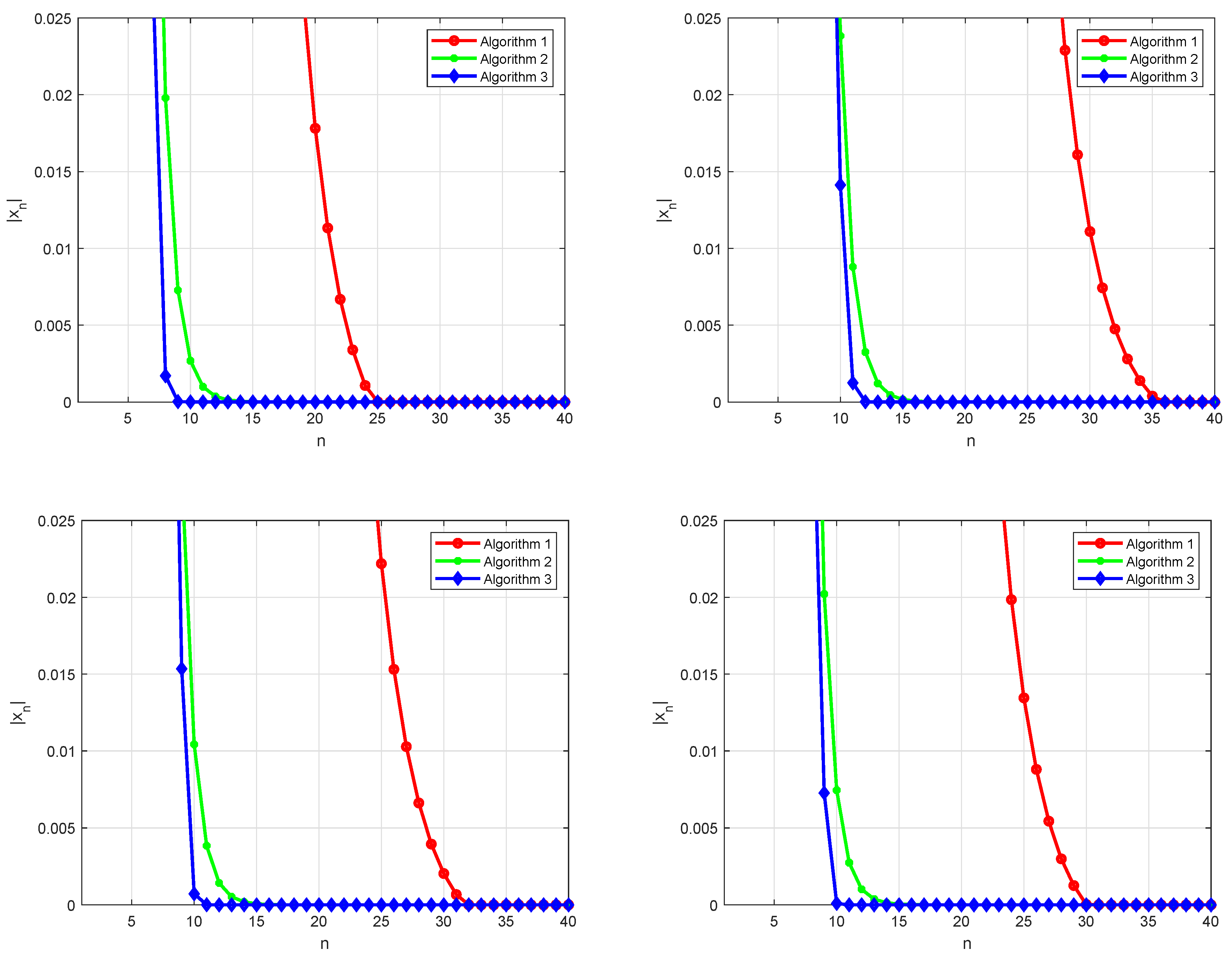
5. Numerical Examples

In this subsection, we discuss the numerical behavior of our proposed method in comparison with related methods in the literature. We compare Algorithm 3 with Algorithm 1 (Algorithm 3.1 of Jolaoso and Karahan [13]) and Algorithm 2 (Algorithm 2 of Cai et al. [17]).

Example 4.

Let ${\mathcal{H}}_1={\mathcal{H}}_2=\mathbb{R}$. Define $F_1:\mathbb{R}\times \mathbb{R}\to \mathbb{R}$ by $F_1(x,y)=-3x^2+xy+2y^2$ for all $x,y\in \mathbb{R}$ and $F_2:\mathbb{R}\times \mathbb{R}\to \mathbb{R}$ by $F_2(x,y)=-2x^2+xy+y^2$ for all $x,y\in \mathbb{R}$. It is easy to observe that $F_1$ and $F_2$ satisfy (A1)–(A4). By Lemma 7, it can be verified that $T_r^{F_1}x=\frac{x}{1+5r}$ and $T_r^{F_2}x=\frac{x}{1+3r}$. Let $f:\mathbb{R}\to \mathbb{R}$ be given by $fx=\frac{1}{2}x$, $A:\mathbb{R}\to \mathbb{R}$ be given by $Ax=2x$, and $S:\mathbb{R}\to \mathbb{R}$ be given by $Sx=\frac{1}{3}x$ for all $x\in \mathbb{R}$. We can easily deduce that f is a $\frac{1}{2}$-contraction, that A is a bounded linear operator, and that S is a 0-demimetric mapping. Additionally, it is not difficult to check that $\mathrm{Sol}=\left\{0\right\}.$ Let us choose ${\alpha }_n=\frac{1}{2n+1}$, ${\beta }_n=\frac{3}{4}$, ${\mu }_n=\frac{1}{2n^2+n}$, $\eta =\frac{10}{13}$, and $\delta =\zeta =l=\frac{1}{2}$. We test Algorithms 1–3 for different values of $x_0$ and $x_1$ as follows:

Case I: $x_0=100$ and $x_1=80$;

Case II: $x_0=50$ and $x_1=35$;

Case III: $x_0=30$ and $x_1=25$;

Case IV: $x_0=10$ and $x_1=9$.

We now compare the efficiency of Algorithm 3 with Algorithms 1 and 2. According to Figure 1,

Table 1. Numerical results for Example 4 in Case I.

Err	Algorithm 1		Algorithm 2		Algorithm 3
	$|{\mathit{x}}_{\mathit{n}}|$	$\mathit{n}$	$|{\mathit{x}}_{\mathit{n}}|$	$\mathit{n}$	$|{\mathit{x}}_{\mathit{n}}|$	$\mathit{n}$
${10}^{-3}$	1.0947111779190 $\times {10}^{-5}$	25	9.8932802287582 $\times {10}^{-4}$	11	2.5084018650195 $\times {10}^{-5}$	9
${10}^{-4}$	1.0947111779190 $\times {10}^{-5}$	25	5.0103649467704 $\times {10}^{-5}$	14	2.5084018650195 $\times {10}^{-5}$	9
${10}^{-5}$	1.0732462528617 $\times {10}^{-7}$	26	6.8899484598943 $\times {10}^{-6}$	16	3.3005287697625 $\times {10}^{-7}$	10

,

Table 2. Numerical results for Example 4 in Case II.

Err	Algorithm 1		Algorithm 2		Algorithm 3
	$|{\mathit{x}}_{\mathit{n}}|$	$\mathit{n}$	$|{\mathit{x}}_{\mathit{n}}|$	$\mathit{n}$	$|{\mathit{x}}_{\mathit{n}}|$	$\mathit{n}$
${10}^{-3}$	3.8495238046047 $\times {10}^{-4}$	36	5.5670721630783 $\times {10}^{-4}$	14	3.8440832718020 $\times {10}^{-5}$	12
${10}^{-4}$	2.6366601401402 $\times {10}^{-6}$	37	7.6554982887714 $\times {10}^{-5}$	16	3.8440832718020 $\times {10}^{-5}$	12
${10}^{-5}$	2.6366601401402 $\times {10}^{-6}$	37	3.9225807673322 $\times {10}^{-6}$	19	3.8440832718020 $\times {10}^{-7}$	13

,

Table 3. Numerical results for Example 4 in Case III.

Err	Algorithm 1		Algorithm 2		Algorithm 3
	$|{\mathit{x}}_{\mathit{n}}|$	$\mathit{n}$	$|{\mathit{x}}_{\mathit{n}}|$	$\mathit{n}$	$|{\mathit{x}}_{\mathit{n}}|$	$\mathit{n}$
${10}^{-3}$	6.7539211424883 $\times {10}^{-4}$	31	5.2608831941090 $\times {10}^{-4}$	13	7.1926227474796 $\times {10}^{-4}$	10
${10}^{-4}$	5.3602548749907 $\times {10}^{-6}$	32	7.2227962115800 $\times {10}^{-5}$	15	8.5626461279519 $\times {10}^{-6}$	11
${10}^{-5}$	5.3602548749907 $\times {10}^{-6}$	32	9.9463481554871 $\times {10}^{-6}$	17	8.5626461279519 $\times {10}^{-6}$	11

and

Table 4. Numerical results for Example 4 in Case IV.

Err	Algorithm 1		Algorithm 2		Algorithm 3
	$|{\mathit{x}}_{\mathit{n}}|$	$\mathit{n}$	$|{\mathit{x}}_{\mathit{n}}|$	$\mathit{n}$	$|{\mathit{x}}_{\mathit{n}}|$	$\mathit{n}$
${10}^{-3}$	3.0475500166712 $\times {10}^{-5}$	30	3.7577737100778 $\times {10}^{-4}$	13	9.5530385596659 $\times {10}^{-5}$	10
${10}^{-4}$	3.0475500166712 $\times {10}^{-5}$	30	5.1591401511286 $\times {10}^{-5}$	15	9.5530385596659 $\times {10}^{-5}$	10
${10}^{-5}$	2.4979918169436 $\times {10}^{-7}$	31	7.1045343967765 $\times {10}^{-6}$	17	1.1372664951983 $\times {10}^{-6}$	11

, one finds that Algorithm 3 has a better convergence behavior than Algorithms 1 and 2.

6. Conclusions

In this paper, we study a new iterative algorithm for solving split equilibrium problems and fixed point problems of demimetric mappings in Hilbert spaces. A theorem of strong convergence was proven under some mild conditions. The numerical behavior of the new algorithm is also studied by reporting a numerical experiment. In particular, it can be seen that the suggested algorithm has competitive advantages over some existing methods.

References

1. Blum, E.; Oettli, W. From optimization and variational inequalities to equilibrium problems. Math. Stud. 1994, 63, 123–145. [Google Scholar]
2. Cho, Y.J.; Petrot, N.; Suantai, S. Fixed point theorems for nonexpansive mappings with applications to generalized equilibrium and system of nonlinear variational inequalities problems. J. Nonl. Anal. Opt. 2010, 1, 45–53. [Google Scholar]
3. Yao, Y.; Cho, Y.J.; Liou, Y.C. Algorithms of common solutions for variational inclusions, mixed equilibrium problems and fixed point problems. Eur. J. Oper. Res. 2011, 212, 242–250. [Google Scholar] [CrossRef]
4. Tan, B.; Qin, X.; Yao, J.C. Strong convergence of self-adaptive inertial algorithms for solving split variational inclusion problems with applications. J. Sci. Comput. 2021, 87, 1–34. [Google Scholar] [CrossRef]
5. Tseng, P. A modified forward-backward splitting method for maximal monotone mappings. SIAM J. Control Optim. 2000, 38, 431–446. [Google Scholar] [CrossRef]
6. Alakoya, T.O.; Jolaoso, L.O.; Mewomo, O.T. A general iterative method for finding common fixed point of finite family of demicontractive mappings with accretive variational inequality problems in Banach spaces. Nonlinear Stud. 2020, 27, 1–24. [Google Scholar]
7. Ogwo, G.N.; Izuchukwu, C.; Mewomo, O.T. Inertial methods for finding minimum-norm solutions of the split variational inequality problem beyond monotonicity. Numer. Algorithms 2021. [Google Scholar] [CrossRef]
8. Chidume, C.E.; Maˇruşter, Şt. Iterative methods for the computation of fixed points of demicontractive mappings. J. Comput. Appl. Math. 2010, 234, 861–882. [Google Scholar] [CrossRef] [Green Version]
9. Cai, G.; Dong, Q.-L.; Peng, Y. Strong convergence theorems for solving variational inequality problems with pseudo-monotone and non-Lipschitz operators. J. Opt. Theory Appl. 2021, 188, 447–472. [Google Scholar] [CrossRef]
10. Censor, Y.; Bortfeld, T.; Martin, B.; Trofimov, A. A unified approach for inversion problem in intensity-modulated radiation therapy. Phys. Med. Biol. 2006, 51, 2353–2365. [Google Scholar] [CrossRef] [Green Version]
11. Ansari, Q.H.; Rehan, A. Split feasibility and fixed point problems. In Nonlinear Analysis: Approximation Theory, Optimization and Application; Ansari, Q.H., Ed.; Springer: New York, NY, USA, 2014; pp. 281–322. [Google Scholar]
12. Kazmi, K.R.; Rizvi, S.H. Iterative approximation of a common solution of a split equilibrium problem, a variational inequality problem and a fixed point problem. J. Egypt. Math. Soc. 2013, 21, 44–51. [Google Scholar] [CrossRef] [Green Version]
13. Jolaoso, L.O.; Karahan, I. A general alternative regularization method with line search technique for solving split equilibrium and fixed point problems in Hilbert spaces. Comput. Appl. Math. 2020, 39, 1–22. [Google Scholar] [CrossRef]
14. Alvarez, F.; Attouch, H. An inertial proximal method for monotone operators via discretization of a nonlinear oscillator with damping. Set-Valued Anal. 2001, 9, 3–11. [Google Scholar] [CrossRef]
15. Polyak, B.T. Introduction to Optimization; Optimization Software: New York, NY, USA, 1987. [Google Scholar]
16. Polyak, B.T. Some methods of speeding up the convergence of iterarive methods. Z. Vychisl. Mat. Mat. Fiz. 1964, 4, 1–17. [Google Scholar]
17. Cai, G.; Shehu, Y.; Iyiola, O.S. Inertial Tseng’s extragradient method for solving variational inequality problems of pseudo-monotone and non-Lipschitz operators. J. Ind. Manag. Optim. 2021. [Google Scholar] [CrossRef]
18. Takahashi, W. Introduction to Nonlinear and Convex Analysis; Yokohama Publishers: Yokohama, Japan, 2009. [Google Scholar]
19. Marino, G.; Xu, H.K. Weak and strong convergence theorems for strict pseudo-contractions in Hilbert spaces. J. Math. Anal. Appl. 2007, 329, 336–349. [Google Scholar] [CrossRef] [Green Version]
20. Takahashi, W. The split common fixed point problem and the shrinking projection method in banach spaces. J. Convex Anal. 2017, 24, 1015–1028. [Google Scholar]
21. Browder, F.E. Convergence of approximants to fixed points of nonexpansive nonlinear mappings in Banach spaces. Arch. Ration. Mech. Anal. 1967, 24, 82–90. [Google Scholar] [CrossRef]
22. Takahashi, W.; Wen, C.F.; Yao, J.C. The shrinking projection method for a finite family of demimetric mappings with variational inequality problems in a Hilbert space. Fixed Point Theory 2018, 19, 407–420. [Google Scholar] [CrossRef]
23. Song, Y. Iterative methods for fixed point problems and generalized split feasibility problems in Banach spaces. J. Nonl. Sci. Appl. 2018, 11, 198–217. [Google Scholar] [CrossRef] [Green Version]
24. Maingé, P.E. The viscosity approximation process for quasi-nonexpansive mappings in Hilbert spaces. Comput. Math. Appl. 2010, 59, 74–79. [Google Scholar] [CrossRef] [Green Version]
25. Xu, H.K. Iterative algorithm for nonlinear operators. J. Lond. Math. Soc. 2002, 2, 1–17. [Google Scholar] [CrossRef]
26. Combettes, P.L. Hirstoaga, S.A. Equilibrium programming in Hilbert spaces. J. Nonlinear Convex Anal. 2005, 6, 117–136. [Google Scholar]
27. Su, M.; Xu, H.-K. Remarks on the gradient-projection algorithm. J. Nonlinear Anal. Optim. 2010, 1, 35–43. [Google Scholar]
Figure 1. (Top left) Case I; (top right) Case II, (bottom left) Case III, (bottom right) Case IV.
Mathematics 09 02680 g001