
A Fully Resolved Computational Fluid Dynamics Study of the Boundary Layer Flow of an Aqueous Nanoliquid Comprising Gyrotactic Microorganisms over a Stretching Sheet: The Validity of Conventional Similarity Models

 , and
, and
Abstract
:1. Introduction
2. Materials and Methods
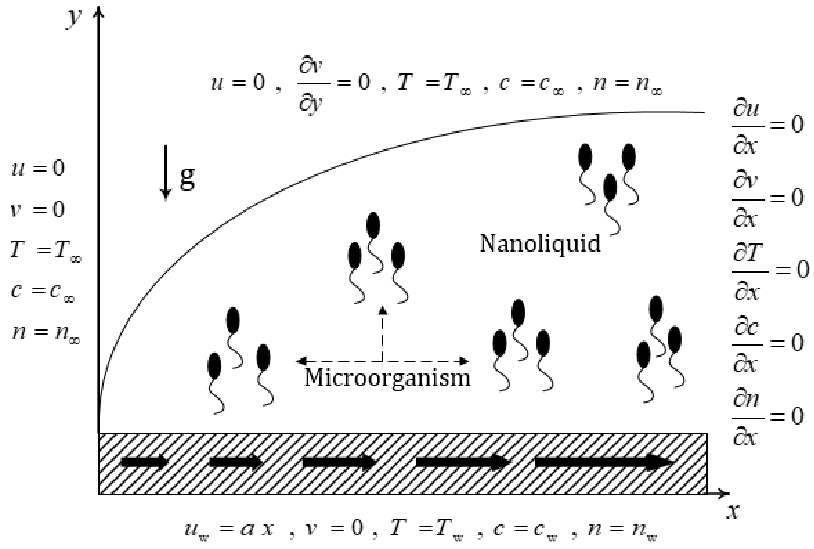
2.1. Problem Formulation
- The flow is incompressible, viscous, steady, and laminar.
- The sheet is impermeable.
- There is no slip on the sheet surface.
- The nanoliquid is dilute so the nanoparticles do not interact with each other or affect the motion of the microorganisms.
- The Boussinesq approximation may be applied to any change in density.
- The Brownian motion and thermophoresis are considered.
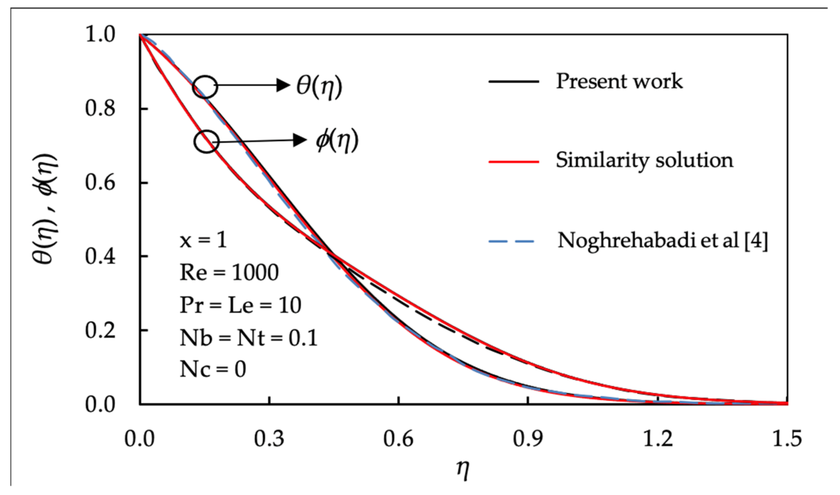
2.2. Numerical Approach, Mesh Sensitivity Analysis, and Validity
3. Results and Discussion
4. Conclusions
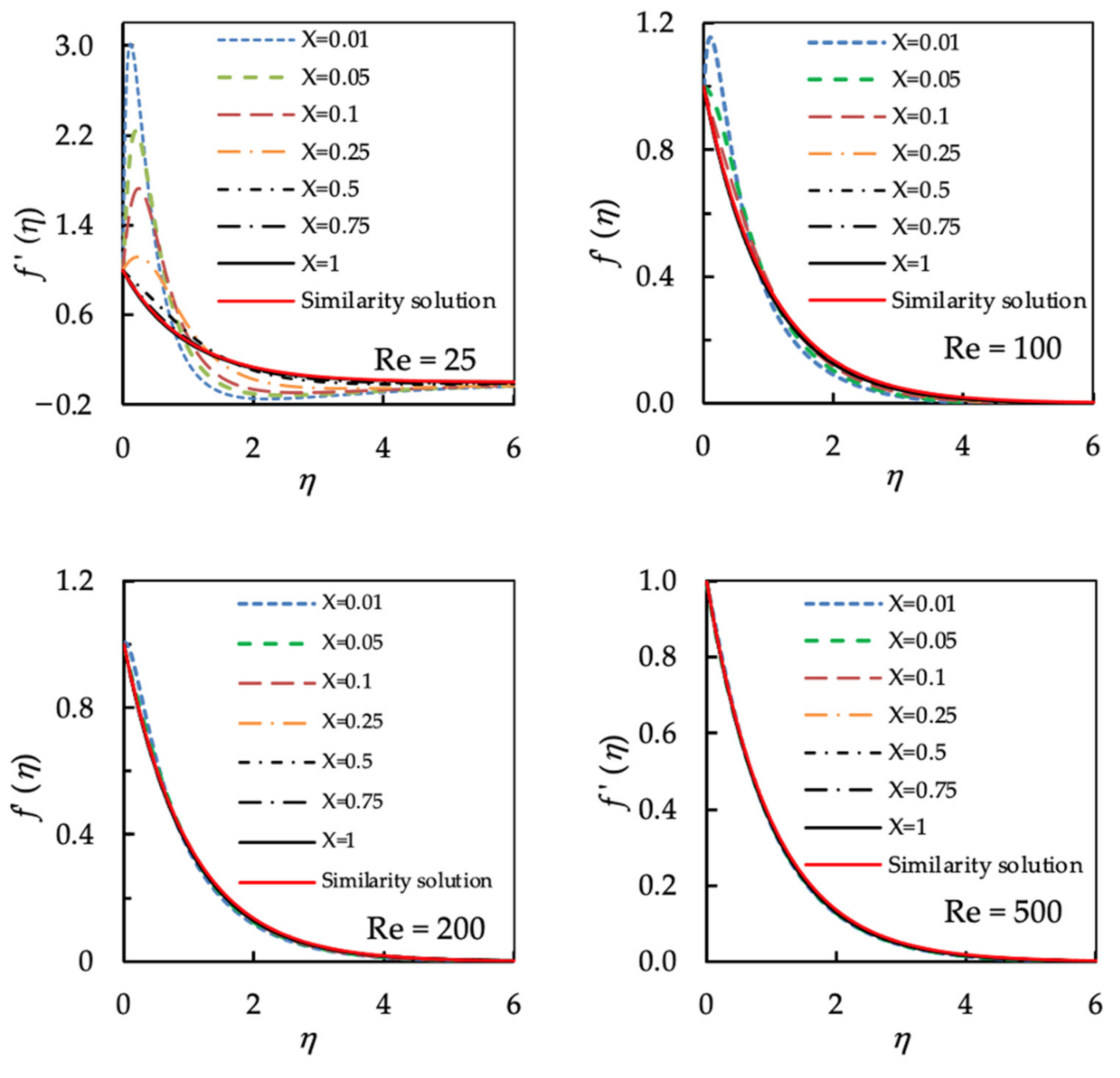
- At low values of Reynolds numbers (Re = 25 and Re = 100), the velocity experienced an overshoot in the vicinity of the extrusion slit. However, the maximum velocity occurred at the sheet surface when the Reynolds number was high.
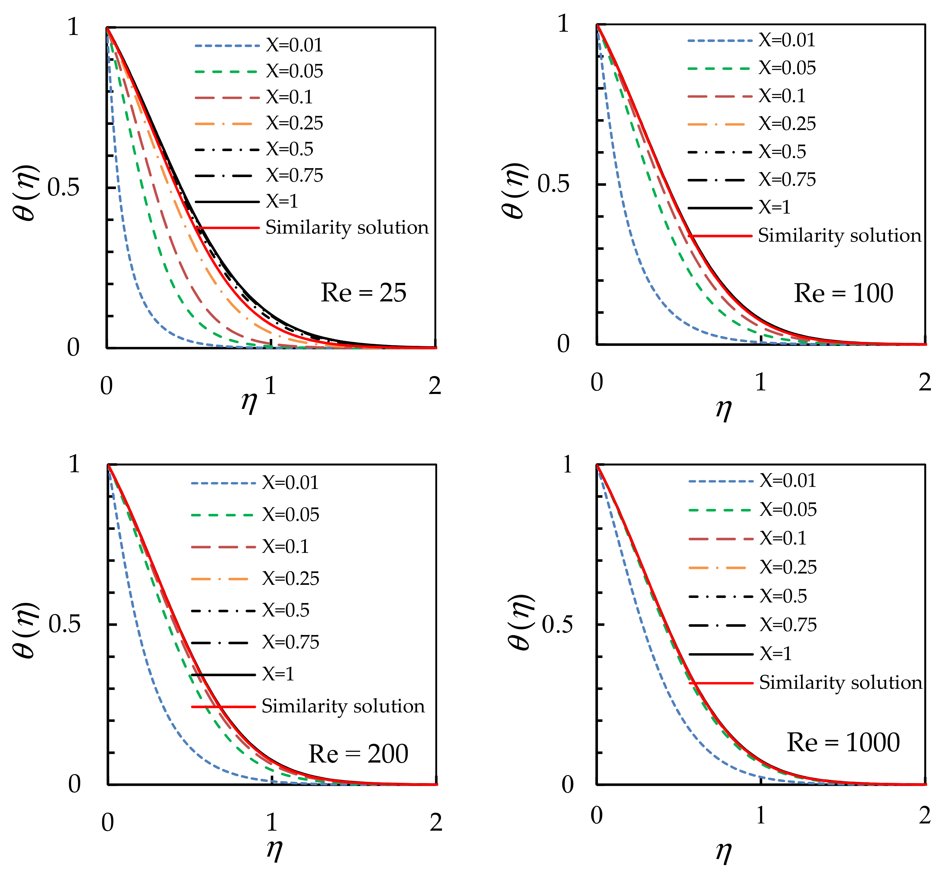
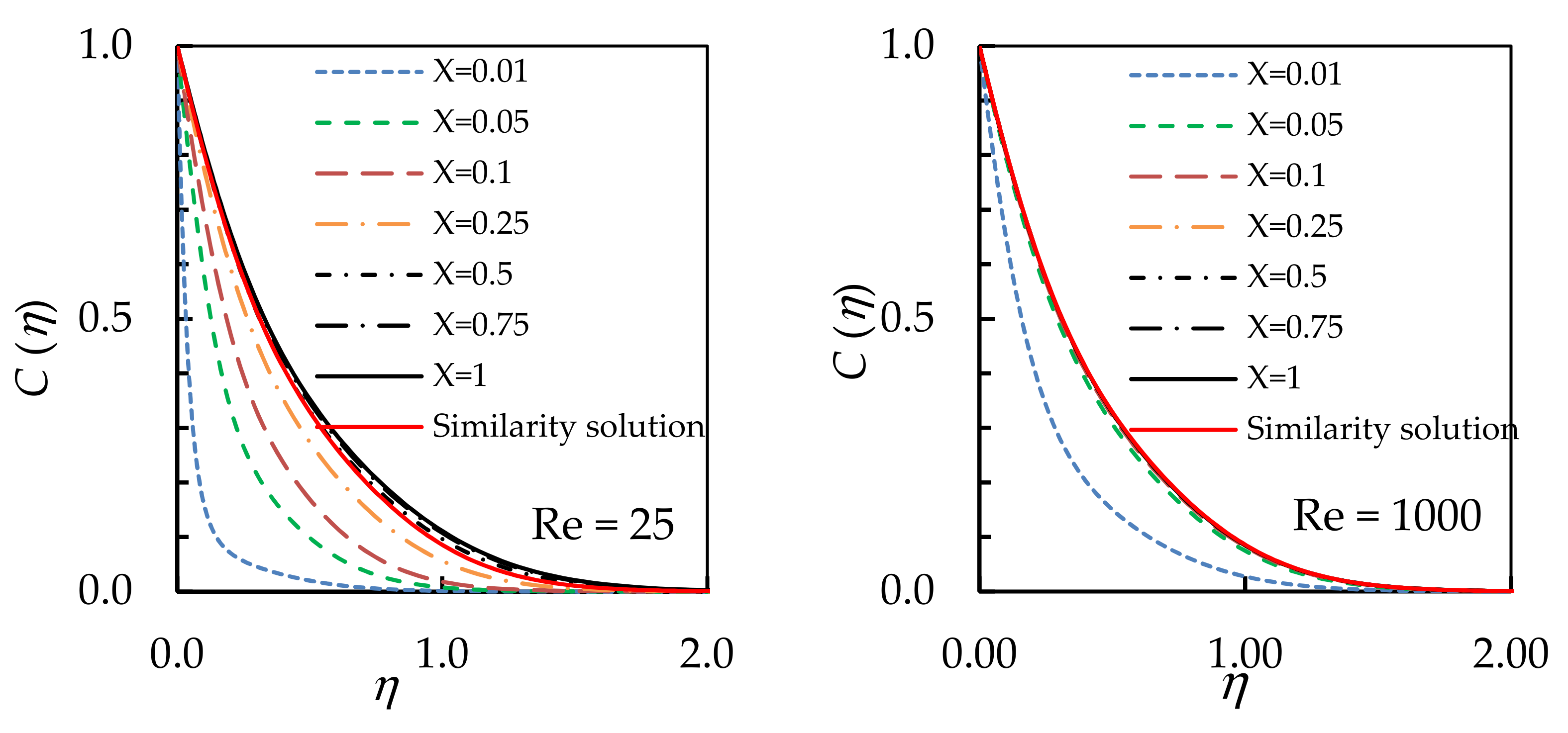
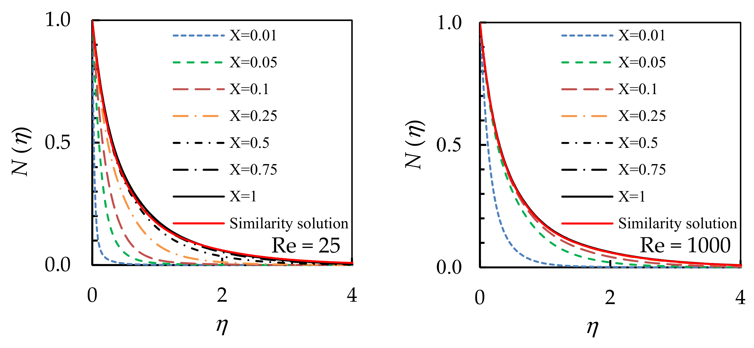
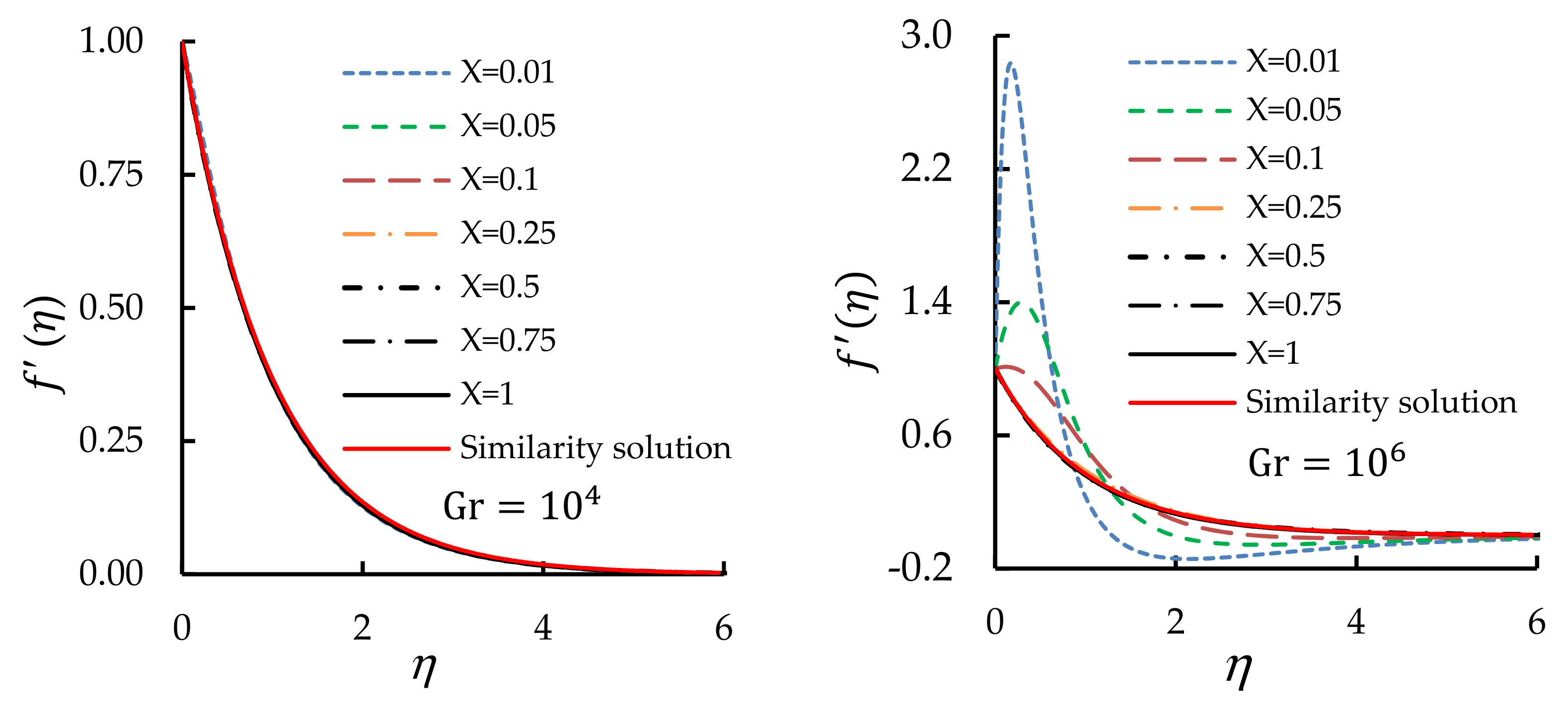
- The similarity analysis could not approximate the flow characteristics near the extrusion slit at low values of Reynolds numbers.
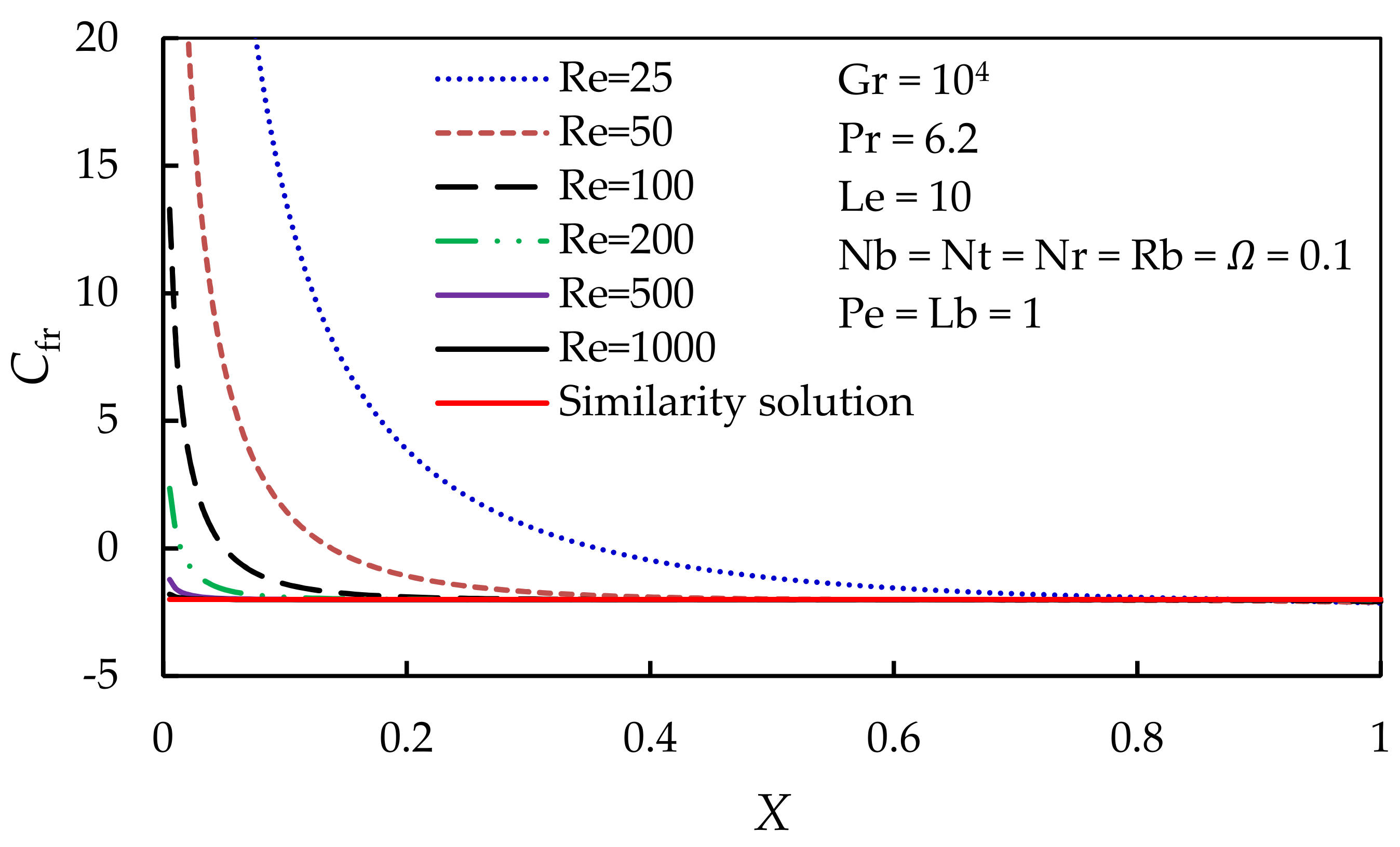
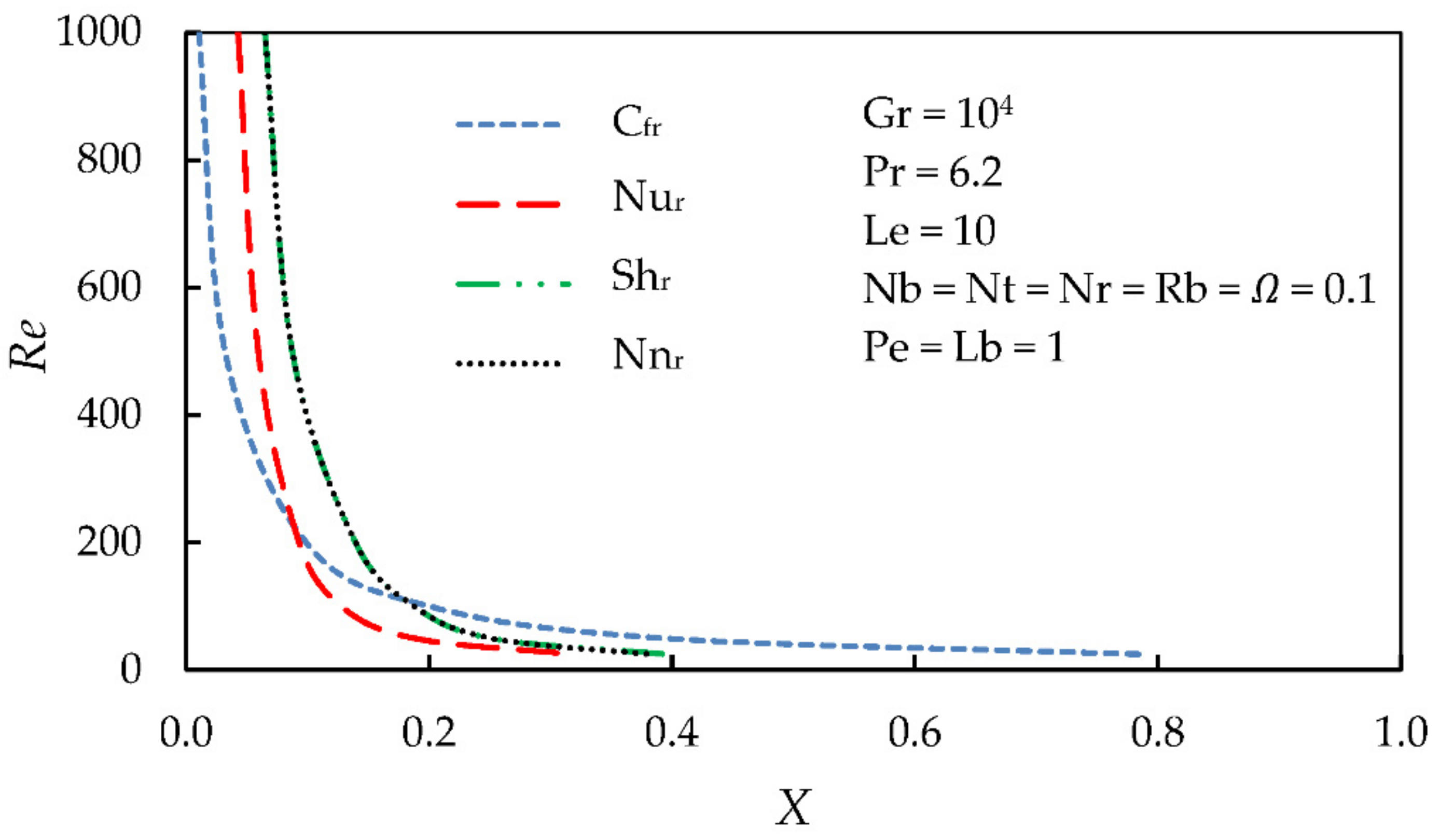
- Having a mismatch less than 5% between the CFD and the similarity analysis at a position of 6.5% of the way along the sheet, the critical Reynolds number above which the similarity analysis matched the computational fluid dynamics solution was more than 1000 for Gr = 104, Pr = 6.2, Le = 10, Nb = Nt = Nr = Rb = Ω = 0.1, and Pe = Lb = 1.
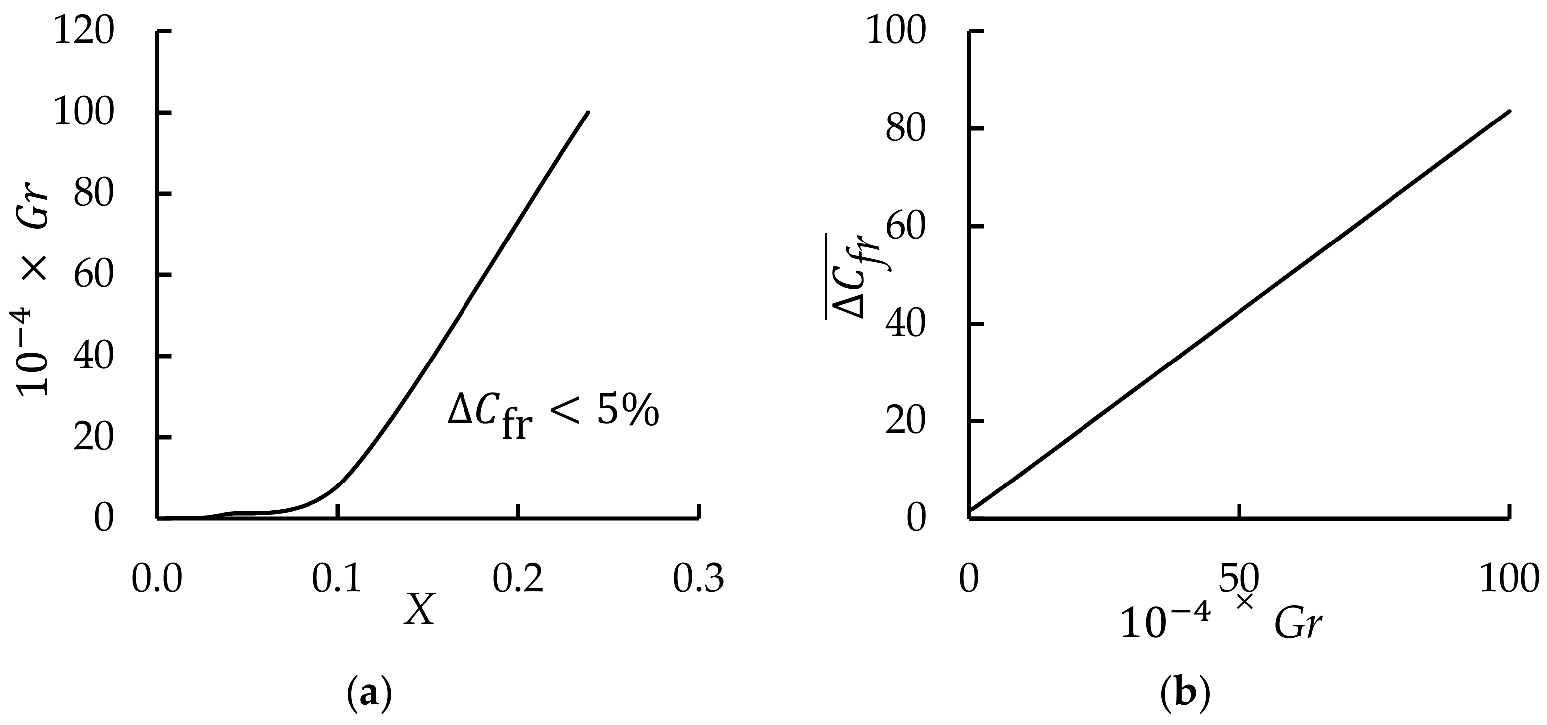
- An increase in the Grashof number, Gr, increased the length of the region in which the flow was undeveloped, leading to a decrease in the reliability of the similarity analysis. It was found that the similarity analysis was within 5% of the computational fluid dynamics solution at a position of 10% of the way along the sheet and beyond this for Gr < 8 × 10⁴, Re = 400, Pr = 6.2, Le = 10, Nb = Nt = Nr = Rb = Ω = 0.1, and Pe = Lb = 1.
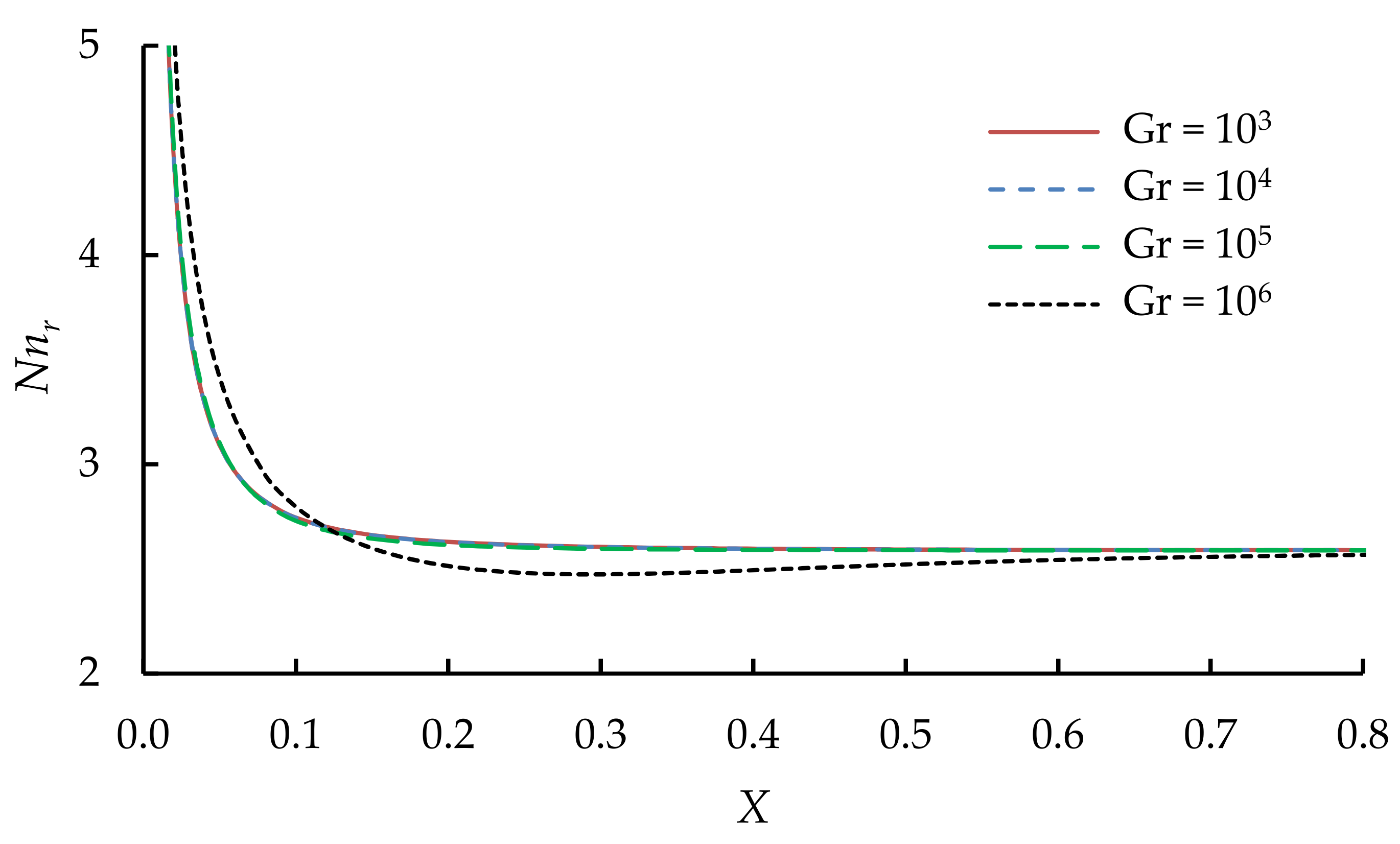
- Increasing the Grashof number from 103 to 105 did not affect the length of the region in which there was no fully developed boundary layer for the density of the microorganisms. However, this region diminished strongly as the Grashof number increased from 105 to 106.
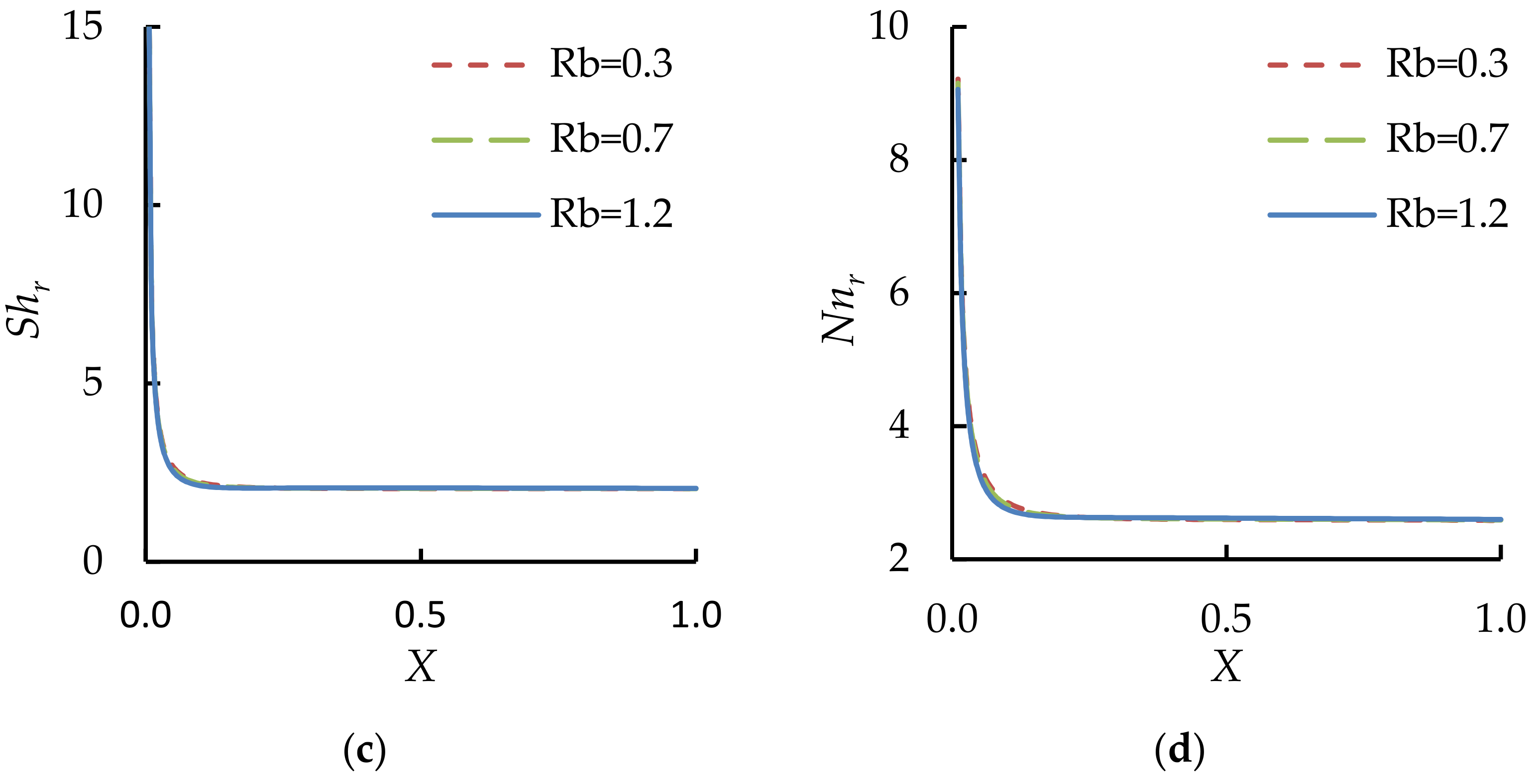
- Increasing the bioconvection Rayleigh number, Rb, caused the reduced skin friction coefficient, Cfr, to decrease, but had a weaker effect on the reduced Nusselt number, Nur, the reduced Sherwood number, Shr, and the reduced concentration of microorganisms, Nnr.
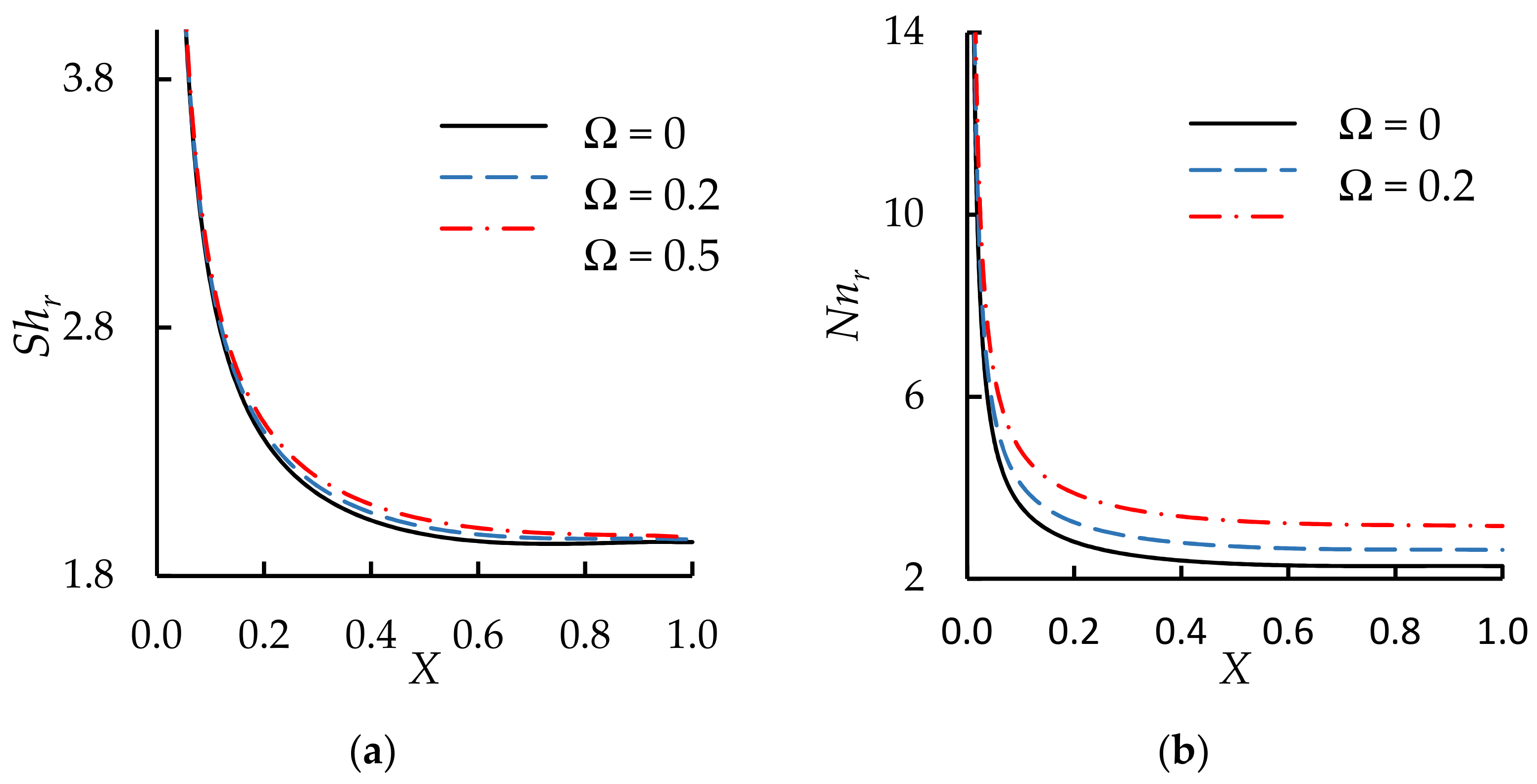
- Increasing the difference in the density of the microorganisms from the surface to the far-field, , led to an increase in the reduced Nusselt number, Nur.
Author Contributions
Funding
Institutional Review Board Statement
Informed Consent Statement
Data Availability Statement
Acknowledgments
Conflicts of Interest
References
- Vajravelu, K.; Prasad, K.; Lee, J.; Lee, C.; Pop, I.; Van Gorder, R.A. Convective heat transfer in the flow of viscous Ag–water and Cu–water nanofluids over a stretching surface. Int. J. Therm. Sci. 2011, 50, 843–851. [Google Scholar] [CrossRef]
- Hakeem, A.A.; Kalaivanan, R.; Ganesh, N.V.; Ganga, B. Effect of partial slip on hydromagnetic flow over a porous stretching sheet with non-uniform heat source/sink, thermal radiation and wall mass transfer. Ain Shams Eng. J. 2014, 5, 913–922. [Google Scholar] [CrossRef] [Green Version]
- Nandy, S.K.; Pop, I. Effects of magnetic field and thermal radiation on stagnation flow and heat transfer of nanofluid over a shrinking surface. Int. Commun. Heat Mass Transf. 2014, 53, 50–55. [Google Scholar] [CrossRef]
- Noghrehabadi, A.; Izadpanahi, E.; Ghalambaz, M. Analyze of fluid flow and heat transfer of nanofluids over a stretching sheet near the extrusion slit. Comput. Fluids 2014, 100, 227–236. [Google Scholar] [CrossRef]
- Ferdows, M.; Uddin, M.J.; Afify, A. Scaling group transformation for MHD boundary layer free convective heat and mass transfer flow past a convectively heated nonlinear radiating stretching sheet. Int. J. Heat Mass Transf. 2013, 56, 181–187. [Google Scholar] [CrossRef]
- Sahoo, B.; Do, Y. Effects of slip on sheet-driven flow and heat transfer of a third grade fluid past a stretching sheet. Int. Commun. Heat Mass Transf. 2010, 37, 1064–1071. [Google Scholar] [CrossRef]
- Mukhopadhyay, S. MHD boundary layer flow and heat transfer over an exponentially stretching sheet embedded in a thermally stratified medium. Alex. Eng. J. 2013, 52, 259–265. [Google Scholar] [CrossRef] [Green Version]
- Ibrahim, W.; Shankar, B. MHD boundary layer flow and heat transfer of a nanofluid past a permeable stretching sheet with velocity, thermal and solutal slip boundary conditions. Comput. Fluids 2013, 75, 1–10. [Google Scholar] [CrossRef]
- Alsaedi, A.; Awais, M.; Hayat, T. Effects of heat generation/absorption on stagnation point flow of nanofluid over a surface with convective boundary conditions. Commun. Nonlinear Sci. Numer. Simul. 2012, 17, 4210–4223. [Google Scholar] [CrossRef]
- Madhukesh, J.; Kumar, R.N.; Gowda, R.P.; Prasannakumara, B.; Ramesh, G.; Khan, M.I.; Khan, S.U.; Chu, Y.-M. Numerical simulation of AA7072-AA7075/water-based hybrid nanofluid flow over a curved stretching sheet with Newtonian heating: A non-Fourier heat flux model approach. J. Mol. Liq. 2021, 335, 116103. [Google Scholar] [CrossRef]
- Aslani, K.-E.; Mahabaleshwar, U.S.; Singh, J.; Sarris, I.E. Combined Effect of Radiation and Inclined MHD Flow of a Micropolar Fluid Over a Porous Stretching/Shrinking Sheet with Mass Transpiration. Int. J. Appl. Comput. Math. 2021, 7, 1–21. [Google Scholar] [CrossRef]
- Murtaza, M.; Tzirtzilakis, E.E.; Ferdows, M. Stability and convergence analysis of a biomagnetic fluid flow over a stretching sheet in the presence of a magnetic field. Symmetry 2020, 12, 253. [Google Scholar] [CrossRef] [Green Version]
- Rehman, A.; Salleh, Z.; Gul, T.; Zaheer, Z. The impact of viscous dissipation on the thin film unsteady flow of GO-EG/GO-W nanofluids. Mathematics 2019, 7, 653. [Google Scholar] [CrossRef] [Green Version]
- Anuar, N.S.; Bachok, N.; Pop, I. Cu-Al2O3/water hybrid nanofluid stagnation point flow past MHD stretching/shrinking sheet in presence of homogeneous-heterogeneous and convective boundary conditions. Mathematics 2020, 8, 1237. [Google Scholar] [CrossRef]
- Ghalambaz, M.; Groşan, T.; Pop, I. Mixed convection boundary layer flow and heat transfer over a vertical plate embedded in a porous medium filled with a suspension of nano-encapsulated phase change materials. J. Mol. Liq. 2019, 293, 111432. [Google Scholar] [CrossRef]
- Sarada, K.; Gowda, R.J.P.; Sarris, I.E.; Kumar, R.N.; Prasannakumara, B.C. Effect of Magnetohydrodynamics on Heat Transfer Behaviour of a Non-Newtonian Fluid Flow over a Stretching Sheet under Local Thermal Non-Equilibrium Condition. Fluids 2021, 6, 264. [Google Scholar] [CrossRef]
- Choi, S.U.; Eastman, J.A. Enhancing Thermal Conductivity of Fluids with Nanoparticles; Argonne National Laboratory: Lemont, IL, USA, 1995. [Google Scholar]
- Ramesh, G.; Madhukesh, J.; Prasannakumara, B.; Roopa, G. Significance of aluminium alloys particle flow through a parallel plates with activation energy and chemical reaction. J. Therm. Anal. Calorim. 2021, 1–11. [Google Scholar] [CrossRef]
- Kumar, A.; Subudhi, S. Preparation, characterization and heat transfer analysis of nanofluids used for engine cooling. Appl. Therm. Eng. 2019, 160, 114092. [Google Scholar] [CrossRef]
- Esfahani, M.R.; Languri, E.M. Exergy analysis of a shell-and-tube heat exchanger using graphene oxide nanofluids. Exp. Therm. Fluid Sci. 2017, 83, 100–106. [Google Scholar] [CrossRef]
- Oliveira, G.A.; Contreras, E.M.C.; Bandarra Filho, E.P. Experimental study on the heat transfer of MWCNT/water nanofluid flowing in a car radiator. Appl. Therm. Eng. 2017, 111, 1450–1456. [Google Scholar] [CrossRef]
- Siricharoenpanich, A.; Wiriyasart, S.; Srichat, A.; Naphon, P. Thermal cooling system with Ag/Fe3O4 nanofluids mixture as coolant for electronic devices cooling. Case Stud. Therm. Eng. 2020, 20, 100641. [Google Scholar] [CrossRef]
- Wang, X.; Xu, X.; Choi, S.U. Thermal conductivity of nanoparticle-fluid mixture. J. Thermophys. Heat Transf. 1999, 13, 474–480. [Google Scholar] [CrossRef]
- Das, S.K.; Putra, N.; Roetzel, W. Pool boiling of nano-fluids on horizontal narrow tubes. Int. J. Multiph. Flow 2003, 29, 1237–1247. [Google Scholar] [CrossRef]
- Xie, H.; Wang, J.; Xi, T.; Liu, Y.; Ai, F.; Wu, Q. Thermal conductivity enhancement of suspensions containing nanosized alumina particles. J. Appl. Phys. 2002, 91, 4568–4572. [Google Scholar] [CrossRef]
- Das, S.K.; Putra, N.; Thiesen, P.; Roetzel, W. Temperature dependence of thermal conductivity enhancement for nanofluids. J. Heat Transf. 2003, 125, 567–574. [Google Scholar] [CrossRef]
- Drew, D.A.; Passman, S.L. Theory of Multicomponent Fluids; Springer Science & Business Media: Berlin/Heidelberg, Germany, 2006. [Google Scholar]
- Yang, L.; Ji, W.; Huang, J.-N.; Xu, G. An updated review on the influential parameters on thermal conductivity of nano-fluids. J. Mol. Liq. 2019, 296, 111780. [Google Scholar] [CrossRef]
- Noorzadeh, S.; Moghanlou, F.S.; Vajdi, M.; Ataei, M. Thermal conductivity, viscosity and heat transfer process in nanofluids: A critical review. J. Compos. Compd. 2020, 2, 175–192. [Google Scholar]
- Sun, C.; Fard, B.E.; Karimipour, A.; Abdollahi, A.; Bach, Q.-V. Producing ZrO2/LP107160 NF and presenting a correlation for prediction of thermal conductivity via GMDH method: An empirical and numerical investigation. Phys. E Low Dimens. Syst. Nanostruct. 2021, 127, 114511. [Google Scholar] [CrossRef]
- Das, P.K. A review based on the effect and mechanism of thermal conductivity of normal nanofluids and hybrid nanofluids. J. Mol. Liq. 2017, 240, 420–446. [Google Scholar] [CrossRef]
- Moldoveanu, G.M.; Huminic, G.; Minea, A.A.; Huminic, A. Experimental study on thermal conductivity of stabilized Al2O3 and SiO2 nanofluids and their hybrid. Int. J. Heat Mass Transf. 2018, 127, 450–457. [Google Scholar] [CrossRef]
- Bees, M.A. Advances in bioconvection. Annu. Rev. Fluid Mech. 2020, 52, 449–476. [Google Scholar] [CrossRef]
- Aslani, Κ.-E.; Sarris, I.E. Effect of micromagnetorotation on magnetohydrodynamic Poiseuille micropolar flow: Analytical solutions and stability analysis. J. Fluid Mech. 2021, 920, A25. [Google Scholar] [CrossRef]
- Jain, S.; Choudhary, R. Bioconvection Flow and Heat Transfer over a Stretching Sheet in the Presence of Both Gyrotactic Microorganism and Nanoparticle Under Convective Boundary Conditions and Induced Magnetic Field. In Engineering Vibration, Communication and Information Processing; Springer: Berlin/Heidelberg, Germany, 2019; pp. 651–668. [Google Scholar]
- Yusuf, T.A.; Mabood, F.; Prasannakumara, B.; Sarris, I.E. Magneto-Bioconvection Flow of Williamson Nanofluid over an Inclined Plate with Gyrotactic Microorganisms and Entropy Generation. Fluids 2021, 6, 109. [Google Scholar] [CrossRef]
- Sokolov, A.; Goldstein, R.E.; Feldchtein, F.I.; Aranson, I.S. Enhanced mixing and spatial instability in concentrated bacterial suspensions. Phys. Rev. E 2009, 80, 031903. [Google Scholar] [CrossRef] [Green Version]
- Kuznetsov, A. The onset of nanofluid bioconvection in a suspension containing both nanoparticles and gyrotactic microorganisms. Int. Commun. Heat Mass Transf. 2010, 37, 1421–1425. [Google Scholar] [CrossRef]
- Khan, W.; Makinde, O.; Khan, Z. MHD boundary layer flow of a nanofluid containing gyrotactic microorganisms past a vertical plate with Navier slip. Int. J. Heat Mass Transf. 2014, 74, 285–291. [Google Scholar] [CrossRef]
- Mehryan, S.M.; Moradi Kashkooli, F.; Soltani, M.; Raahemifar, K. Fluid flow and heat transfer analysis of a nanofluid containing motile gyrotactic micro-organisms passing a nonlinear stretching vertical sheet in the presence of a non-uniform magnetic field; numerical approach. PLoS ONE 2016, 11, e0157598. [Google Scholar] [CrossRef]
- Jawad, M.; Shehzad, K.; Safdar, R.; Hussain, S. Novel computational study on MHD flow of nanofluid flow with gyrotactic microorganism due to porous stretching sheet. Punjab Univ. J. Math. 2020, 52, 43–60. [Google Scholar]
- Shahid, A.; Huang, H.; Bhatti, M.M.; Zhang, L.; Ellahi, R. Numerical investigation on the swimming of gyrotactic microorganisms in nanofluids through porous medium over a stretched surface. Mathematics 2020, 8, 380. [Google Scholar] [CrossRef] [Green Version]
- Sulaiman, M.; Ali, A.; Islam, S. Heat and mass transfer in three-dimensional flow of an Oldroyd-B nanofluid with gyrotactic micro-organisms. Math. Probl. Eng. 2018, 6790420. [Google Scholar] [CrossRef] [Green Version]
- Song, Y.-Q.; Hamid, A.; Khan, M.I.; Gowda, R.P.; Kumar, R.N.; Prasannakumara, B.; Khan, S.U.; Khan, M.I.; Malik, M. Solar energy aspects of gyrotactic mixed bioconvection flow of nanofluid past a vertical thin moving needle influenced by variable Prandtl number. Chaos Solitons Fractals 2021, 151, 111244. [Google Scholar] [CrossRef]


| Grid Size | Nnr | Error % | Shr | Error % | Nur | Error % | Cfr | Error % |
|---|---|---|---|---|---|---|---|---|
| 60 × 60 | 2.3153 | 13.43 | 1.7885 | 15.28 | 1.6153 | 71.20 | −1.781 | 11.72 |
| 90 × 90 | 2.6747 | 0.40 | 2.1110 | 0.56 | 0.9435 | 3.37 | −2.018 | 1.67 |
| 135 × 135 | 2.6639 | 0.02 | 2.0992 | 0.11 | 0.9764 | 0.78 | −1.985 | 0.52 |
| 200 × 200 | 2.6644 | - | 2.1015 | - | 0.9841 | - | −1.995 | - |
Publisher’s Note: MDPI stays neutral with regard to jurisdictional claims in published maps and institutional affiliations. |
© 2021 by the authors. Licensee MDPI, Basel, Switzerland. This article is an open access article distributed under the terms and conditions of the Creative Commons Attribution (CC BY) license (https://creativecommons.org/licenses/by/4.0/).
Share and Cite
Hosseini, Z.S.; Abidi, A.; Mohammadi, S.; Mehryan, S.A.M.; Hulme, C. A Fully Resolved Computational Fluid Dynamics Study of the Boundary Layer Flow of an Aqueous Nanoliquid Comprising Gyrotactic Microorganisms over a Stretching Sheet: The Validity of Conventional Similarity Models. Mathematics 2021, 9, 2655. https://doi.org/10.3390/math9212655
Hosseini ZS, Abidi A, Mohammadi S, Mehryan SAM, Hulme C. A Fully Resolved Computational Fluid Dynamics Study of the Boundary Layer Flow of an Aqueous Nanoliquid Comprising Gyrotactic Microorganisms over a Stretching Sheet: The Validity of Conventional Similarity Models. Mathematics. 2021; 9(21):2655. https://doi.org/10.3390/math9212655
Chicago/Turabian StyleHosseini, Zahra Shah, Awatef Abidi, Sajad Mohammadi, Seyed Abdollah Mansouri Mehryan, and Christopher Hulme. 2021. "A Fully Resolved Computational Fluid Dynamics Study of the Boundary Layer Flow of an Aqueous Nanoliquid Comprising Gyrotactic Microorganisms over a Stretching Sheet: The Validity of Conventional Similarity Models" Mathematics 9, no. 21: 2655. https://doi.org/10.3390/math9212655
APA StyleHosseini, Z. S., Abidi, A., Mohammadi, S., Mehryan, S. A. M., & Hulme, C. (2021). A Fully Resolved Computational Fluid Dynamics Study of the Boundary Layer Flow of an Aqueous Nanoliquid Comprising Gyrotactic Microorganisms over a Stretching Sheet: The Validity of Conventional Similarity Models. Mathematics, 9(21), 2655. https://doi.org/10.3390/math9212655