A Chemical Analysis of Hybrid Economic Systems—Tokens and Money

Abstract

With the influence of digital technology in our daily lives continuously growing, we investigate methods with the purpose of assessing the stability, sustainability, and design of systems of token economies that include tokens and conventional currencies. Based on a chemical approach, we model markets with a minimum number of variables and compare the transaction rates, stability, and token design properties at different levels of tokenisation. The kinetic study reveals that in certain conditions, if the price of a product contains both conventional money and tokens, one can treat this combination as one composite currency. The dynamic behaviour of the analysed systems is proven to be dynamically stable for the chosen models. Moreover, by applying the supply and demand law to recalculate the prices of products, the necessity of previous knowledge of certain token attributes—token divisibility and token–money exchange rates—emerges. The chemical framework, along with the analytic methods that we propose, is flexible enough to be adjusted to a variety of conditions and offer valuable information about economic systems.

1. Introduction

According to the United Nations, “digital technologies have advanced more rapidly than any innovation in our history—reaching around 50 per cent of the developing world’s population in only two decades and transforming societies [1]”. Digital technologies (DTs) are also on the international list of priorities for a better recovery from the ongoing pandemic [2].

DTs have permeated our daily lives and will continue to do so [3]. The business world is essentially driven by digital transformation [4,5]. At the same time, large-scale DT applications are being developed, for example, with the objective of embedding digitalisation in urban planning [6], with projects underway in major cities in Europe and beyond [7,8]. In this context, subjects such as the trust of the public, security, and the long-term sustainability of DTs are imperative to study and understand [9,10].

Blockchain technology is an example of a DT that has the potential to reshape and redesign all social activities as pervasively as the invention of the internet [11]. As a mode of decentralisation, among other things, blockchain technology and cryptocurrency are basic technologies that businesses can make use of in the digital transformation process [12,13]. The notions of cryptocurrency and tokens are tightly linked. Cryptocurrencies are digital tokens that exist within a specific cryptocurrency system [14]. Native tokens are used to incentivise participants to run a network in the absence of a central authority [14]. Furthermore, tokens provide the means for utilising certain blockchain services [15] or can be seen as a privately used type of currency [16].

Blockchain technology can be used on smaller scales, such as in local communities, allowing the creation of local cryptocurrencies and specifically tailored economic policies. Coupled with the concept of behavioural incentives in the shape of tokens [17,18], cryptocurrencies and token economies can significantly empower local communities [19]. In practice, there are more and more initiatives and startups that are incorporating incentive tokens into their business models in a variety of ways [20,21,22,23,24].

There have been recent studies on the consequences of certain types of tokens being incorporated into business models and networks, e.g., Initial Coin Offerings (ICOs) in startups [25,26] and on multi-sided platforms, such as Amazon, Uber, and Airbnb [27], or ERC20-compatible tokens in token networks [28].

However, there is no study, to our knowledge, that has proposed a model based on basic economic principles aimed in order to describe the transitions and stability of small- and medium-scale businesses that start to introduce tokens to incentivise the sale of certain products (e.g., imperfect, recycled, and second-hand products or niche and luxury goods). As blockchain technology becomes even more widely accessible, in addition to benefits such as the autonomy of the system and the possibilities of trading with tokens, enterprises rooted in local communities might want to introduce tokens in an already fully developed business. This phenomenon would give rise to a multitude of hybrid economic systems involving both conventional currencies (money) and tokens.

This paper proposes a new, chemical-inspired model of trading with multiple currencies, where the act of trading is modelled as a chemical reaction between molecules (the product, the tokens). It also proposes investigative methods with the main aim of assessing stability and sustainability and helping with the design of a token economy. A token economy here refers to a system that includes tokens in addition to conventional currencies. We offer analytical tools for comparing conventional market sales and transactions to several degrees of token involvement in similar systems, thus highlighting the benefits and downsides of tokenisation.

The approach of this analysis comes from the perspective of econophysics (or rather econochemistry). Econophysics [29] aims to understand economic systems from the point of view of statistical physics, complex systems, and network science, as well as to address current challenges in economic systems, such as extreme events, cascading effects, and financial instabilities [30]. While physics and economy/sociology have been intertwined for decades [31], there is constant negotiation and compromise in modelling complex systems displaying emergent behaviour [32] with deterministic physical/chemical models. In this paper, we focus on the most important advantage of this approach: By restricting the model to the minimum number of variables needed, the physical model facilitates an analytical treatment and better understanding of some aspects of the economic system for the purpose of prediction [33].

There are already many analogies between chemical processes and complex economic systems—for example, the connection of chemical reactors [34] or coupled flare attractors [35] with economics and finance. The present chemical model draws a direct equivalence between ideal gases that chemically interact and products, money, and market transactions, thus giving rise to chemical reaction equations that can exhibit oscillatory or chaotic dynamics [36,37], making them a perfect tool for stability analysis [38,39]. Indeed, the chemical reaction equations, based on a model of atomic-level interactions, allow for the analysis of macroscopic variables, such as the behaviour of the concentration of a solution over time and the stability of a system.

In this paper, we present three methods of analysis that provide important information about economic systems. Both of the first two methods target the changes in reaction rates and the variations in the concentrations of molecules. The third method is the implementation of the demand and supply law, and it is complementary to the first two. Three systems are constructed, modelled as chemical reaction mechanisms, and analysed from different perspectives. The models themselves are general enough to illustrate fundamental differences in the token economy design and flexible enough to be extended and tailored for more specific applications.

The justification for and detailed overview of the equivalence between chemical reactions and market transactions is described in Section 2.1, followed by the presentation of the chemical model in Section 2.2.

The first of the analytical methods is a kinetic study (described in Section 2.3). Kinetic analysis relies on data about previous quantities being sold. It can be applied for planning changes in preexisting systems, where it provides an overview of the time dependence of the quantities involved. In this study, we show how the introduction of tokens alongside conventional money can be treated as one composite currency under certain circumstances, and that the result will have the same time profile as that of conventional currency.

The second method is stability analysis, which can be applied to the design of new and more complex systems (described in Section 2.4), and the outcome provides information on the stability of the system as a whole rather than the behaviour of the components of the chemical reactions over time. It is a purely theoretical model, and hence, it does not require any previous data. It reveals the behaviour of the designed system to be stable, oscillatory, or unstable. Desirable behaviour for a new economic system can either be stable or oscillatory around critical points (steady states). Any sign of instability can lead to potentially chaotic behaviour and to unpredictable outcomes. In our particular cases, the behaviour in the vicinity of the critical states is mainly stable, with only one case of unstable equilibrium.

The third method proposed in this study (Section 2.5) is an economic approach for open markets and, specifically, the recalculation of prices according to the law of demand and supply. To be consistent, we discuss the steps and the outcomes referring to the chemical models introduced previously. However, at its core, this method has little to do with the chemical assumptions made in the first two techniques. Consequently, this third method can supplement either of the previous ones. The novelty that this method provides is to bring to light the ways that the architect of an economic system can regard the introduced tokens: as one indivisible unit, as a second type of currency with an exchange rate between the tokens and the conventional currency, or as a divisible standalone currency.

The results of this study are presented in Section 3, we provide some discussion in Section 4, and our conclusions are presented in Section 5. The link to the git repository, including the scripts with which the figures were generated, can be found in the Supplementary Materials.

2. Materials and Methods

2.1. The Connection between Chemical Reactions and Market Transactions

At the micro level, a market is characterised by the exchange of services or goods, usually for money. In a sense, an exchange happens when a buyer and a seller, endowed with the right elements (goods and amounts of money), meet and interact, creating a transaction. A chemical reaction is also an interaction between different molecules, resulting in the creation of different molecules. We can thus draw a parallel between the market transaction and the chemical transaction, where goods and money are molecules that react together, turning into a new element that represents a successful transaction.

If we imagine two ideal gases, the “product gas” and the “money gas”, interacting in a volume that represents the market, transactions are formed through collisions between product and money molecules. Other chemical parameters find easy analogies with the market as well: The reaction rate factors could be related to characteristics of individual transactions—for example, the activation energy ($E_A$) might be proportional to the demand for this particular product and the steric factor ($\rho$) to the individual customer decision to buy.

The advantage of this approach is the ease with which new kinds of money can be added to the market by simply modifying the equation specifying the reactions. However, this approach abstracts away the individuality of the buyers and sellers, modelling only the overall availability of money and goods, and should be used with caution in cases where this is important—for example, in cases where oligopolies can influence the market.

The chemical model captures small-scale market transactions (individuals exchanging products for money) at an atomic level while allowing for large-scale aspects of the systems to be analysed: price adjustments, the stability of the entire system, token attributes, etc., which are equivalent to measurable quantities, such as solution concentration. In this sense, the chemical model is an accurate enough abstraction to allow for the analysis of certain small-scale aspects of the market (the introduction of tokens in transactions) while, at the same time, being a suitable enough model to capture some of the emerging larger-scale system characteristics.

To be more specific, we model reactions between molecules of the following different classes. The product class corresponds to actual products of different kinds, while molecules of the money class correspond to circulating money, and thus represent overall demand for the product. Molecules of the transaction class represent the materialisation of a transaction that happens when a product element meets a money element.

At a microscopic level, reactions in a gas happen when different atoms/molecules collide. By modelling market transactions as collisions, we abstract from the details of how buyers meet customers in the market, assuming that these events will happen in a uniformly random way. Thus, the model applies to markets that reach closure quickly and where prices do not change or change too slowly to intervene in the course of a single reaction. The price of all products is dictated by the coefficients of the different types of products taking part in the reactions. Assuming that molecules are neither added nor removed, after the reaction starts, the chemical reaction will stop when the reagents are exhausted. Thus, given the initial state of the system, it is always possible to calculate a final state. In reality, one can model more complex markets with changing prices and types of products as a sequence of chemical reaction mechanisms. We are describing here the model for one step in a chronology of events because the chemical reaction mechanisms cannot be defined for variable coefficients.

In the following, we develop the formulas for reactions under the ideal gas law assumption and in the collision theory framework. We indicate the reaction rate as $r_{rate}=\rho Z_{AB}f$, where $\rho$ is the steric factor (that accounts for the orientation of the collisions), $Z_{AB}$ is the collision density (a function of the reactant concentrations), and f is the fraction of molecules with enough energy to overcome the activation barrier (a function of the activation energy of the reaction $E_A$).

2.2. Chemical Model

In the general description of the chemical model, we present three reaction mechanisms, with one of them describing a set of transactions using only conventional money (referred to as RM1 where RM stands for reaction mechanism throughout the paper). The second and third reaction mechanisms, RM2 and RM2s, involve an additional type of currency, namely tokens.

The molecules in the reaction include the product (Z), which can, in turn, transform into two different product molecules ($X,Y$)—for example, because of different qualities or desirability. These latter molecules are exchanged on the market for one type of currency (A) in the first reaction mechanism (RM1), and the exchange results in a transaction (T). Here, $\alpha$ and $\beta$ represent fractions of the product subgroups (being modelled as reaction coefficients), while c and d are the coefficients of the currency type (always positive integers).

Table 1. Overview of the chemical molecules and examples of their possible interpretations.

Chem. Elem.	Possible Interpretations
Z	Total amount of produce coming from a single supplier (e.g., vegetables), Total amount of produced goods, e.g., clothing, furniture
X	Products not usually desired by most customers: imperfect products, e.g., tomatoes, used/not new goods, e.g., out-of-fashion clothing, second-hand furniture, recycled paper goods, e.g., notebooks
Y	Niche or impactful products: organically sourced produce, traditional products (e.g., clothing) supporting local businesses, environmentally friendly building materials, renewable energy sources, low-power electronics
A	Conventional currency
B	Token(s) received for actions such as: consuming imperfect fruits and vegetables, buying second-hand goods, donating food and goods to the community, taking part in clean-up projects in nature, volunteering activities that benefit the community, minimising one’s CO${}_2$ footprint
T	Market transactions

summarises the chemical species and a few examples of what they might represent.

Equations (1)–(4) represent RM1:

$$Z\stackrel{k}{\to }\alpha X+\beta Y$$

(1)

$$X+cA\stackrel{k_1}{\to }T$$

(2)

$$Y+dA\stackrel{k_2}{\to }T$$

(3)

with $k,k_1$, and $k_2$ being reaction rate constants. Multiplying Equation (2) by $\alpha$, Equation (3) by $\beta$, and summing up all the equations according to the law of conservation of mass, the net reaction of RM1 is:

$$Z+(\alpha c+\beta d)A\to (\alpha +\beta )T$$

(4)

For RM2, we start with the same premise (Equation (1)), but we introduce tokens (B). The main difference is that if in RM1, the two types of products are sold independently, RM2 binds the selling of product Y to X by introducing tokens (Equations (6) and (7)). These are created in the process of buying X in order to incentivise either the selling of these products or to increase the selling price for X (assuming $f>c$). The created token B takes part as payment in the transaction involving product Y. If $\alpha <\beta$, the tokens will run out before all of product Y is sold. Therefore, we allow the option of purchasing Y in the same way as in RM1 as well (Equation (8)).

$$Z\stackrel{k}{\to }\alpha X+\beta Y$$

(5)

$$X+fA\stackrel{k_3}{\to }B+T$$

(6)

$$Y+B+gA\stackrel{k_4}{\to }T$$

(7)

$$Y+dA\stackrel{k_5}{\to }T$$

(8)

Multiplying Equations (6) and (7) by $\alpha$ and Equation (8) by ($\beta -\alpha$) so that Y adds up to $\beta$, the net reaction of RM2 becomes:

$$Z+\left[\alpha \right(f+g-d)+\beta d]A\to (\alpha +\beta )T$$

(9)

A more restrictive chemical mechanism is considered as well (RM2s), in which the second channel for selling product Y is removed, forcing Y to be sold only through a combination of conventional currency and tokens. RM2s is described exclusively by Equations (5)–(7).

While Equation (1) is not necessary for the reaction mechanism, it helps to conceptualise the model in terms of tokenising and intertwining the prices for two sub-types of products. In addition, Equation (1)represents a common product base for all three systems (RM1, RM2, and RM2s), keeping the same fractions of products X and Y in the reactions for comparison.

By comparing Equations (4) and (9), one can see how the total number of transactions in both systems is the same. Moreover, if $f+g-d=c$, the amount of money (A) involved in the chemical mechanisms is the same in RM1 and RM2.

The way in which the chemical reaction mechanisms are constructed allows for the modelling of special cases, such as:

• $\alpha =\beta$: X and Y enter the reactions/market in exactly the same quantity.
• $f=c$ and $g=d$: The presence of the tokens in the reactions is superfluous.
• $g=0$: In the RM2s context, this means that product Y can be bought with tokens only. This strategy can be used to reward loyal customers instead of introducing vouchers.
• $f>c$ and $g<d$: Tokens are fully integrated and play an active role in the pricing of the products.
• $\alpha >\beta$: By starting with more of product X than Y, one may end up with a surplus of tokens at the end of the reactions that will have to be transferred and accounted for in the subsequent reaction mechanism.
• $\alpha <\beta$: One might run out of tokens in this step of the sequence of reaction mechanisms simply because selling product X will not generate enough tokens to buy all of the Y products. This is not an issue in RM2, but might become one in RM2s, where selling Y is restricted to token involvement.
• One can also imagine supplementing the reaction mechanisms with a way to buy X only with tokens at later stages.

2.3. Kinetic Study

The kinetic study of a chemical reaction or of a chemical mechanism is the study of its reaction rates. It establishes the variation over time of the concentrations of molecules based on measurements and observational data. It offers a time profile for the components taking part in transactions in a given time interval. A kinetic study offers important information not just about the behaviour of new components, such as tokens, but also on how their presence influences the speed or efficiency at which products are being sold.

In this section, we make the assumption that chemical reactions are not elementary reactions (meaning that there is no direct correspondence between the order of reactions and their stoichiometry/coefficient). While treating their analysis similarly, one can imagine a scenario in which the product (X or Y) is in unlimited supply. Changing the quantity (due to the fact that the described transactions happen in a market, a closed space, we take the liberty of using “concentration” and “quantity” interchangeably throughout the paper) of the product in this case has no effect on the rate of the reaction. However, the more money there is available, the faster the transactions will happen.

If we use square brackets for concentration (e.g., $\left[A\right]$ is the concentration of molecule A) and $r_x$ for the reaction rate (e.g., $r_2$ is the reaction rate of Equation (2)), we can draw some simple conclusions from the model. First, if the relationship between money and the reaction rate is linear, the reaction rate will become first order with respect to $\left[A\right]$ and zero order with respect to $\left[X\right]$ or $\left[Y\right]$: $r_2=k{\left[X\right]}^0{\left[A\right]}^1$ and $r_3=k{\left[Y\right]}^0{\left[A\right]}^1$, where the type of notation $r_2$ refers to the reaction rate of Equation (2). If, on the other hand, the demand for the product is unlimited and the product is in short supply, only the product quantity will have an effect on the reaction rate, and hence, the rate will become first order with respect to $\left[X\right]$ or $\left[Y\right]$ and zero order with respect to $\left[A\right]$: $r_2=k{\left[X\right]}^1{\left[A\right]}^0$ and $r_3=k{\left[Y\right]}^1{\left[A\right]}^0$. All of the reaction rates (including those for Equations (6)–(8)) can be found in

Table 2. The expressions for the reaction rates in RM1 and RM2s for the two cases in which the quantity of money is much larger than the quantity of products and vice versa.

Cases	Reaction Rates in RM1—Equations (2) and (3)	Reaction Rates in RM2s—Equations (6)–(8)
	$r_2=k_1{\left[X\right]}^1{\left[A\right]}^0$	$r_6=k_3{\left[X\right]}^1{\left[A\right]}^0$
$\left[A\right]\gg \left[Z\right]$	$r_3=k_2{\left[Y\right]}^1{\left[A\right]}^0$	$r_7=k_4{\left[Y\right]}^1{\left[C\right]}^0$
		$r_8=k_5{\left[Y\right]}^1{\left[A\right]}^0$
$\left[Z\right]\gg \left[A\right]$	$r_2=k_1{\left[X\right]}^0{\left[A\right]}^1$	$r_6=k_3{\left[X\right]}^0{\left[A\right]}^1$
	$r_3=k_2{\left[Y\right]}^0{\left[A\right]}^1$	$r_7=k_4{\left[Y\right]}^0{\left[C\right]}^1$

. Reaction rates can be of the second order with respect to the concentrations of certain components too, meaning that doubling the concentration of a component will quadruple the reaction rate; while this situation is quite common, we do not discuss it in this paper.

Intuitively, the price of a product can be adjusted by changing the coefficients c and d (the higher their value, the higher the price). In order for the reaction mechanism to be stoichiometrically balanced, we need the coefficients to be constant throughout the reaction, meaning that the price of the product has to remain constant. This scenario happens only at market equilibrium, ensuring as well that there is no surplus and no storage of goods. This is the reason for why we cannot supplement the rate equations with the demand and supply equations until the reaction mechanism stops. The only decisive factors that influence the reactions are the initial demand $A\left(0\right)$ and the initial supply, $X\left(0\right)$ and $Y\left(0\right)$.

The way to supplement this analysis with the demand and supply equations is by recalculating coefficients of the money and token components and starting another reaction mechanism from the beginning (see Section 2.5); a sequence of such reaction mechanisms can successfully mimic a flexible/open market.

By using the integrated rate law for first-order reactions, we solve for types of products when $\left[A\right]\gg \left[Z\right]$ and for types of currency when $\left[Z\right]\gg \left[A\right]$ (see Table 2 for the rate equations and Appendix A for the time derivatives). The reaction rates for each equation of RM1 are of the first order.

For RM2 and RM2s, applying the integrated rate law has to be done separately for each chemical mechanism. In the case of RM2, we determine that the tokens do not add to the order of $r_7$. This happens because of the second reaction available to sell product Y (Equation (8)). Whether the quantity of tokens is higher or lower will influence only the rate-determinant step of the mechanism: A higher token quantity will make Equation (8) the slow reaction and a lower token quantity will make Equation (7)the slow reaction. With these assumptions in mind, the time evaluations of $X\left(t\right)$, $Y\left(t\right)$, and $A\left(t\right)$ will not differ from those of RM1.

In the case of RM2s, without the second equation to consume product Y, the token B and the price of one unit of Y ($dA$) can be treated as one composite currency C. Varying the quantity of money or tokens independently from each other in a closed market can only slow reaction 7 down—if it effects it at all. Treating $B+gA$ as a composite currency C makes it easier to analyse the reaction rate.

In Figure 1, we show the differences in product types and currencies between the RM1 and RM2s reaction mechanisms (with one currency and with the composite currency C composed of both tokens and money). To illustrate the time dependence of the chemical species, the following assumptions and simplifications are considered: $c=g=1,d=f=2$. Furthermore, we assume that $k_1=k_2=k_3=k_4=k$ (for the justification of these assumptions and their implications, see Appendix B).

In Figure 1a, we compare the product consumption in the cases of RM1, RM2, and RM2s. Due to the assumptions that we made (see Appendix B), the graphs for $X\left(t\right)$ and $Y\left(t\right)$ coincide in all three cases. With different experimental data, once the reaction rate constants are different or the reaction rates have different orders, the graphs will no longer be identical. In our particular case, we can only highlight the difference between $X\left(t\right)$ and $Y\left(t\right)$ due to the different initial quantities. Figure 1b shows the rate at which the money quantity is consumed in transactions in RM1 (and RM2). As the reaction rate is of the first order with respect to A, the quantity decreases exponentially in time. Figure 1c shows the time dependence of both $A\left(t\right)$ and the composite currency $C\left(t\right)$. The time profiles are the same, with the only difference being the initial quantities.

While the plots in Figure 1 and the assumptions made in this section are intuitive, it is crucial from an economic point of view to show that the introduction of tokens in different contexts (RM2 or RM2s) leads to very different impacts on the market: If tokens are introduced as an alternative channel for selling certain products alongside a conventional channel (in RM2, Equations (7) and (8) exist simultaneously), the way that the conventional currency is used for transactions stays the same. In other words, the introduction of tokens makes no difference in the way the system works, leaving the freedom to incentivise certain types of behaviours without significantly altering an existing economic system.

On the other hand, picking a chemical/market system that is a bit more restrictive (such as RM2s instead of RM2, where Equation (8) does not exist) forces the tokens to be part of a new composite type of currency that, even though it has the same time dependence (in this particular example) as the conventional one, is still an additional type of currency circulating for a comparable number of transactions.

2.4. Stability Analysis

The dynamical analysis of chemical models allows for the prediction of oscillatory behaviour. The linearisation in the vicinity of steady-state solutions of the nonlinear ordinary differential equation (ODE) system describing the concentration variation of chemical components over time gives a reliable indication of the behaviour of an entire chemical mechanism. At this stage, we are interested not only in the time evolution of individual chemical species, but in the stability of the entire chemical mechanism constructed to describe a given market. This behaviour can be stable, oscillatory, or unstable.

From an economic point of view, this method could be applied directly to open markets (as long as the conditions for the coefficients are met), but the main restriction against this is still that of chemical reactions, which do not include variable coefficients during reactions. One can regard this issue in the same way as in the kinetic study: The model will describe an open market as long as a sequence of reaction mechanisms captures the general behaviour of the price oscillations and the quantity of products.

Assuming that the chemical reactions are elementary, meaning that the chemical species react directly to form products in a single reaction step, we conduct the stability analysis of the chemical mechanisms of RM1, RM2, and RM2s.

While naturally occurring collisions involving more than two atoms/molecules are extremely unlikely to happen, in our market model, one can assume that, due to the intent of realising a transaction, this kind of collision happens naturally most of the time.

Table 3. The nonlinear first-order ODE systems derived from the chemical mechanisms and the scaled versions of the same equations for the RM1, RM2, and RM2s reaction mechanisms.

Mec.	ODE System	Scaled ODE System
	$\frac{d\left[X\right]}{dt}=k{\left[Z\right]}^{1/\alpha }-k_1\left[X\right]{\left[A\right]}^c$	$x^{\prime }=z^{1/\alpha }-x{a}^c$
RM1	$\frac{d\left[Y\right]}{dt}=k{\left[Z\right]}^{1/\beta }-k_2\left[Y\right]{\left[A\right]}^d$	$y^{\prime }=z^{1/\beta }-y{a}^d$
	$\frac{d\left[A\right]}{dt}=-k_1\left[X\right]{\left[A\right]}^c-k_2\left[Y\right]{\left[A\right]}^d$	$a^{\prime }=-x{a}^c-y{a}^d$
	$\frac{d\left[X\right]}{dt}=k{\left[Z\right]}^{1/\alpha }-k_3\left[X\right]{\left[A\right]}^f$	$x^{\prime }=z^{1/\alpha }-x{a}^f$
RM2s	$\frac{d\left[Y\right]}{dt}=k{\left[Z\right]}^{1/\beta }-k_4\left[Y\right]\left[B\right]{\left[A\right]}^g$	$y^{\prime }=z^{1/\beta }-yb{a}^g$
	$\frac{d\left[A\right]}{dt}=-k_3\left[X\right]{\left[A\right]}^f-k_4\left[Y\right]\left[B\right]{\left[A\right]}^g$	$a^{\prime }=-x{a}^f-yb{a}^g$
	$\frac{d\left[B\right]}{dt}=k_3\left[X\right]{\left[A\right]}^f-k_4\left[Y\right]\left[B\right]{\left[A\right]}^g$	$b^{\prime }=x{a}^f-yb{a}^g$
	$\frac{d\left[X\right]}{dt}=k{\left[Z\right]}^{1/\alpha }-k_3\left[X\right]{\left[A\right]}^f$	$x^{\prime }=z^{1/\alpha }-x{a}^f$
RM2	$\frac{d\left[Y\right]}{dt}=k{\left[Z\right]}^{1/\beta }-k_4\left[Y\right]\left[B\right]{\left[A\right]}^g-k_5\left[Y\right]{\left[A\right]}^d$	$y^{\prime }=z^{1/\beta }-yb{a}^g-y{a}^d$
	$\frac{d\left[A\right]}{dt}=-k_3\left[X\right]{\left[A\right]}^f-k_4\left[Y\right]\left[B\right]{\left[A\right]}^g-k_5\left[Y\right]{\left[A\right]}^d$	$a^{\prime }=-x{a}^f-yb{a}^g-y{a}^d$
	$\frac{d\left[B\right]}{dt}=k_3\left[X\right]{\left[A\right]}^f-k_4\left[Y\right]\left[B\right]{\left[A\right]}^g$	$b^{\prime }=x{a}^f-yb{a}^g$

presents the nonlinear first-order ODE systems derived from RM1, RM2s, and RM2. We also show the equivalently scaled equation systems, which are much easier to work with. The intermediate steps for obtaining the scaled equations from the original ODE systems are described in Appendix C.

In the ODE equation system, z can be considered to always be fixed, while any of the rest of the components can be considered as either fixed or variable. From the market point of view, fixing a component and varying others does not mean necessarily that the transactions stop. It means that the fixed component varies much more slowly than the others. For the variable components, it is also enough to oscillate slightly around their usual values dictated by the reaction mechanism. For example, a fixed A can mean a slight/temporary drop in customers (paying with conventional currency) for a certain product.

Once the fixed components are established along with the variables, the steady-state solution can be found. One can write the Jacobian of the system of equations and determine the signs of the trace and determinant of the Jacobian or compute the characteristic equation. The status of the steady states (critical points) can be stable, oscillatory, or unstable.

The general solutions of the ODEs from Table 3 can be found in

Table A3. Table of general solutions of the ODEs.

Nr.	Mec.	Fix.	Var.	Sol.
1		X	Y, A	$\left({\mathsf{e}}^{\frac{-\mathsf{i}d\pi \beta +d\beta Log\left(x\right)+(c-d)Log\left(z\right)}{c\beta }},{\mathsf{e}}^{\frac{\mathsf{i}\pi \beta -\beta Log\left(x\right)+Log\left(z\right)}{c\beta }}\right)$
2	RM1	Y	X, A	$\left({\mathsf{e}}^{\frac{-\mathsf{i}d\pi \alpha -d\alpha Log\left(y\right)+(c-d)Log\left(z\right)}{(c-2d)\alpha }},{\mathsf{e}}^{\frac{\mathsf{i}\pi \alpha +\alpha Log\left(y\right)-Log\left(z\right)}{(c-2d)\alpha }}\right)$
3		-	X, Y, A	solutions exist only for known powers of a
4		X, Y	A, B	no sol.
5		X, A	Y, B	many sol.
6		X, B	Y, A	$\left({\mathsf{e}}^{\frac{-\mathsf{i}g\pi \beta -f\beta Log\left(b\right)+g\beta Log\left(x\right)+(f-g)Log\left(z\right)}{f\beta }},{\mathsf{e}}^{\frac{\mathsf{i}\pi \beta -\beta Log\left(x\right)+Log\left(z\right)}{f\beta }}\right)$
7	RM2s	Y, A	X, B	$\left(a^{-f}{z}^{1/\alpha },\frac{a^{-g}{z}^{1/\alpha }}{y}\right)$
8		Y, B	X, A	$\left({\mathsf{e}}^{\frac{\mathsf{i}f\pi \alpha +f\alpha Log\left(b\right)+f\alpha Log\left(y\right)+(g-f)Log\left(z\right)}{g\alpha }},{\mathsf{e}}^{\frac{-\mathsf{i}\pi \alpha -\alpha Log\left(b\right)-\alpha Log\left(y\right)+Log\left(z\right)}{g\alpha }}\right)$
9		A, B	X, Y	$\left(a^{-f}{z}^{1/\alpha },\frac{a^{-g}{z}^{1/\beta }}{bc}\right)$
10		X	Y, A, B	no sol.
11		Y	X, A, B	no sol.
12		A	X, Y, B	no sol. (for $\alpha \ne \beta$ and $\forall z\in {\Re }_{+}^{*}$)
				many sol. (for $\alpha =\beta$)
13		B	X, Y, A	no sol. (for $\forall z\in {\Re }_{+}^{*}$)
14		-	X, Y, A, B	no sol.
15		X, Y	A, B	no sol.
16	RM2	X, A	Y, B	$\left(a^{-d}\left(a^{-f}x+z^{1/\beta }\right),\frac{a^{d+f-g}x}{a^{f}x-z^{1/\beta }}\right)$
17		X, B	Y, A	$\left(\frac{xz}{-z+bx\sqrt{-z/x}},\sqrt{-z/x}\right)$
18		Y, A	X, B	$\left(a^{-f}{z}^{1/\alpha },\frac{a^{-g}{z}^{1/\alpha }}{y}\right)$
19		Y, B	X, A	solutions exist only for known powers of a
20		A, B	X, Y	$\left(a^{-f}{z}^{1/\alpha },\frac{z^{1/\beta }}{a^d+a^{g}b}\right)$
21		X	Y, A, B	solutions exist only for known powers of a
22		Y	X, A, B	solutions exist only for known powers of a
23		A	X, Y, B	$\left(a^{-f}{z}^{1/\alpha },-a^{-d}\left(z^{1/\alpha }-z^{1/\beta }\right),-\frac{a^{d-g}{z}^{1/\alpha }}{z^{1/\alpha }-z^{1/\beta }}\right)$
24		B	X, Y, A	no sol. (for $\forall z\in {\Re }_{+}^{*}$)
25		-	X, Y, A, B	no sol.

. However, the expressions of the solutions are too general for the purpose of this study (and for solving some of the equation systems), and hence, some extra assumptions are made that will allow us to visualise and discuss the nature of the solutions: $\alpha =2$ and $\beta =1$, and in addition, the coefficients $c=g=1$ and $d=f=2$. Along with the scaling of the component values and the computations, see the Supplementary Materials.

We are interested in the real positive steady states of the ODE systems, as they are the only ones that have a physical equivalence in the chemical reaction mechanism. The concentrations of chemical components cannot drop below zero. In a physical market, the only equivalent of negative quantities (of money) would be debt, but the chemical models do not cover this particular case.

Table 4. Table of stability behaviours around real positive critical points. The columns are in the following order: the reaction mechanism (Mec.), the fixed variables (Fix.), the variables of the ODEs (Var.), the solutions of the ODEs (Sol.), the conditions for the solutions (Cond.), the signs for the trace Tr(J), the determinant Det(J), and $S\left(J\right)=Tr{\left(J\right)}^2-4Det\left(J\right)$ of the ODEs’ Jacobian, and the nature of the critical point.

Mec.	Fix.	Var.	Sol.	Cond.	Tr(J), Det(J), S(J)	Node
	X, Y	A, B	(0, 0)	$V^{\prime }(a,b)\le 0,\forall a,b\in {\Re }_{+}$	0, 0, 0	stable
RM2s	Y, A	X, B	(+,+)		−, +, +	stable
	A, B	X, Y	(+,+)		−, +, +	stable
	X, Y	A, B	(0, 0)	$V^{\prime }(a,b)\le 0,\forall a,b\in {\Re }_{+}$	0, 0, 0	stable
RM2	Y, A	X, B	(+,+)		−, +, +	stable
	X, A	Y, B	(+,+)	$z^{1/\beta }\ge x{a}^f$	−, +, +	stable
	A, B	X, Y	(+,+)		−, +, +	stable
	A	X, Y, B	(+,+,+)		+, −, +	saddle

summarises the $(0,0)$ and real positive steady states for certain variables along with the conditions and the types of nodes that they represent. For the rest of the steady states (real negative, real negative and positive, and imaginary) and the full list of initial conditions, coefficient values, and intermediate steps used in the stability analysis, see Appendix D.

Depending on the signs of the trace of the Jacobian Tr(J), the determinant of the Jacobian Det(J), and the expression $Tr{\left(J\right)}^2-4Det\left(J\right)$, the steady state found can be a stable node (the perturbations in the vicinity of the state monotonically decrease), a stable focus (the perturbations oscillate as they decay), an unstable node (the perturbations increase exponentially), an unstable focus (the perturbations spiral away), a saddle point (the perturbations move away from the fixed point in certain directions and approach it in other directions), or a Hopf bifurcation (the perturbations are in a sustained or stable oscillatory state) [38].

For the systems with fixed X and Y (variable A and B) in RM2s, the steady state is (0, 0). It is an attractor only in the real positive regime and its Jacobian is zero. In this case, more information is needed for the classification of the critical point (0, 0) in the positive regime (see Figure 2a). In order to classify the (0, 0) critical point, we use the Lyapunov function $V(a,b)=a^2+b^2$. Considering that $x=y=1,f=2$, and $g=1$,

$$\frac{dV}{dt}=2a{a}^{\prime }+2b{b}^{\prime }=2a(-a^2-ba)+2b(a^2-ba)=-2a(a^2+b^2)\le 0,\forall a,b\in {\Re }_{+}$$

(10)

and therefore, (0, 0) is a stable steady state.

Similarly, we use the Lyapunov function $V(a,b)=a^2+b^2$ with the same assumptions for x, y, f, and g to determine the stability of the critical point (0, 0) in RM2 for fixed X and Y:

$$\frac{dV}{dt}=2a{a}^{\prime }+2b{b}^{\prime }=2a(-2a^2-ba)+2b(a^2-ba)=-2a(2a^2+b^2)\le 0,\forall a,b\in {\Re }_{+}$$

(11)

and conclude that the critical point (0, 0) is a stable steady state.

Even though many of the systems have real negative, real mixed, or imaginary steady states, this does not mean that in the real and positive regime, the systems are inconsistent (see

Table A4. Table of ODE classifications and solutions considering $\alpha =2$, $\beta =1$, $c=g=1$, and $d=f=2$.

Mec.	Fix.	Var.	Sol.	Cond.	Comments
	X	Y, A	(+, −)
RM1	Y	X, A	(i, i), (i, i)
	-	X, Y, A	(+, +, −)
	X, A	Y, B	many sol.	- $z^{1/\beta }=x{a}^f$	consistent, dependent
	X, B	Y, A	(i, i), (i, i)
	Y, B	X, A	(+, −)
RM2s	X	Y, A, B	-	$\forall x,a,z\in {\Re }_{+}^{*}$	inconsistent, independent
	Y	X, A, B	-	$\forall x,a,z\in {\Re }_{+}^{*}$	inconsistent, independent
	A	X, Y, B	many sol.	$\alpha =\beta$	consistent, dependent
			-	$\alpha \ne \beta$	inconsistent, independent
	B	X, Y, A	-	$\forall z\in {\Re }_{+}^{*}$	inconsistent, independent
	X, B	Y, A	(i, i), (i, i)
	Y, B	X, A	(i, i), (i, i)	$b^{2}y<a\sqrt{z}$
			(+/−, −), (+/−, −)	$b^{2}y\ge a\sqrt{z}$
RM2	X	Y, A, B	(−, i, i), (−, i, i)
	Y	X, A, B	(−, i, i), (−, i, i)
	A	X, Y, B	(+, +, +)
	B	X, Y, A	-		inconsistent, independent

in Appendix D). In the cases described in Table 4 and illustrated in Figure 2, we know that the economic systems will not show chaotic behaviour over time. This certainty comes from the fact that the steady states of the chemical reaction mechanisms are consistent and stable nodes (within the real positive regime).

The only saddle node in this study is the critical point of the ODE system of RM2, with X, Y, and B being variable and A being fixed. A saddle critical point is in a state of unstable equilibrium. From a market perspective, we consider a real positive saddle node problematic due to the volatility of the economic situation, meaning that a point could be reached from which the components no longer balance each other out and will not reach an equilibrium. In this particular case, if the quantity Y and the number of tokens decrease beyond the equilibrium point (see Figure 3, and for interactive 3D plots, see the Supplementary Materials), a runaway situation occurs: The quantity of Y and B will decrease rapidly and, as the money on the market is fixed, it is possible that X will remain unconsumed/unsold.

It seems that for the assumptions made so far about the values of the coefficients (see Appendix D), the divergent directional fields occur very close to zero for both the product type Y and token quantity B (see Figure 3), meaning that if this situation occurs, it will happen not long before the closure of the market. This observation holds for a variation of component values, making this situation less likely to cause a very disruptive runaway effect.

2.5. Coefficient Adjustments According to the Supply and Demand Laws

This investigative method applies to a sequence of closed markets in which the prices are fixed just from one time step to another, with one time step being the equivalent of one chemical reaction mechanism. Even though it is based on chemical mechanisms on a short timescale, we are dealing with changes in the coefficients of the conventional currency and token components (A and B) rather than the time variation of the concentrations/quantities while the reactions take place. The equivalence in chemical terms of this longer-timescale coefficient adjustment would be a series of chemical reaction mechanisms with the same intermediate steps, but with slightly different conventional currency and token coefficients according to the supply and demand laws:

$$\frac{dP}{dt}=D\left(t\right)-S\left(t\right),\frac{dD}{dt}=-P\left(t\right),\frac{dS}{dt}=P\left(t\right)$$

(12)

with $S\left(t\right)$ being the supply of a product at time t, $D\left(t\right)$ being the demand, and $P\left(t\right)$ being the price.

In RM1, the supply is represented by Z ($\alpha X+\beta Y$), and the demand from money participating in the reaction is $(\alpha a+\beta b)A$. As long as the supplied quantity (Z) and the money in the system balance each other out, only transactions come out of the reaction. In this case, $D\left(t\right)=S\left(t\right)$ and the price of the products stays constant.

To recalculate the price coefficients due to a product deficit $\lambda X$ in RM1 means, in chemical terms, finding the new coefficient $c_{new}$, and in economic terms, recalculating the new price of X at $t_1$: $P_X\left(t_1\right)$. By rewriting Equation (12) for X:

$$\frac{dP}{dt}=D\left(t\right)-S\left(t\right)\equiv P_X\left(t_1\right)-P_X\left(t_0\right)=D_X\left(t_0\right)-S_X\left(t_0\right)$$

(13)

and the new price for the entire X quantity becomes:

$$P_X\left(t_1\right)=P_X\left(t_0\right)+D_X\left(t_0\right)-S_X\left(t_0\right)$$

(14)

$$P_X\left(t_1\right)=c\alpha A+c\lambda A=cA(\alpha +\lambda )$$

(15)

so that $cA(\alpha +\lambda )$ is how much $\alpha$ transactions should cost, and hence, one transaction should be $cA(1+\lambda /\alpha )$, giving $c_{new}=c(1+\lambda /\alpha )$.

The same method can be applied for a product surplus $\lambda X$ in RM1, which will result in $c_{new}=c(1-\lambda /\alpha )$, as well as for product Y taking part in any reaction mechanism.

Table 5. Table of recalculated prices of X and Y in RM1 for the cases of product deficit and surplus. From the left to the right column, the table contains the product type, whether a surplus or a deficit of it is considered, the difference in quantity considered (by adding or subtracting $\lambda X$ or $\lambda Y$), and the newly calculated coefficient according to the difference in the product.

Product	Status	Difference	New Coefficient
X	surplus	$+\lambda X$	$c_{new}=c(1-\lambda /\alpha )$
X	deficit	$-\lambda X$	$c_{new}=c(1+\lambda /\alpha )$
Y	surplus	$+\lambda Y$	$d_{new}=d(1-\lambda /\beta )$
Y	deficit	$-\lambda Y$	$d_{new}=d(1+\lambda /\beta )$

shows the recalculated prices while following the same steps as above for coefficient recalculation in the cases of product surplus and deficit for RM1.

Because in RM1, products X and Y are sold independently from each other, the surplus/deficit of one product will only influence its own price and will not have an impact on the price of the other product type. This is not the case for RM2 and RM2s. Calculating the product deficit $\lambda Y$ in RM2s gives:

$$P_Y\left(t_1\right)=P_Y\left(t_0\right)+D_Y\left(t_0\right)-S_Y\left(t_0\right)$$

(16)

$$P_Y\left(t_1\right)=P_Y\left(t_0\right)+(\beta +\lambda )Y-\beta Y$$

(17)

$$P_Y\left(t_1\right)=P_Y\left(t_0\right)+\lambda Y$$

(18)

$$P_X\left(t_1\right)=\beta (B+gA)+\lambda (B+gA)=B(\beta +\lambda )+gA(\beta +\lambda )$$

(19)

The calculations of the new RM2s coefficient are shown here for simplicity. The steps are similar for RM2 as well but with further ramifications.

According to these calculations, there should be $g_{new}=g(1+\lambda /\beta )$ and a new coefficient for B: $1+\lambda /\beta$. This raises several questions about the design of the tokens and the system in general, and it forces certain decisions to be made prior to implementation. If the tokens are thought and designed to have subdivisions, then the new coefficient calculations of Equation (19) can be applied as they are. If the tokens are granted and used as a unit, the second major point comes into play: the exchange rate between A and B. As the coefficient of B has to remain 1, the $\lambda /\beta B$ part of the price has to be incorporated into $g_{new}$.

There are two extremes at which the exchange rate between tokens and conventional currency can be chosen: at every time step (before the new coefficients are calculated according to the previous sales) or according to the price that Y would have had in RM1 in only conventional money.

3. Results

In this paper, we propose tools for quantifying the stability and sustainability of basic tokenised economic systems by describing three analytical methods inspired by chemical reactions.

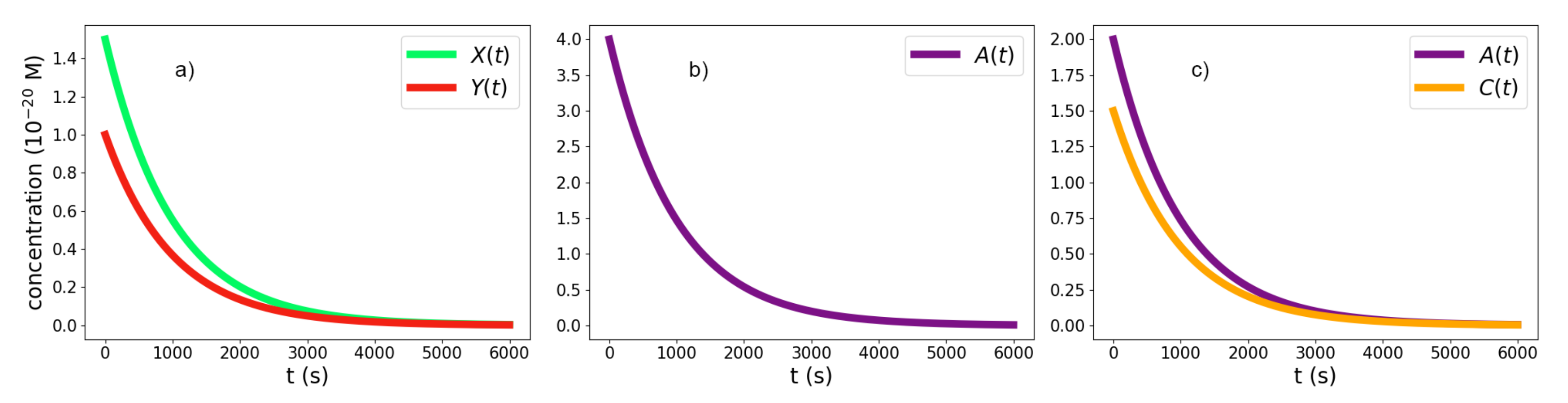
3.1. The Kinetic Study

A kinetic study is based on non-elementary approximation in order to model closed markets (when the price of products does not change for the analysed period). It is especially recommended if there are data available about the quantities of products sold and about the transactions in order to help calibrate the rates and rate constants of the chemical reactions. There are two limit cases discussed, in which either the product is in unlimited supply or the demand for the product is very high.

What we find is that the products and conventional money decrease exponentially over time when there are no tokens present in the system (RM1).

Introducing tokens as an additional means for selling products while keeping the conventional channels open as well (RM2) will not alter the profile of how the products are sold. Lowering the number of tokens on the market will slow down the rate of the chemical reaction involving tokens in comparison to a reaction that describes selling the same product but with conventional money only. A larger number of tokens will speed up the reaction describing the transactions involving tokens to the detriment of the reaction involving only conventional money.

When the system is designed such that a product can only be sold with a combination of conventional money and tokens (RM2s), the price of the product can be treated as a composite currency, and its profile will decrease exponentially over time as well.

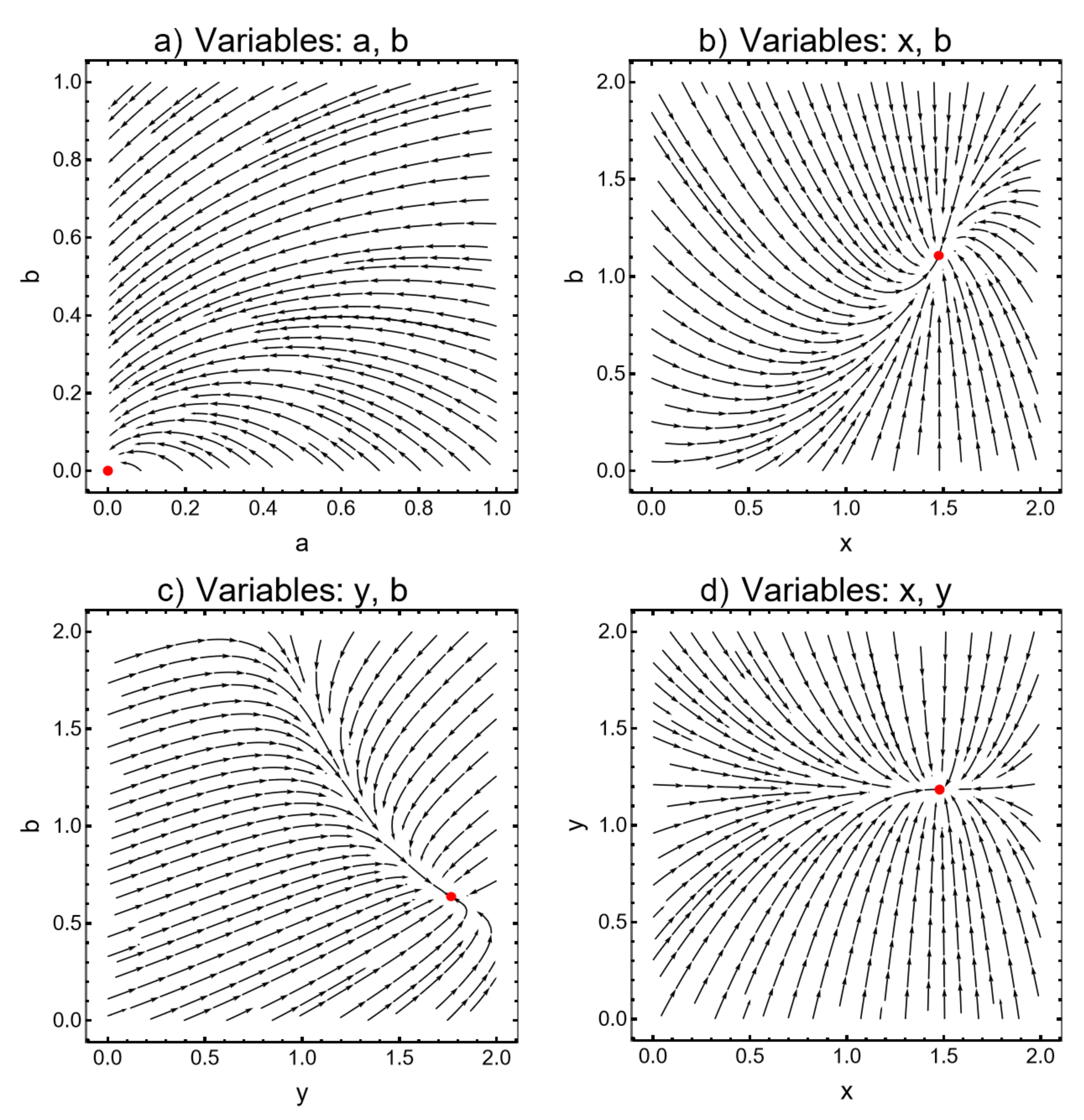
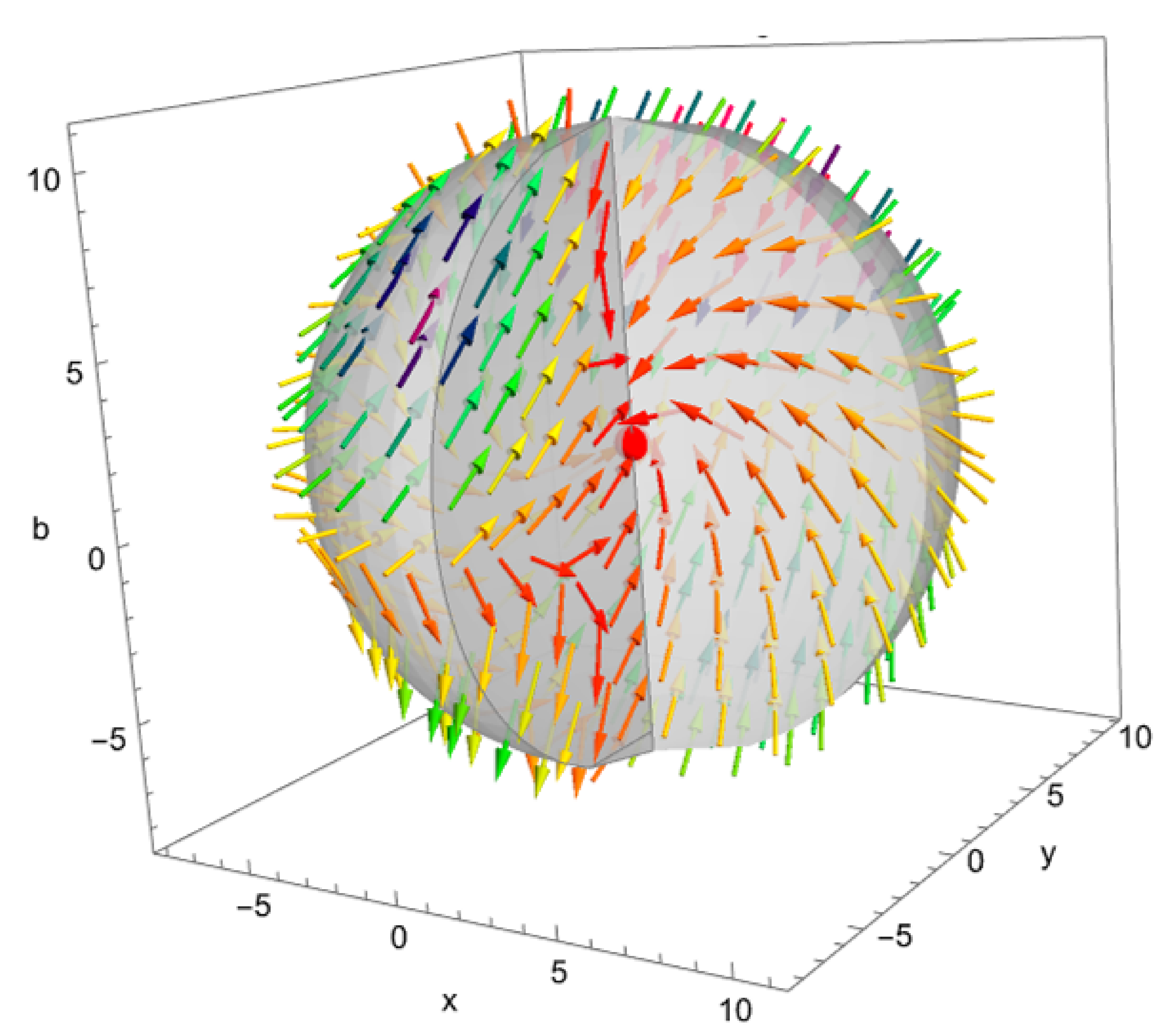
3.2. The Stability Analysis

A stability analysis is a dynamical model that reveals more general behaviour than the kinetic study. However, because it is based on an elementary assumption, it is not complementary to the kinetic study.

Analysing the directional fields around real positive fixed points reveals that for any set of ODEs (RM1, RM2, RM2s), the steady states are stable nodes, except for one saddle point. Ruling out any oscillatory or unstable behaviour for most of the cases, one can say with confidence that small perturbations around the equilibrium states of the ODE systems describing the chemical reactions will decrease monotonically. Even the runaway situation of the unstable equilibrium case seems to take place quite close to zero for two out of three components, making it unlikely to cause major disruptions.

3.3. Coefficient Adjustments

Adjusting coefficients according to the supply and demand law is a technique that is complementary to the previous two methods, and is applied to a sequence of closed-market instances. It consists of keeping the concentrations of the molecules constant while their coefficients vary in order to symbolise price variations according to the surplus or deficit of products.

Using the same chemical framework (even though applying this law has no connection to chemistry) reveals how the chemical model itself incorporates several token characteristics. If there are no tokens involved and two separate products are sold independently (RM1), the surplus or deficit of any product will have an impact only on its own price and will not influence the price of the other product. For any other system involving tokens (RM2 and RM2s), there are a series of token properties that have to be decided upon in advance: Do the tokens have subdivisions or are they granted and used as an indivisible unit? If they are used as a unit, how is the exchange rate between tokens and conventional money going to be calculated?

4. Discussion

The results of the kinetic study draw attention to the fact that small variations in the way an economic system is set up can have a significant impact on which product is sold faster or slower. It is important to have a sense of how transactions and sales are impacted when adding tokens in a practical sense in order to avoid business plans and expectations not matching reality. This also points out how even though conventional money and tokens are different in nature, from an analytical point of view, they can be treated as a composite currency under certain circumstances.

The key to introducing tokens successfully is a robust design of the token economy model [40,41]. However, the literature on this topic is still scarce [42], and a stability analysis from a chemical perspective has not been used in this context before. Even though we can only show an example of one unstable equilibrium in this paper, the possibility for purely unstable behaviour to surface when analysing different systems is not zero. Unstable behaviour in this context could mean a rapid increase in the demand for a product, which would increase its price unexpectedly, or could increase runaway inflation or the sudden unavailability of money, tokens, or products. In our future work, we plan to study the specific characteristics of systems that exhibit stable, oscillatory, or unstable behaviour and to understand what this means in terms of the ways that tokens are introduced in these systems. In the case of chaotic behaviour, control parameters can be identified [43,44], and if it turns out that tokens do have this influence, they can be seen as a stabilising factor in tokenised economic systems.

Applying the supply and demand laws to the chemical models with several degrees of token involvement shows a series of decisions that the architect of a tokenised model has to take into account. These decisions (divisible or unit tokens and token–money or token–token exchange rates [45,46]) might be intuitive for experts in the field. However, careful token design (and awareness of the token design space [47]) is crucial to the success of the new system. When tokens are not obtained and used in the way that they are intended (a weak design of token proofs can lead to individuals obtaining tokens illicitly), incentivising potentially malicious behaviour or choosing the wrong community for launching the tokenised systems can lead to a loss of trust in tokens (blockchain and digital technology) in general [47] and may harm the community.

The basis for policymaking, token design, and regulation is a cohesive and comprehensive taxonomy of token properties, along with classification models. The token behaviour that comes out of the chemical analysis environment, without any prior assumptions of token design, touches directly upon properties such as fungibility [48] (identical or non-identical tokens, interchangeability, and divisibility) and supply (fixed or unlimited supply). This shows that the chemical model does reliably account for such details. On the other hand, there are many more token properties that are relevant to the token design process, such as transferability, regulation, expiry date, and privacy. Moreover, token design relies not only on token properties, but also on technical, economic, legal, and ethical engineering [49]. In terms of policy, there are no unified guidelines for the token design process. At this stage, there are only isolated projects implementing and experimenting with token economies, and the rules of token design are made by trial and error. It is our belief that a system such as the demand and supply law in chemical context has the ability to standardise the need for establishing at least some of the token attributes.

In our future work, we intend to apply the stability tools described in this paper to a case study. The aim of the project is to reintroduce waste into the market by tokenising the system. We will explore the stability and the behaviour of a hybrid currency system in order to reduce waste and build a circular economy in the context of sustainability.

As quantified units of value, tokens can define a broader sense of value than conventional money, such as the value of natural or cultural capital [50]. We intend to analyse the ways in which tokens are obtained as incentives for the reintegration of waste and can be exchanged for cultural or social tokens.

5. Conclusions

The chemical framework and analytical methods proposed in this paper have the ability to deliver important information on short-term transaction profiles and the stability of an entire system, and even to anticipate the necessity of thorough token design.

By being a flexible and versatile model, it can be reduced or extended to fit the needs of almost any particular economic system—within the limits of the ideal gas assumption—and to capture its properties.

It is our belief that further research on this topic of chemical reaction mechanisms as models for hybrid economic systems has the potential to revolutionise the assessment and prediction of partially or fully tokenised markets. As one of the few methods existing today for objectively assessing sustainability and offering clear indications on token design, this chemical model could prove to be an invaluable framework for businesses interested in making the transition towards adopting systems that can be run on the blockchain, using cryptocurrency, and/or introducing tokens as incentives.

References

1. UN. Available online: https://www.un.org/sites/un2.un.org/files/un75_new_technologies.pdf (accessed on 2 July 2021).
2. UN. Available online: https://www.un.org/sites/un2.un.org/files/un75_final_report_shapingourfuturetogether.pdf (accessed on 2 July 2021).
3. Nadkarni, S.; Prügl, R. Digital transformation: A review, synthesis and opportunities for future research. Springer Manag. Rev. Q. 2021, 71, 233–341. [Google Scholar] [CrossRef] [Green Version]
4. Fitzgerald, M.; Kruschwitz, N.; Bonnet, D.; Welch, M. Embracing Digital Technology: A New Strategic Imperative. Mit Sloan Manag. Rev. 2013, 55, 1–13. [Google Scholar]
5. Ross, J.W.; Sebastian, I.M.; Beath, C.M.; Jha, L.; The Technology Advantage Practice of The Boston Consulting Group. MIT-CISR-Designing-Digital-Survey. Available online: https://media-publications.bcg.com/MIT-CISR-Designing-Digital-Survey.PDF (accessed on 5 July 2021).
6. Winden, W.; Carvalho, L. Cities and Digitalization. How Digitalization Changes Cities—Innovation for the Urban Economy of Tomorrow. Available online: https://www.business.ruhr/fileadmin/user_upload/Studie__Cities_and_digitalization__Euricur_wmr.pdf (accessed on 22 July 2021).
7. The Climate City Cup. Available online: https://climatecitycup.org (accessed on 22 July 2021).
8. Smart City: German Government Funding “Digital Twins” Project. Available online: https://hamburg-news.hamburg/en/location/smart-city-german-government-funding-digital-twins-project (accessed on 22 July 2021).
9. Gimpel, H.; Röglinger, M. Digital Transformation: Changes and Chances: Insights based on an Empirical Study. 2015. Available online: http://fim-rc.de/Paperbibliothek/Veroeffentlicht/542/wi-542.pdf (accessed on 2 July 2021).
10. Digital Trust & Security—Securing Digital Transformation. Available online: https://www.capgemini.com/de-de/wp-content/uploads/sites/5/2019/10/Securing-Digital-Transformation-Capgemini-Invent.pdf (accessed on 22 July 2021).
11. Swan, M. Blockchain: Blueprint for a New Economy; O’Reilly: Beijing, China, 2015. [Google Scholar]
12. Kirbac, G.; Tektas, B. The Role of Blockchain Technology in Ensuring Digital Transformation for Businesses: Advantages, Challenges and Application Steps. Proceedings 2021, 74, 17. [Google Scholar] [CrossRef]
13. Catalini, C.; Gans, J.S. Some Simple Economics of the Blockchain. NBER Work. Pap. 22952 2016. [Google Scholar] [CrossRef]
14. Hileman, G.; Rauchs, M. Global Cryptocurrency Benchmarking Study. Available online: https://www.jbs.cam.ac.uk/wp-content/uploads/2020/08/2017-04-20-global-cryptocurrency-benchmarking-study.pdf (accessed on 22 July 2021).
15. Lee, J.Y. A decentralised token economy: How blockchain and cryptocurencies can revolutionise business. Bus. Horizons 2019, 62, 773–784. [Google Scholar]
16. Mougayar, M. Tokenomics—A Business Guide to Token Usage, Utility and Value. Available online: https://medium.com/@wmougayar/tokenomics-a-business-guide-to-token-usage-utility-and-value-b19242053416 (accessed on 22 July 2021).
17. Matson, J.L.; Estabillo, J.; Matheis, M. Token Economy. Encycl. Personal. Individ. Differ. 2016, 1, 3. [Google Scholar]
18. Kleineberg, K.; Helbing, D. A “social bitcoin” could sustain a democratic digital world. Eur. Phys. J. Spec. Top. 2016, 225, 3231–3241. [Google Scholar] [CrossRef] [Green Version]
19. Dapp, M. Toward a Sustainable Circular Economy Powered by Community-Based Incentive Systems. InBusiness Transformation through Blockchain; Treiblmaier, H., Beck, R., Eds.; Palgrave Macmillan: Cham, Switzerland, 2019; pp. 153–181. [Google Scholar]
20. Commons Stack. Realigning Incentives around Public Goods. Available online: https://medium.com/commonsstack (accessed on 6 July 2021).
21. Treecycle. We are Fighting Illegal Deforestation by Transforming Fallow Lands into Fast-Growing Sustainable Forests. Available online: https://treecycle.ch/en/ (accessed on 6 July 2021).
22. Dusk Network: The Privacy Blockchain for Financial Applications. Available online: https://dusk.network/ (accessed on 6 July 2021).
23. Circles. A Basic Income on the Blockchain. Available online: https://joincircles.net/ (accessed on 6 July 2021).
24. Forbes: “Reddit Is Launching Ethereum Tokens For Its Subreddits”. Available online: https://www.forbes.com/sites/colinharper/2020/05/14/reddit-launches-ethereum-tokens-for-subbredits-in-new-community-points-campaign/ (accessed on 10 October 2021).
25. Tönnissen, S.; Beinke, J.H.; Teuteberg, F. Understanding token-based ecosystems—A taxonomy of blockchain-based business models of start-ups. Electron. Mark. 2020, 30, 307–323. [Google Scholar] [CrossRef] [Green Version]
26. Conley, J.P. Blockchain and the Economics of Crypto-tokens and Initial Coin Offerings; Vanderbilt University Department of Economics Working Papers; VUECON-17-00008; Vanderbilt University: Nashville, TN, USA, 2017; p. 37235. [Google Scholar]
27. Drasch, B.J.; Fridgen, G.; Manner-Romberg, T.; Nolting, F.M.; Radszuwill, S. The token’s secret: The two-faced financial incentive of the token economy. Electron. Mark. 2020, 30, 557–567. [Google Scholar] [CrossRef] [Green Version]
28. Victor, F.; Lüders, B.K. Measuring ethereum-based erc20 token networks. In International Conference on Financial Cryptography and Data Security; Springer: Cham, Switzerland, 2019; pp. 113–129. [Google Scholar]
29. Stanley, M.H.R.; Amaral, L.A.N.; Buldyrev, S.V.; Havlin, S.; Leschhorn, H.; Maass, P.; Salinger, M.A.; Stanley, H.E. Scaling behavior in the growth of companies. Nature 1996, 379, 804. [Google Scholar] [CrossRef]
30. Rosario, M.N.; Kertész, J. Focus on Statistical Physics Modeling in Economics and Finance. New J. Phys. 2011, 13, 25011. [Google Scholar]
31. Chen, S.; Li, S. Econophysics: Bridges over a Turbulent Current. arXiv 2011, arXiv:1107.5373. [Google Scholar] [CrossRef] [Green Version]
32. Kutnera, R.; Ausloos, M.; Grechc, D.; Di Matteo, T.; Schinckusg, C.; Stanley, H.E. Econophysics and sociophysics: Their milestones & challenges. Phys. Stat. Mech. Appl. 2019, 516, 240–253. [Google Scholar]
33. Helbing, D. Social Self-Organization. Agent-Based Simulations and Experiments to Study Emergent Social Behaviour; Springer: Heidelberg, Germany; New York, NY, USA; Dordrecht, The Netherlands; London, UK, 2012. [Google Scholar]
34. Yochanan, S.; Reuel, S. Do Chemical Reactors Hold the Solution for Global Economic Crises? PIER Working Paper No. 12-010; Penn Institute for Economic Research Department of Economics, University of Pennsylvania: Philadelphia, PA, USA, 2012. [Google Scholar]
35. Hartmann, G.C.; Rossler, O.E. Coupled Flare Attractors A Discrete Prototype for Economic Modelling. Discret. Dyn. Nat. Soc. 2012, 1998, 153–159. [Google Scholar]
36. Field, R.J. Chaos in the belousov-zhabotinsky reaction. Mod. Phys. Lett. B 2015, 29. [Google Scholar] [CrossRef]
37. Kol’tsov, N. Chaotic oscillations in four-step chemical reaction. Russ. J. Phys. Chem. B 2017, 11, 1047–1048. [Google Scholar] [CrossRef]
38. Epstein, I.R.; Pojman, J.A. An Introduction to Nonlinear Chemical Dynamics. Oscillations, Waves, Patterns and Chaos; Oxford University Press: New York, NY, USA; Oxford, UK, 1998. [Google Scholar]
39. Strogatz, S.H. Nonlinear Dynamics and Chaos; Perseus Books: Reading, MA, USA, 1994. [Google Scholar]
40. Kim, M.S.; Chung, J.Y. Sustainable growth and token economy design: The case of steemit. Sustainability 2019, 11, 167. [Google Scholar] [CrossRef] [Green Version]
41. Voshmgir, S. Token Economy—The Future of Currencies? Available online: https://medium.com/crypto3conomics/token-economy-the-future-of-currencies-d26487fd3945 (accessed on 10 October 2021).
42. Kampakis, S. Why do we need tokenomics? JBBA 2018, 1, 1–4. [Google Scholar] [CrossRef] [Green Version]
43. Lai, Y.; Gould, H.; Tobochnik, J. Controlling Chaos. Comput. Phys. 1994, 8, 62. [Google Scholar] [CrossRef] [Green Version]
44. Santos, R.B.B.; Graves, J.C. Extracting Chaos Control Parameters from Time Series Analysis. J. Phys. Conf. Ser. 2011, 285, 12002. [Google Scholar] [CrossRef]
45. Ballandies, M.C.; Dapp, M.M.; Pournaras, E. Decrypting distributed ledger design—Taxonomy, classification and blockchain community evaluation. Clust. Comput. 2021. [Google Scholar] [CrossRef]
46. Glatz, F. A Blockchain Token Taxonomy. Available online: https://medium.com/@heckerhut/a-blockchain-tokentaxonomy-fadf5c56139a (accessed on 10 October 2021).
47. Ballandies, M.C.; Dapp, M.M.; Degenhart, B.A.; Helbing, D.; Klauser, S.; Pardi, A. Finance 4.0—A Socio-Ecological Finance System. In Finance 4.0—Towards a Socio-Ecological Finance System; Dapp, M., Helbing, D., Klauser, S., Eds.; Springer: Cham, Switzerland, 2021; pp. 53–91. [Google Scholar]
48. Fungible vs. Non-Fungible Tokens on the Blockchain, 0xcert. Available online: https://medium.com/0xcert/fungible-vs-non-fungible-tokens-on-the-blockchain-ab4b12e0181a (accessed on 10 October 2021).
49. Voshmgir, S. Token Economy: How Blockchain & Smart Contracts Revolutionize the Economy; Token Kitchen: Berlin, Germany, 2019. [Google Scholar]
50. Helbing, D.; Klauser, S.; Dapp, M.; Ballandies, M.; Degenhart, B. FuturICT 2.0: Towards a Sustainable Digital Society with a Socio-Ecological Finance System (Finance 4.0); ETH: Zürich, Switzerland, 2020; Available online: ebook.finfour.net (accessed on 22 July 2021).
Figure 1. Time dependence of (a) X ( t ) and Y ( t ) for RM1 (left) calculated assuming the [ A ] [ Z ] case, (b) A ( t ) for the one-currency mechanism in RM1 (middle), and (c) A ( t ) , C ( t ) for RM2s (right), calculated considering the [ Z ] [ A ] case. The composite currency C ( t ) has the same time profile as that of the conventional currency A ( t ) .
Mathematics 09 02607 g001
Figure 2. Directional fields for (a) RM2 and RM2s a, b variable (upper left), (b) x and b variable (upper right), (c) y, b variable in RM2 (lower left), and (d) x, y variable (lower right). All of the plots depict stable nodes.
Mathematics 09 02607 g002
Figure 3. Directional fields for the ODEs of RM2 with x, y, and b being variable and a being fixed. The steady state is marked with a red sphere in the middle of the 3D plot. The region of interest is the lower part of the surface where the stream lines are coming out of the sphere.
Mathematics 09 02607 g003