A Study of Seven Asymmetric Kernels for the Estimation of Cumulative Distribution Functions

Abstract

In this paper, we complement a study recently conducted in a paper of H.A. Mombeni, B. Masouri and M.R. Akhoond by introducing five new asymmetric kernel c.d.f. estimators on the half-line $[0,\infty )$, namely the Gamma, inverse Gamma, LogNormal, inverse Gaussian and reciprocal inverse Gaussian kernel c.d.f. estimators. For these five new estimators, we prove the asymptotic normality and we find asymptotic expressions for the following quantities: bias, variance, mean squared error and mean integrated squared error. A numerical study then compares the performance of the five new c.d.f. estimators against traditional methods and the Birnbaum–Saunders and Weibull kernel c.d.f. estimators from Mombeni, Masouri and Akhoond. By using the same experimental design, we show that the LogNormal and Birnbaum–Saunders kernel c.d.f. estimators perform the best overall, while the other asymmetric kernel estimators are sometimes better but always at least competitive against the boundary kernel method from C. Tenreiro.

In the context of density estimation, asymmetric kernel estimators were introduced by Aitchison and Lauder [1] on the simplex and studied theoretically for the first time by Chen [2] on $[0,1]$ (using a Beta kernel), and by Chen [3] on $[0,\infty )$ (using a Gamma kernel). These estimators are designed so that the bulk of the kernel function varies with each point x in the support of the target density. More specifically, the parameters of the kernel function can vary in a way that makes the mode, the median or the mean equal to x. This variable smoothing allows asymmetric kernel estimators to behave better than traditional kernel estimators (see, e.g., Rosenblatt [4], Parzen [5]) near the boundary of the support in terms of their bias. Since the variable smoothing is integrated directly in the parametrization of the kernel function, asymmetric kernel estimators are also usually simpler to implement than boundary kernel methods (see, e.g., Gasser and Müller [6], Rice [7], Gasser et al. [8], Müller [9], Zhang and Karunamuni [10,11]). For these two reasons, asymmetric kernel estimators are, by now, well-known solutions to the boundary bias problem from which traditional kernel estimators suffer. In the past twenty years, various asymmetric kernels have been considered in the literature on density estimation:

• Beta kernel, when the target density is supported on $[0,1]$, see, e.g., Chen [2], Bouezmarni and Rolin [12], Renault and Scaillet [13], Fernandes and Monteiro [14], Hirukawa [15], Bouezmarni and Rombouts [16], Zhang and Karunamuni [17], Bertin and Klutchnikoff [18,19] Igarashi [20];
• Gamma, inverse Gamma, LogNormal, inverse Gaussian, reciprocal inverse Gaussian, Birnbaum–Saunders and Weibull kernels, when the target density is supported on $[0,\infty )$, see, e.g., Chen [3], Jin and Kawczak [21], Scaillet [22], Bouezmarni and Scaillet [23], Fernandes and Monteiro [14], Bouezmarni and Rombouts [16], fBouezmarni and Rombouts [24], Bouezmarni and Rombouts [25], Igarashi and Kakizawa [26,27], Charpentier and Flachaire [28], Igarashi [29], Zougab and Adjabi [30], Kakizawa and Igarashi [31], Kakizawa [32], Zougab et al. [33], Zhang [34], Kakizawa [35];
• Dirichlet kernel, when the target density is supported on the d-dimensional unit simplex, see [1] and the first theoretical study by Ouimet and Tolosana-Delgado [36].
• Continuous associated kernels, the aim of which is to unify the theory of asymmetric kernels with the one for traditional kernels in both the univariate and multivariate settings, see, e.g., Kokonendji and Libengué Dobélé-Kpoka [37], Kokonendji and Somé [38,39].

The interested reader is referred to Hirukawa [40] and Section 2 of Ouimet and Tolosana-Delgado [36] for a review of some of these papers and an extensive list of papers dealing with asymmetric kernels in other settings.

In contrast, there are almost no papers dealing with the estimation of cumulative distribution functions (c.d.f.s) in the literature on asymmetric kernels. In fact, to the best of our knowledge, [41] seems to be the first (and only) paper in this direction if we exclude the closely related theory of Bernstein estimators. (In the setting of Bernstein estimators, c.d.f. estimation on compact sets was tackled, for example, by Babu et al. [42], Leblanc [43], Leblanc [44], Leblanc [45], Dutta [46], Jmaei et al. [47], Erdoğan et al. [48] and Wang et al. [49] in the univariate setting, and by Babu and Chaubey [50], Belalia [51], Dib et al. [52] and Ouimet [53,54] in the multivariate setting. In [55], the authors introduced Bernstein estimators with Poisson weights (also called Szasz estimators) for the estimation of c.d.f.s that are supported on $[0,\infty )$, see also Ouimet [56]).

In the present paper, we complement the study reported in [41] by introducing five new asymmetric kernel c.d.f. estimators, namely the Gamma, inverse Gamma, LogNormal, inverse Gaussian and reciprocal inverse Gaussian kernel c.d.f. estimators. Our goal is to prove several asymptotic properties for these five new estimators (bias, variance, mean squared error, mean integrated squared error and asymptotic normality) and compare their numerical performance against traditional methods and against the Birnbaum–Saunders and Weibull kernel c.d.f. estimators from [41]. As we will see in the discussion of the results (Section 9), the LogNormal and Birnbaum–Saunders kernel c.d.f. estimators perform the best overall, while the other asymmetric kernel estimators are sometimes better but always at least competitive against the boundary kernel method from [57].

1. The Models

Let $X_1,X_2,\dots ,X_n$ be a sequence of i.i.d. observations from an unknown cumulative distribution function F supported on the half-line $[0,\infty )$. We consider the following seven asymmetric kernel estimators (the first five are new):

$$\begin{array}{cc}\hfill & {\widehat{F}}_{n,b}^{\mathrm{Gam}}\left(x\right)=\frac{1}{n}\sum _{i=1}^n{\overline{K}}_{\mathrm{Gam}}\left(X_i\right|b^{-1}x+1,b),\hfill \end{array}$$

(1)

$$\begin{array}{cc}\hfill & {\widehat{F}}_{n,b}^{\mathrm{IGam}}\left(x\right)=\frac{1}{n}\sum _{i=1}^n{\overline{K}}_{\mathrm{IGam}}\left(X_i\right|b^{-1}+1,x^{-1}b),\hfill \end{array}$$

(2)

$$\begin{array}{cc}\hfill & {\widehat{F}}_{n,b}^{\mathrm{LN}}\left(x\right)=\frac{1}{n}\sum _{i=1}^n{\overline{K}}_{\mathrm{LN}}\left(X_i\right|logx,\sqrt{b}),\hfill \end{array}$$

(3)

$$\begin{array}{cc}\hfill & {\widehat{F}}_{n,b}^{\mathrm{IGau}}\left(x\right)=\frac{1}{n}\sum _{i=1}^n{\overline{K}}_{\mathrm{IGau}}\left(X_i\right|x,b^{-1}x),\hfill \end{array}$$

(4)

$$\begin{array}{cc}\hfill & {\widehat{F}}_{n,b}^{\mathrm{RIG}}\left(x\right)=\frac{1}{n}\sum _{i=1}^n{\overline{K}}_{\mathrm{RIG}}\left(X_i\right|x^{-1}{(1-b)}^{-1},x^{-1}{b}^{-1}),\hfill \end{array}$$

(5)

$$\begin{array}{cc}\hfill & {\widehat{F}}_{n,b}^{\mathrm{B}-\mathrm{S}}\left(x\right)=\frac{1}{n}\sum _{i=1}^n{\overline{K}}_{\mathrm{B}-\mathrm{S}}\left(X_i\right|x,\sqrt{b}),\hfill \end{array}$$

(6)

$$\begin{array}{cc}\hfill & {\widehat{F}}_{n,b}^{\mathrm{W}}\left(x\right)=\frac{1}{n}\sum _{i=1}^n{\overline{K}}_{\mathrm{W}}\left(X_i\right|x/\Gamma (1+b),b^{-1}),\hfill \end{array}$$

(7)

where $b>0$ is a smoothing (or bandwidth) parameter, and

$$\begin{array}{cccc}& {\overline{K}}_{\mathrm{Gam}}\left(t\right|\alpha ,\theta )=\frac{\Gamma (\alpha ,t/\theta )}{\Gamma \left(\alpha \right)},\hfill & & \alpha ,\theta >0,\hfill \\ & {\overline{K}}_{\mathrm{IGam}}\left(t\right|\alpha ,\theta )=1-\frac{\Gamma (\alpha ,1/(t\theta \left)\right)}{\Gamma \left(\alpha \right)},\hfill & & \alpha ,\theta >0,\hfill \\ & {\overline{K}}_{\mathrm{LN}}\left(t\right|\mu ,\sigma )=1-\Phi \left(\frac{logt-\mu }{\sigma }\right),\hfill & & \mu ,\sigma >0,\hfill \\ & {\overline{K}}_{\mathrm{IGau}}\left(t\right|\mu ,\lambda )=1-\Phi \left(\sqrt{\frac{\lambda }{t}}\left(\frac{t}{\mu }-1\right)\right)-e^{2\lambda /\mu }\Phi \left(-\sqrt{\frac{\lambda }{t}}\left(\frac{t}{\mu }+1\right)\right),\hfill & & \mu ,\lambda >0,\hfill \\ & {\overline{K}}_{\mathrm{RIG}}\left(t\right|\mu ,\lambda )=\Phi \left(\sqrt{\lambda t}\left(\frac{1}{t\mu }-1\right)\right)+e^{2\lambda /\mu }\Phi \left(-\sqrt{\lambda t}\left(\frac{1}{t\mu }+1\right)\right),\hfill & & \mu ,\lambda >0,\hfill \\ & {\overline{K}}_{\mathrm{B}-\mathrm{S}}\left(t\right|\beta ,\alpha )=1-\Phi \left(\frac{1}{\alpha }\left(\sqrt{\frac{t}{\beta }}-\sqrt{\frac{\beta }{t}}\right)\right),\hfill & & \beta ,\alpha >0,\hfill \\ & {\overline{K}}_{\mathrm{W}}\left(t\right|\lambda ,k)=exp\left(-{\left(\frac{t}{\lambda }\right)}^k\right),\hfill & & \lambda ,k>0,\hfill \end{array}$$

denote, respectively, the survival function of the

• $\mathrm{Gamma}(\alpha ,\theta )$ distribution (with the shape/scale parametrization);
• $\mathrm{InverseGamma}(\alpha ,\theta )$ distribution (with the shape/scale parametrization);
• $\mathrm{LogNormal}(\mu ,\sigma )$ distribution;
• $\mathrm{InverseGaussian}(\mu ,\lambda )$ distribution;
• $\mathrm{ReciprocalInverseGaussian}(\mu ,\lambda )$ distribution;
• $\mathrm{Birnbaum}-\mathrm{Saunders}(\beta ,\alpha )$ distribution;
• $\mathrm{Weibull}(\lambda ,k)$ distribution.

The function $\Gamma (\alpha ,z)={\int }_z^{\infty }{t}^{\alpha -1}{e}^{-t}\mathrm{d}t$ denotes the upper incomplete gamma function (where $\Gamma \left(\alpha \right)=\Gamma (\alpha ,0)$), and $\Phi$ denotes the c.d.f. of the standard normal distribution. The parametrizations are chosen so that

• The mode of the kernel function in (1) is x;
• The median of the kernel function in (3) and (6) is x;
• The mean of the kernel function in (2), (4), (5) and (7) is x.

In this paper, we will compare the numerical performance of the above seven asymmetric kernel c.d.f. estimators against the following three traditional estimators (K here is the c.d.f. of a kernel function):

$$\begin{array}{cc}\hfill & {\widehat{F}}_{n,b}^{\mathrm{OK}}\left(x\right)=\frac{1}{n}\sum _{i=1}^{n}K\left(\frac{x-X_i}{b}\right),\hfill \end{array}$$

(8)

$$\begin{array}{cc}\hfill & {\widehat{F}}_{n,b}^{\mathrm{BK}}\left(x\right)=\frac{1}{n}\sum _{i=1}^n\left\{K\left(\frac{x-X_i}{b}\right){𝟙}_{[b,\infty )}\left(x\right)+K\left(\frac{x-X_i}{x}\right){𝟙}_{(0,b)}\left(x\right)\right\},\hfill \end{array}$$

(9)

$$\begin{array}{cc}\hfill & {\widehat{F}}_n^{\mathrm{EDF}}\left(x\right)=\frac{1}{n}\sum _{i=1}^n{𝟙}_{[X_i,\infty )}\left(x\right),\hfill \end{array}$$

(10)

which denote, respectively, the ordinary kernel (OK) c.d.f. estimator (from Tiago de Oliveira [58], Nadaraja [59] or Watson and Leadbetter [60]), the boundary kernel (BK) c.d.f. estimator (from Example 2.3 in [57]) and the empirical c.d.f. (EDF) estimator.

2. Outline, Assumptions and Notation

2.1. Outline

In Section 3, Section 4, Section 5, Section 6 and Section 7, the asymptotic normality, and the asymptotic expressions for the bias, variance, mean squared error (MSE) and mean integrated squared error (MISE), are stated for the $\mathrm{Gam}$, $\mathrm{IGam}$, $\mathrm{LN}$, $\mathrm{IGau}$ and $\mathrm{RIG}$ kernel c.d.f. estimators, respectively. The proofs can be found in Appendix A, Appendix B, Appendix C, Appendix D and Appendix E, respectively. Aside from the asymptotic normality (which can easily be deduced), these results were obtained for the Birnbaum–Saunders and Weibull kernel c.d.f. estimators in [41]. In Section 8, we compare the performance of all seven asymmetric kernel estimators above with the three traditional estimators $\mathrm{OK}$, $\mathrm{BK}$ and $\mathrm{EDF}$, defined in (8)–(10). A discussion of the results and our conclusion follow in Section 9 and Section 10. Technical calculations for the proofs of the asymptotic results are gathered in Appendix F.

2.2. Assumptions

Throughout the paper, we make the following two basic assumptions:

• The target c.d.f. F has two continuous and bounded derivatives;
• The smoothing (or bandwidth) parameter $b=b_n>0$ satisfies $b\to 0$ as $n\to \infty$.

2.3. Notation

Throughout the paper, the notation $u=\mathcal{O}\left(v\right)$ means that $lim\; sup|u/v|<C<\infty$ as $n\to \infty$. The positive constant C can depend on the target c.d.f. F, but no other variable unless explicitly written as a subscript. For example, if C depends on a given point $x\in (0,\infty )$, we would write $u={\mathcal{O}}_x\left(v\right)$. Similarly, the notation $u=\mathrm{o}\left(v\right)$ means that $lim|u/v|=0$ as $n\to \infty$. Subscripts indicate which parameters the convergence rate can depend on. The symbol $\mathcal{D}$ over an arrow ‘⟶’ will denote the convergence in law (or distribution).

3. Asymptotic Properties of the c.d.f. Estimator with Gam Kernel

In this section, we find the asymptotic properties of the Gamma ($\mathrm{Gam}$) kernel estimator defined in (1).

Lemma 1

(Bias and variance). For any given $x\in (0,\infty )$,

$$\begin{array}{cc}\hfill & \mathbb{B}\mathrm{ias}[{\widehat{F}}_{n,b}^{\mathrm{Gam}}\left(x\right)]=\mathbb{E}[{\widehat{F}}_{n,b}^{\mathrm{Gam}}\left(x\right)]-F\left(x\right)=b·(f\left(x\right)+\frac{x}{2}{f}^{\prime }\left(x\right))+{\mathrm{o}}_x\left(b\right),\hfill \end{array}$$

(11)

$$\begin{array}{cc}\hfill & \mathbb{V}\mathrm{ar}\left({\widehat{F}}_{n,b}^{\mathrm{Gam}}\left(x\right)\right)=n^{-1}F\left(x\right)(1-F\left(x\right))-n^{-1}{b}^{1/2}·\frac{\sqrt{x}f\left(x\right)}{\sqrt{\pi }}+{\mathcal{O}}_x\left(n^{-1}b\right).\hfill \end{array}$$

(12)

Corollary 1

(Mean squared error). For any given $x\in (0,\infty )$,

$$\begin{array}{cc}\hfill \mathrm{MSE}\left({\widehat{F}}_{n,b}^{\mathrm{Gam}}\left(x\right)\right)& =\mathbb{V}\mathrm{ar}\left({\widehat{F}}_{n,b}^{\mathrm{Gam}}\left(x\right)\right)+{\left(\mathbb{B}\mathrm{ias}[{\widehat{F}}_{n,b}^{\mathrm{Gam}}\left(x\right)]\right)}^2\hfill \\ \hfill & =n^{-1}F\left(x\right)(1-F\left(x\right))-n^{-1}{b}^{1/2}·\frac{\sqrt{x}f\left(x\right)}{\sqrt{\pi }}\hfill \\ \hfill & +b^2·{(f\left(x\right)+\frac{x}{2}{f}^{\prime }\left(x\right))}^2+{\mathcal{O}}_x\left(n^{-1}b\right)+{\mathrm{o}}_x\left(b^2\right).\hfill \end{array}$$

(13)

In particular, if $f\left(x\right)·(f\left(x\right)+x{f}^{\prime }\left(x\right))\ne 0$, the asymptotically optimal choice of b, with respect to $\mathrm{MSE}$, is

$$b_{\mathrm{opt}}=n^{-2/3}{\left[\frac{4·{(f\left(x\right)+\frac{x}{2}{f}^{\prime }\left(x\right))}^2}{\sqrt{x}f\left(x\right)/\sqrt{\pi }}\right]}^{-2/3}$$

(14)

with

$$\begin{array}{cc}\hfill \mathrm{MSE}\left({\widehat{F}}_{n,b_{\mathrm{opt}}}^{\mathrm{Gam}}\left(x\right)\right)& =n^{-1}F\left(x\right)(1-F\left(x\right))\hfill \\ \hfill & -n^{-4/3}\frac{3}{4}{\left[\frac{{(\sqrt{x}f\left(x\right)/\sqrt{\pi })}^4}{4·{(f\left(x\right)+\frac{x}{2}{f}^{\prime }\left(x\right))}^2}\right]}^{1/3}+{\mathrm{o}}_x\left(n^{-4/3}\right).\hfill \end{array}$$

(15)

Proposition 1

(Mean integrated squared error). Assuming that the target density $f=F^{\prime }$ satisfies

$${\int }_0^{\infty }\sqrt{x}f\left(x\right)\mathrm{d}x<\infty \mathit{and}{\int }_0^{\infty }{(f\left(x\right)+\frac{x}{2}{f}^{\prime }\left(x\right))}^2\mathrm{d}x<\infty ,$$

(16)

then we have

$$\begin{array}{cc}\hfill \mathrm{MISE}\left({\widehat{F}}_{n,b}^{\mathrm{Gam}}\right)& ={\int }_0^{\infty }\mathbb{V}\mathrm{ar}\left({\widehat{F}}_{n,b}^{\mathrm{Gam}}\left(x\right)\right)\mathrm{d}x+{\int }_0^{\infty }{\left(\mathbb{B}\mathrm{ias}[{\widehat{F}}_{n,b}^{\mathrm{Gam}}\left(x\right)]\right)}^2\mathrm{d}x\hfill \\ \hfill & =n^{-1}{\int }_0^{\infty }F\left(x\right)(1-F\left(x\right))\mathrm{d}x-n^{-1}{b}^{1/2}{\int }_0^{\infty }\frac{\sqrt{x}f\left(x\right)}{\sqrt{\pi }}\mathrm{d}x\hfill \\ \hfill & +b^2{\int }_0^{\infty }{(f\left(x\right)+\frac{x}{2}{f}^{\prime }\left(x\right))}^2\mathrm{d}x+\mathrm{o}\left(n^{-1}{b}^{1/2}\right)+\mathrm{o}\left(b^2\right).\hfill \end{array}$$

(17)

In particular, if $f\left(x\right)·(f\left(x\right)+x{f}^{\prime }\left(x\right))\ne 0$, the asymptotically optimal choice of b, with respect to $\mathrm{MISE}$, is

$$b_{\mathrm{opt}}=n^{-2/3}{\left[\frac{4{\int }_0^{\infty }{(f\left(x\right)+\frac{x}{2}{f}^{\prime }\left(x\right))}^2\mathrm{d}x}{{\int }_0^{\infty }\sqrt{x}f\left(x\right)/\sqrt{\pi }\mathrm{d}x}\right]}^{-2/3}$$

(18)

with

$$\begin{array}{cc}\hfill \mathrm{MISE}\left({\widehat{F}}_{n,b_{\mathrm{opt}}}^{\mathrm{Gam}}\right)& =n^{-1}{\int }_0^{\infty }F\left(x\right)(1-F\left(x\right))\mathrm{d}x\hfill \\ \hfill & -n^{-4/3}\frac{3}{4}{\left[\frac{{\left({\int }_0^{\infty }\sqrt{x}f\left(x\right)/\sqrt{\pi }\mathrm{d}x\right)}^4}{4{\int }_0^{\infty }{(f\left(x\right)+\frac{x}{2}{f}^{\prime }\left(x\right))}^2\mathrm{d}x}\right]}^{1/3}+\mathrm{o}\left(n^{-4/3}\right).\hfill \end{array}$$

(19)

Proposition 2

(Asymptotic normality). For any $x>0$ such that $0<F\left(x\right)<1$, we have the following convergence in distribution:

$$n^{1/2}({\widehat{F}}_{n,b}^{\mathrm{Gam}}\left(x\right)-\mathbb{E}[{\widehat{F}}_{n,b}^{\mathrm{Gam}}\left(x\right)])\stackrel{\mathcal{D}}{⟶}\mathcal{N}(0,{\sigma }^2\left(x\right)),\mathrm{as}b\to 0,n\to \infty ,$$

(20)

where ${\sigma }^2\left(x\right)=F\left(x\right)(1-F\left(x\right))$. In particular, Lemma 1 implies

$$\begin{array}{cccc}& n^{1/2}({\widehat{F}}_{n,b}^{\mathrm{Gam}}\left(x\right)-F\left(x\right))\stackrel{\mathcal{D}}{⟶}\mathcal{N}(0,{\sigma }^2\left(x\right)),\hfill & & \mathit{if}{n}^{1/2}b\to 0,\hfill \end{array}$$

(21)

$$\begin{array}{cccc}& n^{1/2}({\widehat{F}}_{n,b}^{\mathrm{Gam}}\left(x\right)-F\left(x\right))\stackrel{\mathcal{D}}{⟶}\mathcal{N}(\lambda ·(f\left(x\right)+\frac{x}{2}{f}^{\prime }\left(x\right)),{\sigma }^2\left(x\right)),\hfill & & \mathit{if}{n}^{1/2}b\to \lambda ,\hfill \end{array}$$

(22)

for any constant $\lambda >0$.

4. Asymptotic Properties of the c.d.f. Estimator with IGam Kernel

In this section, we find the asymptotic properties of the inverse Gamma ($\mathrm{IGam}$) kernel estimator defined in (2).

Lemma 2

(Bias and variance). For any given $x\in (0,\infty )$,

$$\mathbb{B}\mathrm{ias}[{\widehat{F}}_{n,b}^{\mathrm{IGam}}\left(x\right)]:=\mathbb{E}[{\widehat{F}}_{n,b}^{\mathrm{IGam}}\left(x\right)]-F\left(x\right)=b·\frac{x^2}{2}{f}^{\prime }\left(x\right)+{\mathrm{o}}_x\left(b\right),$$

(23)

$$\mathbb{V}\mathrm{ar}\left({\widehat{F}}_{n,b}^{\mathrm{IGam}}\left(x\right)\right)=n^{-1}F\left(x\right)(1-F\left(x\right))-n^{-1}{b}^{1/2}·\frac{xf\left(x\right)}{\sqrt{\pi }}+{\mathcal{O}}_x\left(n^{-1}b\right).$$

(24)

Corollary 2

(Mean squared error). For any given $x\in (0,\infty )$,

$$\begin{array}{cc}\hfill \mathrm{MSE}\left({\widehat{F}}_{n,b}^{\mathrm{IGam}}\left(x\right)\right)& =\mathbb{V}\mathrm{ar}\left({\widehat{F}}_{n,b}^{\mathrm{IGam}}\left(x\right)\right)+{\left(\mathbb{B}\mathrm{ias}[{\widehat{F}}_{n,b}^{\mathrm{IGam}}\left(x\right)]\right)}^2\hfill \\ \hfill & =n^{-1}F\left(x\right)(1-F\left(x\right))-n^{-1}{b}^{1/2}·\frac{xf\left(x\right)}{\sqrt{\pi }}\hfill \\ \hfill & +b^2·\frac{x^4}{4}{\left(f^{\prime }\left(x\right)\right)}^2+{\mathcal{O}}_x\left(n^{-1}b\right)+{\mathrm{o}}_x\left(b^2\right).\hfill \end{array}$$

(25)

In particular, if $f\left(x\right)·f^{\prime }\left(x\right)\ne 0$, the asymptotically optimal choice of b, with respect to $\mathrm{MSE}$, is

$$b_{\mathrm{opt}}=n^{-2/3}{\left[\frac{4·\frac{x^4}{4}{\left(f^{\prime }\left(x\right)\right)}^2}{xf\left(x\right)/\sqrt{\pi }}\right]}^{-2/3}$$

(26)

with

$$\begin{array}{cc}\hfill \mathrm{MSE}\left({\widehat{F}}_{n,b_{\mathrm{opt}}}^{\mathrm{IGam}}\left(x\right)\right)& =n^{-1}F\left(x\right)(1-F\left(x\right))\hfill \\ \hfill & -n^{-4/3}\frac{3}{4}{\left[\frac{{\left(xf\left(x\right)/\sqrt{\pi }\right)}^4}{4·\frac{x^4}{4}{\left(f^{\prime }\left(x\right)\right)}^2}\right]}^{1/3}+{\mathrm{o}}_x\left(n^{-4/3}\right).\hfill \end{array}$$

(27)

Proposition 3

(Mean integrated squared error). Assuming that the target density $f=F^{\prime }$ satisfies

$${\int }_0^{\infty }xf\left(x\right)\mathrm{d}x<\infty \mathit{and}{\int }_0^{\infty }{x}^4{\left(f^{\prime }\left(x\right)\right)}^2\mathrm{d}x<\infty ,$$

(28)

then we have

$$\begin{array}{cc}\hfill \mathrm{MISE}\left({\widehat{F}}_{n,b}^{\mathrm{IGam}}\right)& ={\int }_0^{\infty }\mathbb{V}\mathrm{ar}\left({\widehat{F}}_{n,b}^{\mathrm{IGam}}\left(x\right)\right)\mathrm{d}x+{\int }_0^{\infty }{\left(\mathbb{B}\mathrm{ias}[{\widehat{F}}_{n,b}^{\mathrm{IGam}}\left(x\right)]\right)}^2\mathrm{d}x\hfill \\ \hfill & =n^{-1}{\int }_0^{\infty }F\left(x\right)(1-F\left(x\right))\mathrm{d}x-n^{-1}{b}^{1/2}{\int }_0^{\infty }\frac{xf\left(x\right)}{\sqrt{\pi }}\mathrm{d}x\hfill \\ \hfill & +b^2{\int }_0^{\infty }\frac{x^4}{4}{\left(f^{\prime }\left(x\right)\right)}^2\mathrm{d}x+\mathrm{o}\left(n^{-1}{b}^{1/2}\right)+\mathrm{o}\left(b^2\right).\hfill \end{array}$$

(29)

In particular, if ${\int }_0^{\infty }{x}^4{\left(f^{\prime }\left(x\right)\right)}^2\mathrm{d}x>0$, the asymptotically optimal choice of b, with respect to $\mathrm{MISE}$, is

$$b_{\mathrm{opt}}=n^{-2/3}{\left[\frac{4{\int }_0^{\infty }\frac{x^4}{4}{\left(f^{\prime }\left(x\right)\right)}^2\mathrm{d}x}{{\int }_0^{\infty }xf\left(x\right)/\sqrt{\pi }\mathrm{d}x}\right]}^{-2/3}$$

(30)

with

$$\begin{array}{cc}\hfill \mathrm{MISE}\left({\widehat{F}}_{n,b_{\mathrm{opt}}}^{\mathrm{IGam}}\right)& =n^{-1}{\int }_0^{\infty }F\left(x\right)(1-F\left(x\right))\mathrm{d}x\hfill \\ \hfill & -n^{-4/3}\frac{3}{4}{\left[\frac{{\left({\int }_0^{\infty }xf\left(x\right)/\sqrt{\pi }\mathrm{d}x\right)}^4}{4{\int }_0^{\infty }\frac{x^4}{4}{\left(f^{\prime }\left(x\right)\right)}^2\mathrm{d}x}\right]}^{1/3}+\mathrm{o}\left(n^{-4/3}\right).\hfill \end{array}$$

(31)

Proposition 4

(Asymptotic normality). For any $x>0$ such that $0<F\left(x\right)<1$, we have the following convergence in distribution:

$$n^{1/2}({\widehat{F}}_{n,b}^{\mathrm{IGam}}\left(x\right)-\mathbb{E}[{\widehat{F}}_{n,b}^{\mathrm{IGam}}\left(x\right)])\stackrel{\mathcal{D}}{⟶}\mathcal{N}(0,{\sigma }^2\left(x\right)),asb\to 0,n\to \infty ,$$

(32)

where ${\sigma }^2\left(x\right)=F\left(x\right)(1-F\left(x\right))$. In particular, Lemma 2 implies

$$\begin{array}{cccc}& n^{1/2}({\widehat{F}}_{n,b}^{\mathrm{IGam}}\left(x\right)-F\left(x\right))\stackrel{\mathcal{D}}{⟶}\mathcal{N}(0,{\sigma }^2\left(x\right)),\hfill & & if{n}^{1/2}b\to 0,\hfill \end{array}$$

(33)

$$\begin{array}{cccc}& n^{1/2}({\widehat{F}}_{n,b}^{\mathrm{IGam}}\left(x\right)-F\left(x\right))\stackrel{\mathcal{D}}{⟶}\mathcal{N}(\lambda ·\frac{x^2{f}^{\prime }\left(x\right)}{2},{\sigma }^2\left(x\right)),\hfill & & if{n}^{1/2}b\to \lambda ,\hfill \end{array}$$

(34)

for any constant $\lambda >0$.

5. Asymptotic Properties of the c.d.f. Estimator with LN Kernel

In this section, we find the asymptotic properties of the LogNormal (LN) kernel estimator defined in (3).

Lemma 3

(Bias and variance). For any given $x\in (0,\infty )$,

$$\begin{array}{cc}\hfill & \mathbb{B}\mathrm{ias}[{\widehat{F}}_{n,b}^{\mathrm{LN}}\left(x\right)]:=\mathbb{E}[{\widehat{F}}_{n,b}^{\mathrm{LN}}\left(x\right)]-F\left(x\right)=b·\frac{x}{2}(f\left(x\right)+x{f}^{\prime }\left(x\right))+{\mathrm{o}}_x\left(b\right),\hfill \end{array}$$

(35)

$$\begin{array}{cc}\hfill & \mathbb{V}\mathrm{ar}\left({\widehat{F}}_{n,b}^{\mathrm{LN}}\left(x\right)\right)=n^{-1}F\left(x\right)(1-F\left(x\right))-n^{-1}{b}^{1/2}·\frac{xf\left(x\right)}{\sqrt{\pi }}+{\mathcal{O}}_x\left(n^{-1}b\right).\hfill \end{array}$$

(36)

Corollary 3

(Mean squared error). For any given $x\in (0,\infty )$,

$$\begin{array}{cc}\hfill \mathrm{MSE}\left({\widehat{F}}_{n,b}^{\mathrm{LN}}\left(x\right)\right)& =\mathbb{V}\mathrm{ar}\left({\widehat{F}}_{n,b}^{\mathrm{LN}}\left(x\right)\right)+{\left(\mathbb{B}\mathrm{ias}[{\widehat{F}}_{n,b}^{\mathrm{LN}}\left(x\right)]\right)}^2\hfill \\ \hfill & =n^{-1}F\left(x\right)(1-F\left(x\right))-n^{-1}{b}^{1/2}·\frac{xf\left(x\right)}{\sqrt{\pi }}\hfill \\ \hfill & +b^2·\frac{x^2}{4}{(f\left(x\right)+x{f}^{\prime }\left(x\right))}^2+{\mathcal{O}}_x\left(n^{-1}b\right)+{\mathrm{o}}_x\left(b^2\right).\hfill \end{array}$$

(37)

In particular, if $f\left(x\right)·(f\left(x\right)+x{f}^{\prime }\left(x\right))\ne 0$, the asymptotically optimal choice of b, with respect to $\mathrm{MSE}$, is

$$b_{\mathrm{opt}}=n^{-2/3}{\left[\frac{4·\frac{x^2}{4}{(f\left(x\right)+x{f}^{\prime }\left(x\right))}^2}{xf\left(x\right)/\sqrt{\pi }}\right]}^{-2/3}$$

(38)

with

$$\begin{array}{cc}\hfill \mathrm{MSE}\left({\widehat{F}}_{n,b_{\mathrm{opt}}}^{\mathrm{LN}}\left(x\right)\right)& =n^{-1}F\left(x\right)(1-F\left(x\right))\hfill \\ \hfill & -n^{-4/3}\frac{3}{4}{\left[\frac{{(xf\left(x\right)/\sqrt{\pi })}^4}{4·\frac{x^2}{4}{(f\left(x\right)+x{f}^{\prime }\left(x\right))}^2}\right]}^{1/3}+{\mathrm{o}}_x\left(n^{-4/3}\right).\hfill \end{array}$$

(39)

Proposition 5

(Mean integrated squared error). Assuming that the target density $f=F^{\prime }$ satisfies

$${\int }_0^{\infty }xf\left(x\right)\mathrm{d}x<\infty and{\int }_0^{\infty }{x}^2{(f\left(x\right)+x{f}^{\prime }\left(x\right))}^2\mathrm{d}x<\infty ,$$

(40)

then we have

$$\begin{array}{cc}\hfill \mathrm{MISE}\left({\widehat{F}}_{n,b}^{\mathrm{LN}}\right)& ={\int }_0^{\infty }\mathbb{V}\mathrm{ar}\left({\widehat{F}}_{n,b}^{\mathrm{LN}}\left(x\right)\right)\mathrm{d}x+{\int }_0^{\infty }{\left(\mathbb{B}\mathrm{ias}[{\widehat{F}}_{n,b}^{\mathrm{LN}}\left(x\right)]\right)}^2\mathrm{d}x\hfill \\ \hfill & =n^{-1}{\int }_0^{\infty }F\left(x\right)(1-F\left(x\right))\mathrm{d}x-n^{-1}{b}^{1/2}{\int }_0^{\infty }\frac{xf\left(x\right)}{\sqrt{\pi }}\mathrm{d}x\hfill \\ \hfill & +b^2{\int }_0^{\infty }\frac{x^2}{4}{(f\left(x\right)+x{f}^{\prime }\left(x\right))}^2\mathrm{d}x+\mathrm{o}\left(n^{-1}{b}^{1/2}\right)+\mathrm{o}\left(b^2\right).\hfill \end{array}$$

(41)

In particular, if $f\left(x\right)·(f\left(x\right)+x{f}^{\prime }\left(x\right))\ne 0$, the asymptotically optimal choice of b, with respect to $\mathrm{MISE}$, is

$$b_{\mathrm{opt}}=n^{-2/3}{\left[\frac{4{\int }_0^{\infty }\frac{x^2}{4}{(f\left(x\right)+x{f}^{\prime }\left(x\right))}^2\mathrm{d}x}{{\int }_0^{\infty }xf\left(x\right)/\sqrt{\pi }\mathrm{d}x}\right]}^{-2/3}$$

(42)

with

$$\begin{array}{cc}\hfill \mathrm{MISE}\left({\widehat{F}}_{n,b_{\mathrm{opt}}}^{\mathrm{LN}}\right)& =n^{-1}{\int }_0^{\infty }F\left(x\right)(1-F\left(x\right))\mathrm{d}x\hfill \\ \hfill & -n^{-4/3}\frac{3}{4}{\left[\frac{{\left({\int }_0^{\infty }xf\left(x\right)/\sqrt{\pi }\mathrm{d}x\right)}^4}{4{\int }_0^{\infty }\frac{x^2}{4}{(f\left(x\right)+x{f}^{\prime }\left(x\right))}^2\mathrm{d}x}\right]}^{1/3}+\mathrm{o}\left(n^{-4/3}\right).\hfill \end{array}$$

(43)

Proposition 6

(Asymptotic normality). For any $x>0$ such that $0<F\left(x\right)<1$, we have the following convergence in distribution:

$$n^{1/2}({\widehat{F}}_{n,b}^{\mathrm{LN}}\left(x\right)-\mathbb{E}[{\widehat{F}}_{n,b}^{\mathrm{LN}}\left(x\right)])\stackrel{\mathcal{D}}{⟶}\mathcal{N}(0,{\sigma }^2\left(x\right)),asb\to 0,n\to \infty ,$$

(44)

where ${\sigma }^2\left(x\right):=F\left(x\right)(1-F\left(x\right))$. In particular, Lemma 3 implies

$$\begin{array}{cccc}& n^{1/2}({\widehat{F}}_{n,b}^{\mathrm{LN}}\left(x\right)-F\left(x\right))\stackrel{\mathcal{D}}{⟶}\mathcal{N}(0,{\sigma }^2\left(x\right)),\hfill & & if{n}^{1/2}b\to 0,\hfill \end{array}$$

(45)

$$\begin{array}{cccc}& n^{1/2}({\widehat{F}}_{n,b}^{\mathrm{LN}}\left(x\right)-F\left(x\right))\stackrel{\mathcal{D}}{⟶}\mathcal{N}(\lambda ·\frac{x}{2}(f\left(x\right)+x{f}^{\prime }\left(x\right)),{\sigma }^2\left(x\right)),\hfill & & if{n}^{1/2}b\to \lambda ,\hfill \end{array}$$

(46)

for any constant $\lambda >0$.

6. Asymptotic Properties of the c.d.f. Estimator with IGau Kernel

In this section, we find the asymptotic properties of the inverse Gaussian (IGau) kernel estimator defined in ().

Lemma 4

(Bias and variance). For any given $x\in (0,\infty )$,

$$\mathbb{B}\mathrm{ias}[{\widehat{F}}_{n,b}^{\mathrm{IGau}}\left(x\right)]:=\mathbb{E}[{\widehat{F}}_{n,b}^{\mathrm{IGau}}\left(x\right)]-F\left(x\right)=b·\frac{x^2}{2}{f}^{\prime }\left(x\right)+{\mathrm{o}}_x\left(b\right),$$

(47)

$$\begin{array}{cc}\hfill \mathbb{V}\mathrm{ar}\left({\widehat{F}}_{n,b}^{\mathrm{IGau}}\left(x\right)\right)& =n^{-1}F\left(x\right)(1-F\left(x\right))-n^{-1}{b}^{1/2}·\frac{f\left(x\right)}{2}\left[\underset{b\to 0}{lim}{b}^{-1/2}\mathbb{E}[|T_1-T_2|]\right]\hfill \\ \hfill & +{\mathcal{O}}_x\left(n^{-1}b\right),\hfill \end{array}$$

(48)

where $T_1,T_2\stackrel{\mathrm{i}.\mathrm{i}.\mathrm{d}.}{\sim }\mathrm{IGau}(x,b^{-1}x)$.

Corollary 4

(Mean squared error). For any given $x\in (0,\infty )$,

$$\begin{array}{cc}\hfill \mathrm{MSE}\left({\widehat{F}}_{n,b}^{\mathrm{IGau}}\left(x\right)\right)& =\mathbb{V}\mathrm{ar}\left({\widehat{F}}_{n,b}^{\mathrm{IGau}}\left(x\right)\right)+{\left(\mathbb{B}\mathrm{ias}[{\widehat{F}}_{n,b}^{\mathrm{IGau}}\left(x\right)]\right)}^2\hfill \\ \hfill & =n^{-1}F\left(x\right)(1-F\left(x\right))-n^{-1}{b}^{1/2}·\frac{f\left(x\right)}{2}\left[\underset{b\to 0}{lim}{b}^{-1/2}\mathbb{E}[|T_1-T_2|]\right]\hfill \\ \hfill & +b^2·\frac{x^4}{4}{\left(f^{\prime }\left(x\right)\right)}^2+{\mathcal{O}}_x\left(n^{-1}b\right)+{\mathrm{o}}_x\left(b^2\right),\hfill \end{array}$$

(49)

where $T_1,T_2\stackrel{\mathrm{i}.\mathrm{i}.\mathrm{d}.}{\sim }\mathrm{IGau}(x,b^{-1}x)$. The quantity ${lim}_{b\to 0}{b}^{-1/2}\mathbb{E}[|T_1-T_2|]$ needs to be approximated numerically. In particular, if $f\left(x\right)\left[{lim}_{b\to 0}{b}^{-1/2}\mathbb{E}[|T_1-T_2|]\right]·f^{\prime }\left(x\right)\ne 0$, the asymptotically optimal choice of b, with respect to $\mathrm{MSE}$, is

$$b_{\mathrm{opt}}=n^{-2/3}{\left[\frac{4·\frac{x^4}{4}{\left(f^{\prime }\left(x\right)\right)}^2}{\frac{f\left(x\right)}{2}{lim}_{b\to 0}{b}^{-1/2}\mathbb{E}[|T_1-T_2|]}\right]}^{-2/3}$$

(50)

with

$$\begin{array}{cc}\hfill \mathrm{MSE}\left({\widehat{F}}_{n,b_{\mathrm{opt}}}^{\mathrm{IGau}}\left(x\right)\right)& =n^{-1}F\left(x\right)(1-F\left(x\right))\hfill \\ \hfill & -n^{-4/3}\frac{3}{4}{\left[\frac{{\left(\frac{f\left(x\right)}{2}{lim}_{b\to 0}{b}^{-1/2}\mathbb{E}[|T_1-T_2|]\right)}^4}{4·\frac{x^4}{4}{\left(f^{\prime }\left(x\right)\right)}^2}\right]}^{1/3}+{\mathrm{o}}_x\left(n^{-4/3}\right).\hfill \end{array}$$

(51)

Proposition 7

(Mean integrated squared error). Assuming that the target density $f=F^{\prime }$ satisfies

$${\int }_0^{\infty }f\left(x\right)\left[\underset{b\to 0}{lim}{b}^{-1/2}\mathbb{E}[|T_1-T_2|]\right]\mathrm{d}x<\infty and{\int }_0^{\infty }{x}^4{\left(f^{\prime }\left(x\right)\right)}^2\mathrm{d}x<\infty ,$$

(52)

where $T_1,T_2\stackrel{\mathrm{i}.\mathrm{i}.\mathrm{d}.}{\sim }\mathrm{IGau}(x,b^{-1}x)$, then we have

$$\begin{array}{cc}\hfill \mathrm{MISE}\left({\widehat{F}}_{n,b}^{\mathrm{IGau}}\right)& ={\int }_0^{\infty }\mathbb{V}\mathrm{ar}\left({\widehat{F}}_{n,b}^{\mathrm{IGau}}\left(x\right)\right)\mathrm{d}x+{\int }_0^{\infty }{\left(\mathbb{B}\mathrm{ias}[{\widehat{F}}_{n,b}^{\mathrm{IGau}}\left(x\right)]\right)}^2\mathrm{d}x\hfill \\ \hfill & =n^{-1}{\int }_0^{\infty }F\left(x\right)(1-F\left(x\right))\mathrm{d}x\hfill \\ \hfill & -n^{-1}{b}^{1/2}{\int }_0^{\infty }\frac{f\left(x\right)}{2}\left[\underset{b\to 0}{lim}{b}^{-1/2}\mathbb{E}[|T_1-T_2|]\right]\mathrm{d}x\hfill \\ \hfill & +b^2{\int }_0^{\infty }\frac{x^4}{4}{\left(f^{\prime }\left(x\right)\right)}^2\mathrm{d}x+\mathrm{o}\left(n^{-1}{b}^{1/2}\right)+\mathrm{o}\left(b^2\right).\hfill \end{array}$$

(53)

The quantity ${lim}_{b\to 0}{b}^{-1/2}\mathbb{E}[|T_1-T_2|]$ needs to be approximated numerically. In particular, if ${\int }_0^{\infty }{x}^4{\left(f^{\prime }\left(x\right)\right)}^2\mathrm{d}x>0$, the asymptotically optimal choice of b, with respect to $\mathrm{MISE}$, is

$$b_{\mathrm{opt}}=n^{-2/3}{\left[\frac{4{\int }_0^{\infty }\frac{x^4}{4}{\left(f^{\prime }\left(x\right)\right)}^2\mathrm{d}x}{{\int }_0^{\infty }\frac{f\left(x\right)}{2}{lim}_{b\to 0}{b}^{-1/2}\mathbb{E}[|T_1-T_2|]\mathrm{d}x}\right]}^{-2/3}$$

(54)

with

$$\begin{array}{cc}\hfill \mathrm{MISE}\left({\widehat{F}}_{n,b_{\mathrm{opt}}}^{\mathrm{IGau}}\right)& =n^{-1}{\int }_0^{\infty }F\left(x\right)(1-F\left(x\right))\mathrm{d}x\hfill \\ \hfill & -n^{-4/3}\frac{3}{4}{\left[\frac{{\left({\int }_0^{\infty }\frac{f\left(x\right)}{2}{lim}_{b\to 0}{b}^{-1/2}\mathbb{E}[|T_1-T_2|]\mathrm{d}x\right)}^4}{4{\int }_0^{\infty }\frac{x^4}{4}{\left(f^{\prime }\left(x\right)\right)}^2\mathrm{d}x}\right]}^{1/3}\hfill \\ \hfill & +\mathrm{o}\left(n^{-4/3}\right).\hfill \end{array}$$

(55)

Proposition 8

(Asymptotic normality). For any $x>0$ such that $0<F\left(x\right)<1$, we have the following convergence in distribution:

$$n^{1/2}({\widehat{F}}_{n,b}^{\mathrm{IGau}}\left(x\right)-\mathbb{E}[{\widehat{F}}_{n,b}^{\mathrm{IGau}}\left(x\right)])\stackrel{\mathcal{D}}{⟶}\mathcal{N}(0,{\sigma }^2\left(x\right)),\mathit{as}b\to 0,n\to \infty ,$$

(56)

where ${\sigma }^2\left(x\right)=F\left(x\right)(1-F\left(x\right))$. In particular, Lemma 4 implies

$$\begin{array}{cccc}& n^{1/2}({\widehat{F}}_{n,b}^{\mathrm{IGau}}\left(x\right)-F\left(x\right))\stackrel{\mathcal{D}}{⟶}\mathcal{N}(0,{\sigma }^2\left(x\right)),\hfill & & if{n}^{1/2}b\to 0,\hfill \end{array}$$

(57)

$$\begin{array}{cccc}& n^{1/2}({\widehat{F}}_{n,b}^{\mathrm{IGau}}\left(x\right)-F\left(x\right))\stackrel{\mathcal{D}}{⟶}\mathcal{N}(\lambda ·\frac{x^2}{2}{f}^{\prime }\left(x\right),{\sigma }^2\left(x\right)),\hfill & & if{n}^{1/2}b\to \lambda ,\hfill \end{array}$$

(58)

for any constant $\lambda >0$.

7. Asymptotic Properties of the c.d.f. Estimator with RIG Kernel

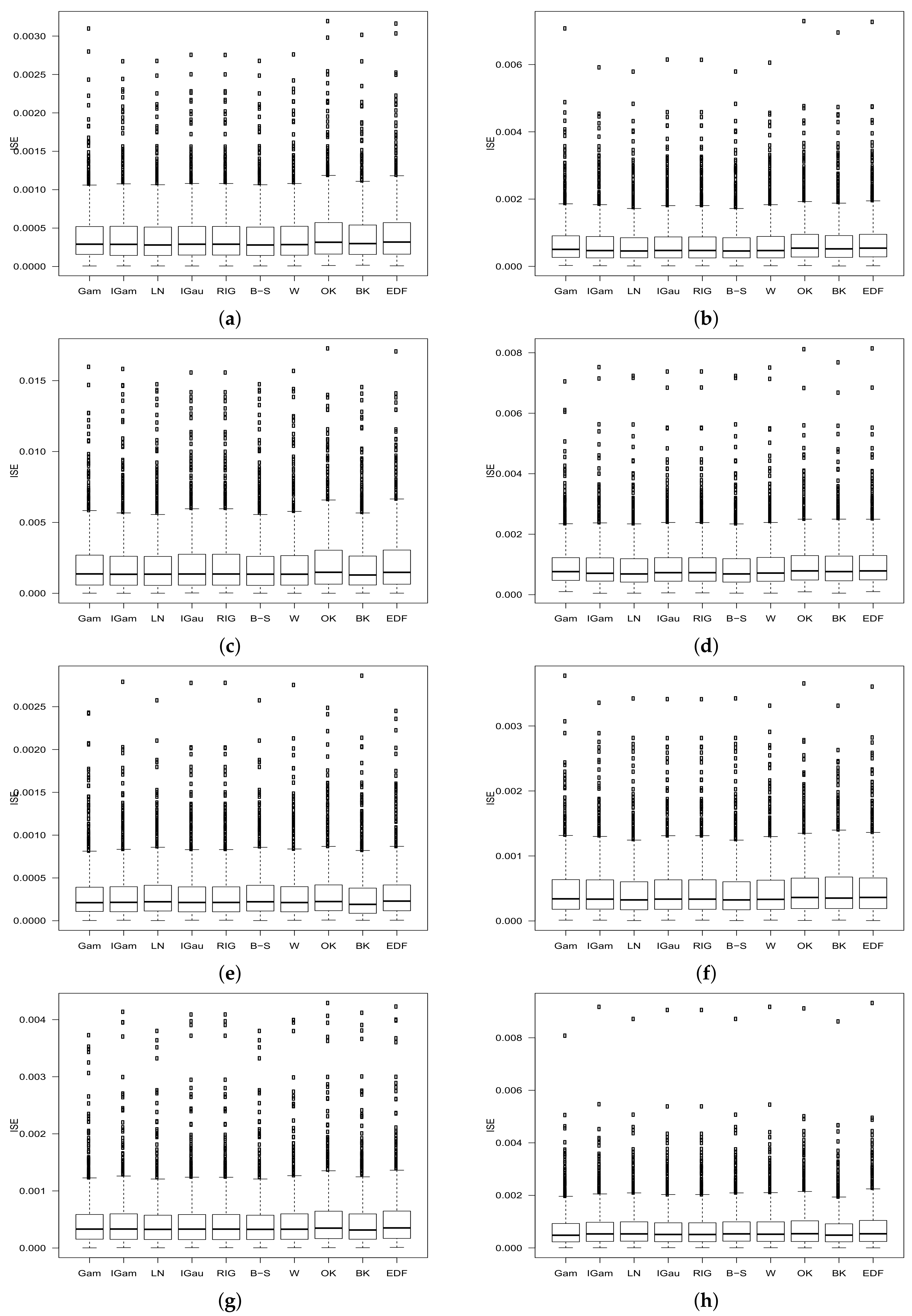
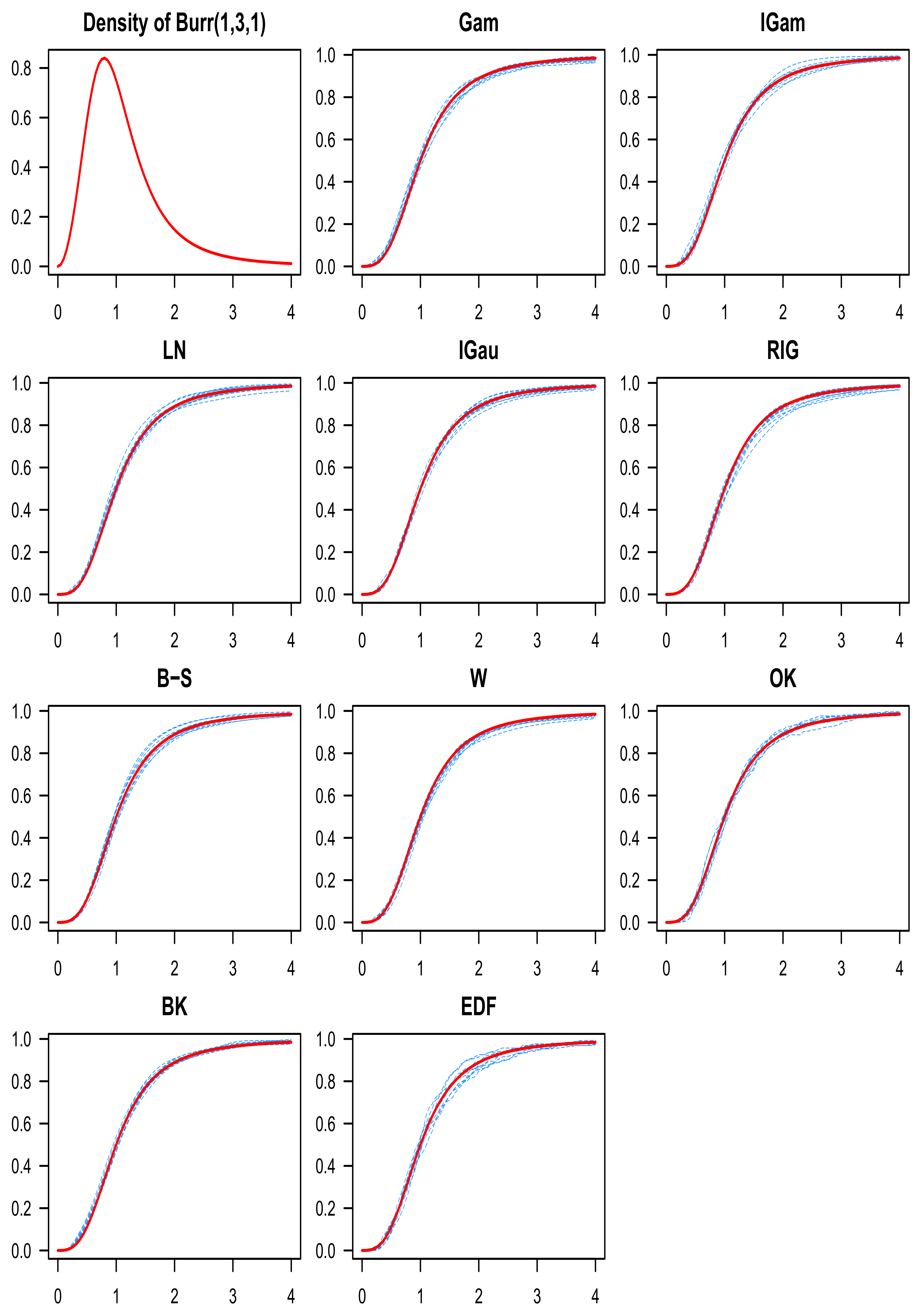
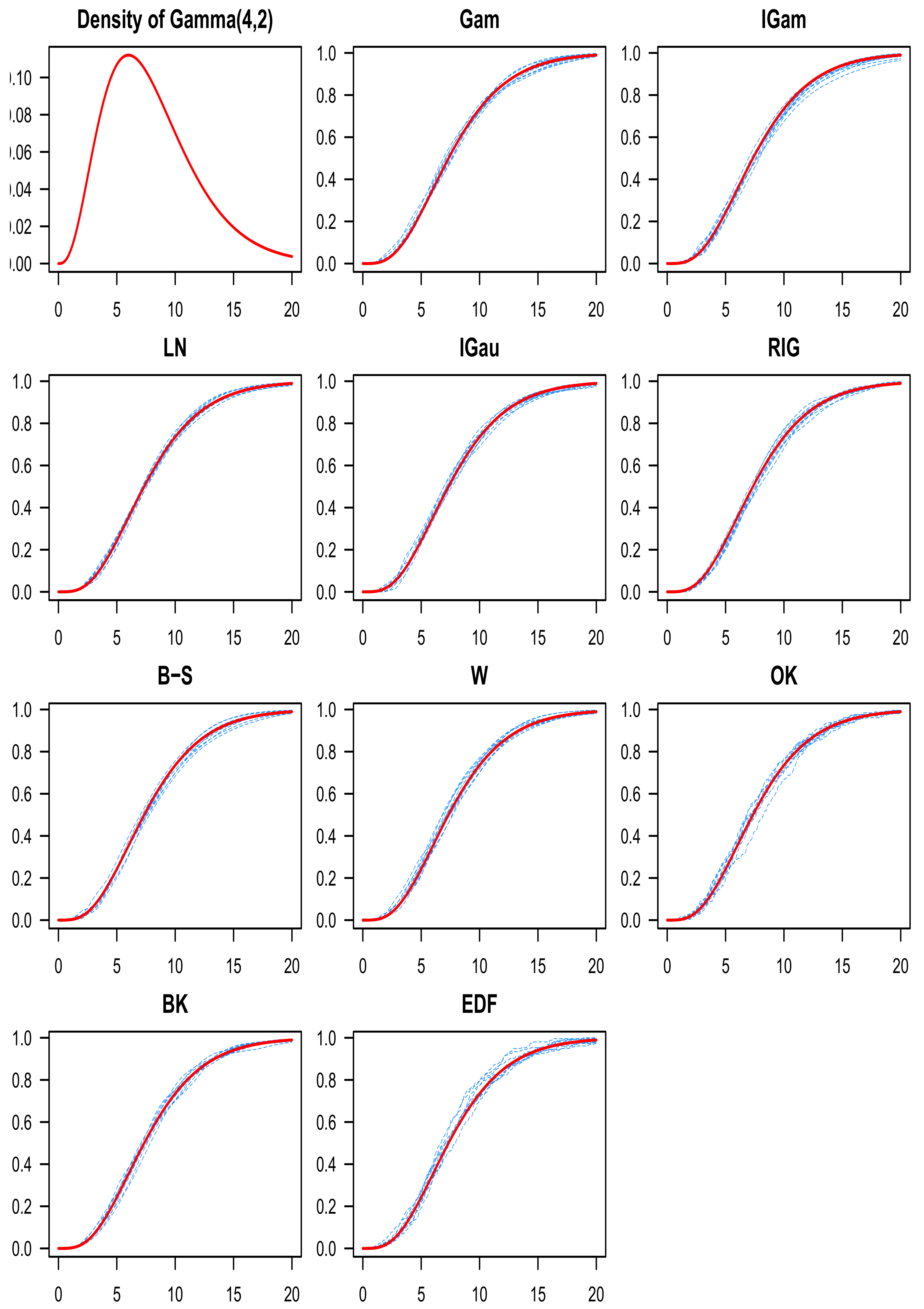
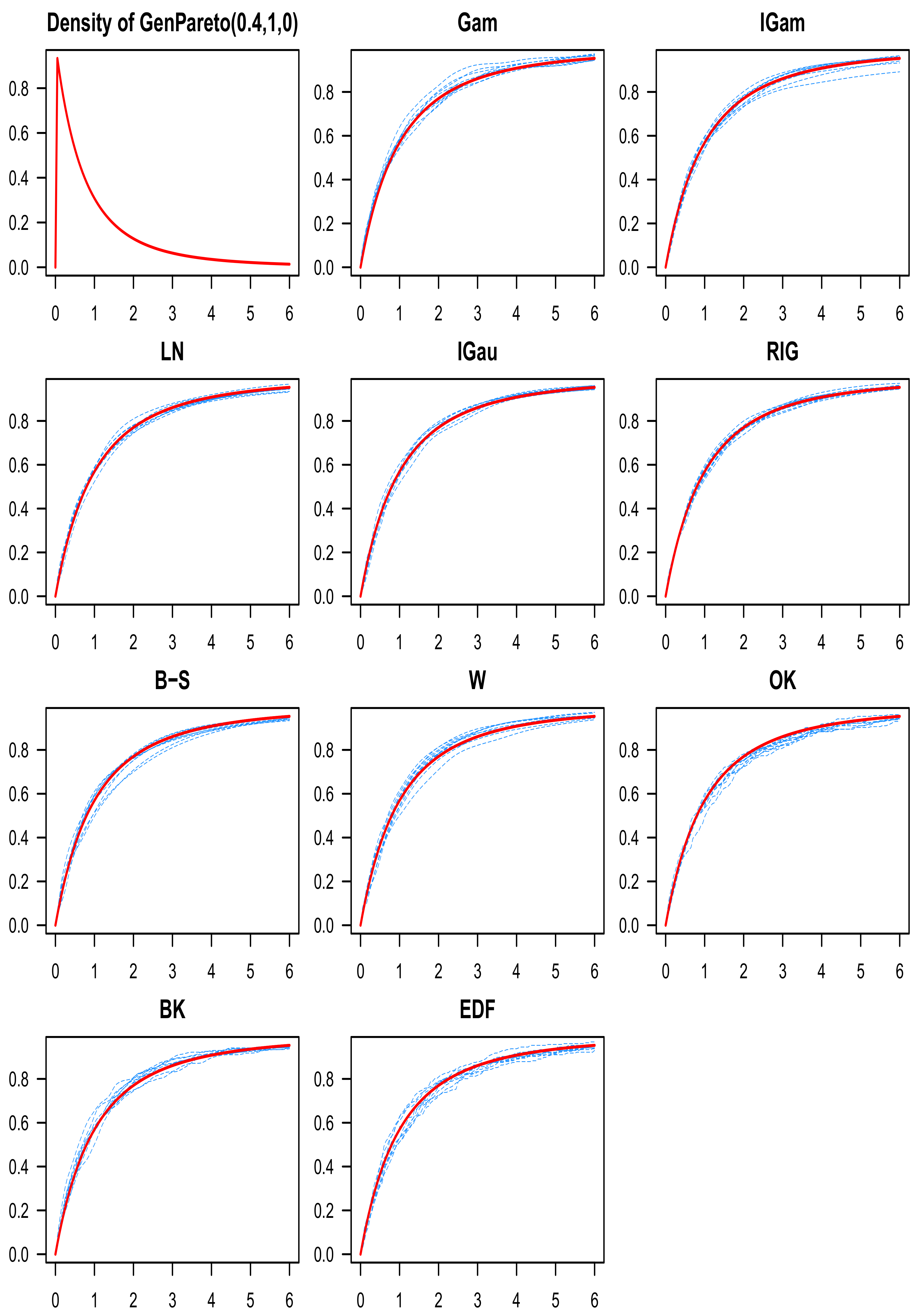
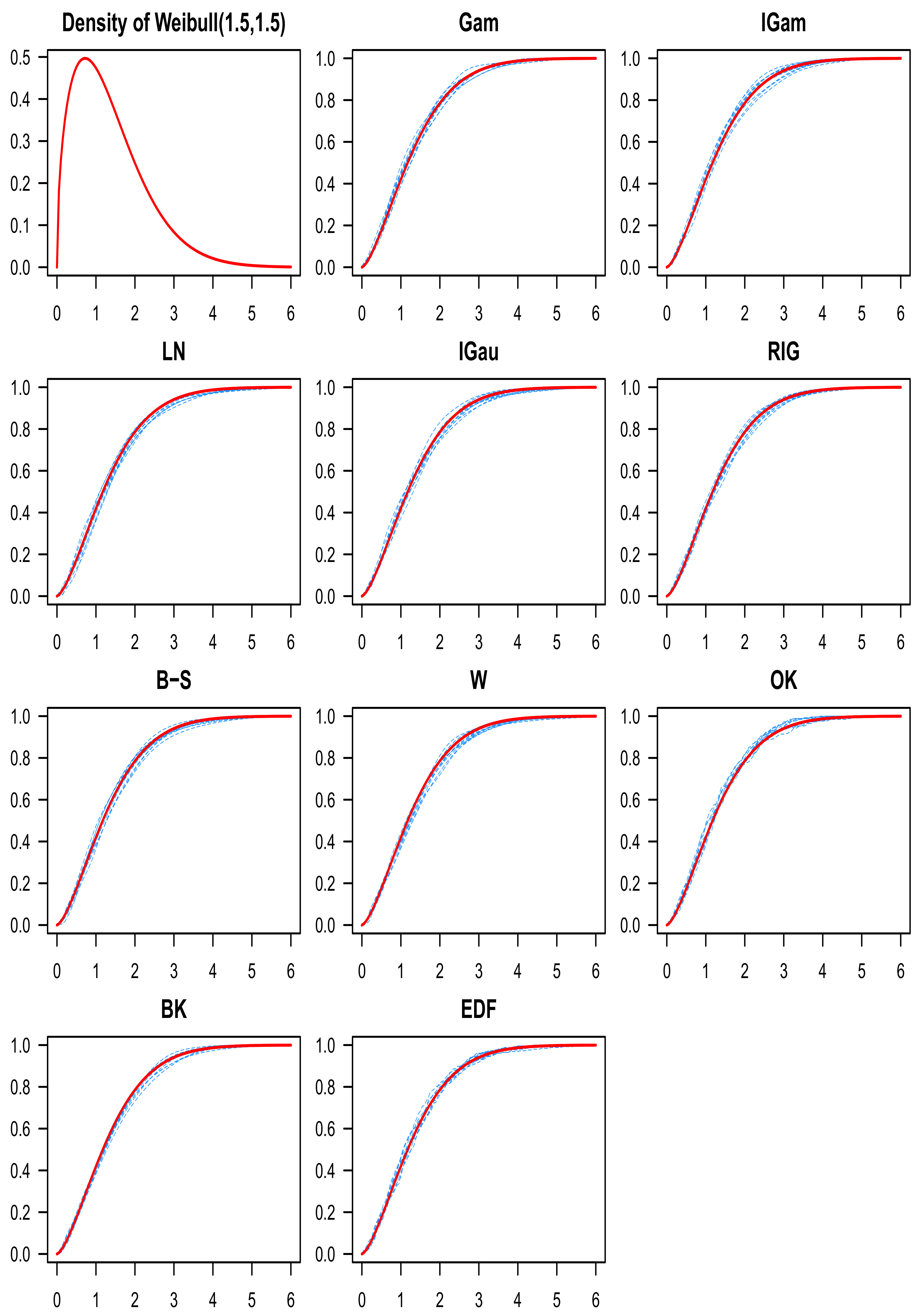
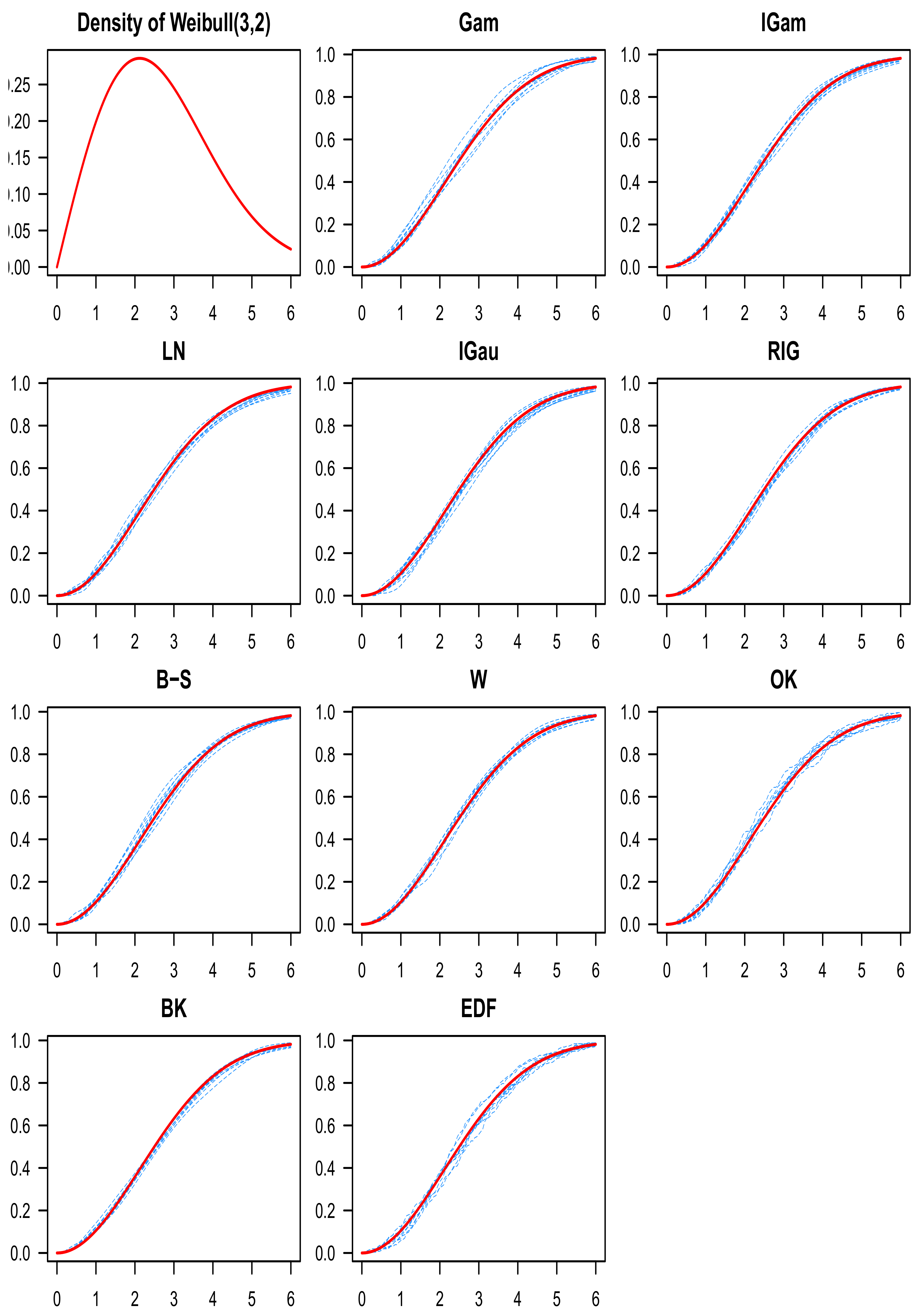
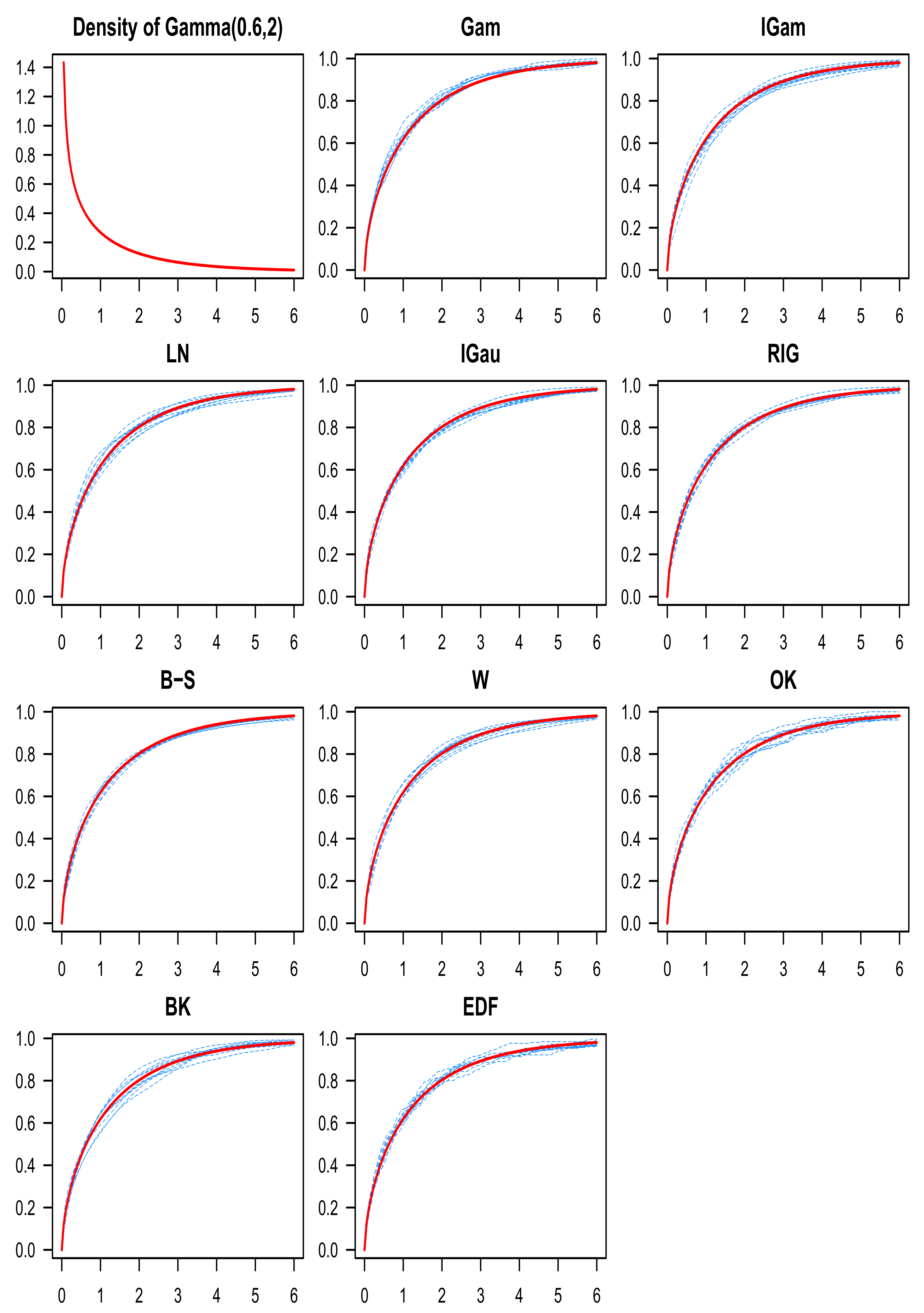
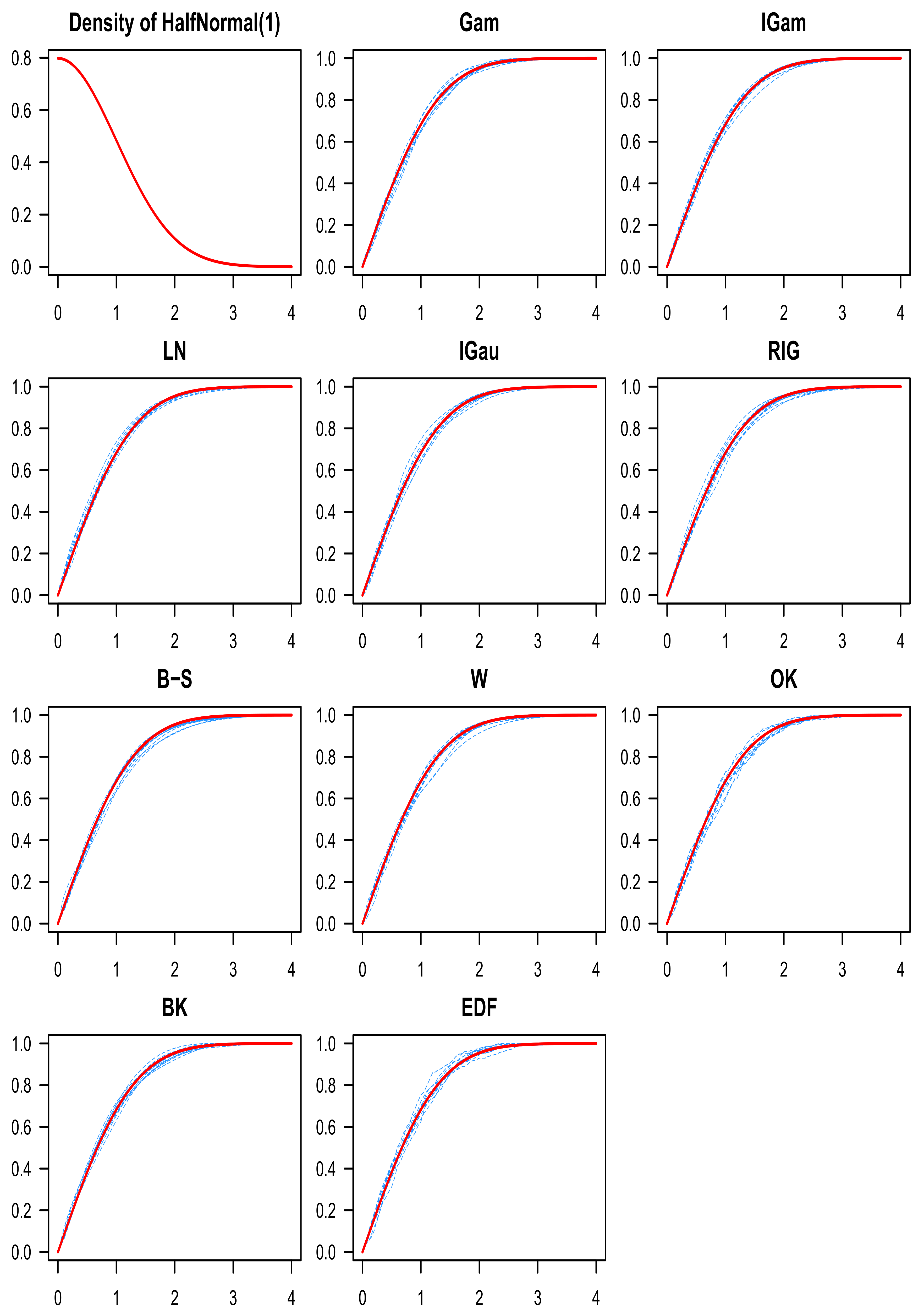
In this section, we find the asymptotic properties of the reciprocal inverse Gaussian (RIG) kernel estimator defined in (5).

Lemma 5

(Bias and variance). For any given $x\in (0,\infty )$,

$$\mathbb{B}\mathrm{ias}[{\widehat{F}}_{n,b}^{\mathrm{RIG}}\left(x\right)]:=\mathbb{E}[{\widehat{F}}_{n,b}^{\mathrm{IGau}}\left(x\right)]-F\left(x\right)=b·\frac{x^2}{2}{f}^{\prime }\left(x\right)+{\mathrm{o}}_x\left(b\right),$$

(59)

$$\begin{array}{cc}\hfill \mathbb{V}\mathrm{ar}\left({\widehat{F}}_{n,b}^{\mathrm{RIG}}\left(x\right)\right)& =n^{-1}F\left(x\right)(1-F\left(x\right))-n^{-1}{b}^{1/2}·\frac{f\left(x\right)}{2}\left[\underset{b\to 0}{lim}{b}^{-1/2}\mathbb{E}[|T_1-T_2|]\right]\hfill \\ \hfill & +{\mathcal{O}}_x\left(n^{-1}b\right),\hfill \end{array}$$

(60)

where $T_1,T_2\stackrel{\mathrm{i}.\mathrm{i}.\mathrm{d}.}{\sim }\mathrm{RIG}(x,b^{-1}x)$.

Corollary 5

(Mean squared error). For any given $x\in (0,\infty )$,

$$\begin{array}{cc}\hfill \mathrm{MSE}\left({\widehat{F}}_{n,b}^{\mathrm{RIG}}\left(x\right)\right)& =\mathbb{V}\mathrm{ar}\left({\widehat{F}}_{n,b}^{\mathrm{RIG}}\left(x\right)\right)+{\left(\mathbb{B}\mathrm{ias}[{\widehat{F}}_{n,b}^{\mathrm{RIG}}\left(x\right)]\right)}^2\hfill \\ \hfill & =n^{-1}F\left(x\right)(1-F\left(x\right))-n^{-1}{b}^{1/2}·\frac{f\left(x\right)}{2}\left[\underset{b\to 0}{lim}{b}^{-1/2}\mathbb{E}[|T_1-T_2|]\right]\hfill \\ \hfill & +b^2·\frac{1}{4}{x}^4{\left(f^{\prime }\left(x\right)\right)}^2+{\mathcal{O}}_x\left(n^{-1}b\right)+{\mathrm{o}}_x\left(b^2\right),\hfill \end{array}$$

(61)

where $T_1,T_2\stackrel{\mathrm{i}.\mathrm{i}.\mathrm{d}.}{\sim }\mathrm{RIG}(x^{-1}{(1-b)}^{-1},x^{-1}{b}^{-1})$. The quantity ${lim}_{b\to 0}{b}^{-1/2}\mathbb{E}[|T_1-T_2|]$ needs to be approximated numerically. In particular, if $f\left(x\right)\left[{lim}_{b\to 0}{b}^{-1/2}\mathbb{E}[|T_1-T_2|]\right]·f^{\prime }\left(x\right)\ne 0$, the asymptotically optimal choice of b, with respect to $\mathrm{MSE}$, is

$$b_{\mathrm{opt}}=n^{-2/3}{\left[\frac{4·\frac{1}{4}{x}^4{\left(f^{\prime }\left(x\right)\right)}^2}{\frac{f\left(x\right)}{2}{lim}_{b\to 0}{b}^{-1/2}\mathbb{E}[|T_1-T_2|]}\right]}^{-2/3}$$

(62)

with

$$\begin{array}{cc}\hfill \mathrm{MSE}\left({\widehat{F}}_{n,b_{\mathrm{opt}}}^{\mathrm{RIG}}\left(x\right)\right)& =n^{-1}F\left(x\right)(1-F\left(x\right))\hfill \\ \hfill & -n^{-4/3}\frac{3}{4}{\left[\frac{{\left(\frac{f\left(x\right)}{2}{lim}_{b\to 0}{b}^{-1/2}\mathbb{E}[|T_1-T_2|]\right)}^4}{4·\frac{1}{4}{x}^4{\left(f^{\prime }\left(x\right)\right)}^2}\right]}^{1/3}+{\mathrm{o}}_x\left(n^{-4/3}\right).\hfill \end{array}$$

(63)

Proposition 9

(Mean integrated squared error). Assuming that the target density $f=F^{\prime }$ satisfies

$${\int }_0^{\infty }f\left(x\right)\left[\underset{b\to 0}{lim}{b}^{-1/2}\mathbb{E}[|T_1-T_2|]\right]\mathrm{d}x<\infty and{\int }_0^{\infty }{x}^4{\left(f^{\prime }\left(x\right)\right)}^2\mathrm{d}x<\infty ,$$

(64)

where $T_1,T_2\stackrel{\mathrm{i}.\mathrm{i}.\mathrm{d}.}{\sim }\mathrm{RIG}(x^{-1}{(1-b)}^{-1},x^{-1}{b}^{-1})$, then we have

$$\begin{array}{cc}\hfill \mathrm{MISE}\left({\widehat{F}}_{n,b}^{\mathrm{RIG}}\left(x\right)\right)& ={\int }_0^{\infty }\mathbb{V}\mathrm{ar}\left({\widehat{F}}_{n,b}^{\mathrm{RIG}}\left(x\right)\right)\mathrm{d}x+{\int }_0^{\infty }{\left(\mathbb{B}\mathrm{ias}[{\widehat{F}}_{n,b}^{\mathrm{RIG}}\left(x\right)]\right)}^2\mathrm{d}x\hfill \\ \hfill & =n^{-1}{\int }_0^{\infty }F\left(x\right)(1-F\left(x\right))\mathrm{d}x\hfill \\ \hfill & -n^{-1}{b}^{1/2}{\int }_0^{\infty }\frac{f\left(x\right)}{2}\left[\underset{b\to 0}{lim}{b}^{-1/2}\mathbb{E}[|T_1-T_2|]\right]\mathrm{d}x\hfill \\ \hfill & +b^2{\int }_0^{\infty }\frac{x^4}{4}{\left(f^{\prime }\left(x\right)\right)}^2\mathrm{d}x+\mathrm{o}\left(n^{-1}{b}^{1/2}\right)+\mathrm{o}\left(b^2\right).\hfill \end{array}$$

(65)

The quantity ${lim}_{b\to 0}{b}^{-1/2}\mathbb{E}[|T_1-T_2|]$ needs to be approximated numerically. In particular, if ${\int }_0^{\infty }{x}^4{\left(f^{\prime }\left(x\right)\right)}^2\mathrm{d}x>0$, the asymptotically optimal choice of b, with respect to $\mathrm{MISE}$, is

$$b_{\mathrm{opt}}=n^{-2/3}{\left[\frac{4{\int }_0^{\infty }\frac{1}{4}{x}^4{\left(f^{\prime }\left(x\right)\right)}^2\mathrm{d}x}{{\int }_0^{\infty }\frac{f\left(x\right)}{2}{lim}_{b\to 0}{b}^{-1/2}\mathbb{E}[|T_1-T_2|]\mathrm{d}x}\right]}^{-2/3}$$

(66)

with

$$\begin{array}{cc}\hfill \mathrm{MISE}\left({\widehat{F}}_{n,b_{\mathrm{opt}}}^{\mathrm{RIG}}\left(x\right)\right)& =n^{-1}{\int }_0^{\infty }F\left(x\right)(1-F\left(x\right))\mathrm{d}x\hfill \\ \hfill & -n^{-4/3}\frac{3}{4}{\left[\frac{{\left({\int }_0^{\infty }\frac{f\left(x\right)}{2}{lim}_{b\to 0}{b}^{-1/2}\mathbb{E}[|T_1-T_2|]\mathrm{d}x\right)}^4}{4{\int }_0^{\infty }\frac{1}{4}{x}^4{\left(f^{\prime }\left(x\right)\right)}^2\mathrm{d}x}\right]}^{1/3}\hfill \\ \hfill & +\mathrm{o}\left(n^{-4/3}\right).\hfill \end{array}$$

(67)

Proposition 10

(Asymptotic normality). For any $x>0$ such that $0<F\left(x\right)<1$, we have the following convergence in distribution:

$$n^{1/2}({\widehat{F}}_{n,b}^{\mathrm{RIG}}\left(x\right)-\mathbb{E}[{\widehat{F}}_{n,b}^{\mathrm{IGau}}\left(x\right)])\stackrel{\mathcal{D}}{⟶}\mathcal{N}(0,{\sigma }^2\left(x\right)),asb\to 0,n\to \infty ,$$

(68)

where ${\sigma }^2\left(x\right)=F\left(x\right)(1-F\left(x\right))$. In particular, Lemma 5 implies

$$\begin{array}{cccc}& n^{1/2}({\widehat{F}}_{n,b}^{\mathrm{RIG}}\left(x\right)-F\left(x\right))\stackrel{\mathcal{D}}{⟶}\mathcal{N}(0,{\sigma }^2\left(x\right)),\hfill & & if{n}^{1/2}b\to 0,\hfill \end{array}$$

(69)

$$\begin{array}{cccc}& n^{1/2}({\widehat{F}}_{n,b}^{\mathrm{RIG}}\left(x\right)-F\left(x\right))\stackrel{\mathcal{D}}{⟶}\mathcal{N}(\lambda ·\frac{x^2}{2}{f}^{\prime }\left(x\right),{\sigma }^2\left(x\right)),\hfill & & if{n}^{1/2}b\to \lambda ,\hfill \end{array}$$

(70)

for any constant $\lambda >0$.

8. Numerical Study

As in [41], we generated $M=1000$ samples of size $n=256$ and $n=1000$ from eight target distributions:

• Burr $(1,3,1)$, with the following parametrization for the density function:

  $$\begin{array}{c}{f}_1\left(x\right|\lambda ,c,k):=\frac{ck}{\lambda }{\left(\frac{x}{\lambda }\right)}^{c-1}{\left[1+{\left(\frac{x}{\lambda }\right)}^c\right]}^{-k-1}{𝟙}_{(0,\infty )}\left(x\right),\lambda ,c,k>0;\hfill \end{array}$$

  (71)
• Gamma $(0.6,2)$, with the following parametrization for the density function:

  $$\begin{array}{c}{f}_2\left(x\right|\alpha ,\theta ):=\frac{x^{\alpha -1}exp(-\frac{x}{\theta })}{{\theta }^{\alpha }\Gamma \left(\alpha \right)}{𝟙}_{(0,\infty )}\left(x\right),\alpha ,\theta >0;\hfill \end{array}$$

  (72)
• Gamma $(4,2)$, with the following parametrization for the density function:

  $$\begin{array}{c}{f}_3\left(x\right|\alpha ,\theta ):=\frac{x^{\alpha -1}exp(-\frac{x}{\theta })}{{\theta }^{\alpha }\Gamma \left(\alpha \right)}{𝟙}_{(0,\infty )}\left(x\right),\alpha ,\theta >0;\hfill \end{array}$$

  (73)
• GeneralizedPareto $(0.4,1,0)$, with the following parametrization for the density function:

  $$\begin{array}{c}{f}_4\left(x\right|\xi ,\sigma ,\mu ):=\frac{1}{\sigma }{\left[1+\xi \left(\frac{x-\mu }{\sigma }\right)\right]}^{-\frac{1}{\xi }-1}{𝟙}_{(\mu ,\infty )}\left(x\right),\xi ,\sigma >0,\mu \in \mathbb{R};\hfill \end{array}$$

  (74)
• HalfNormal $\left(1\right)$, with the following parametrization for the density function:

  $$\begin{array}{c}{f}_5\left(x\right|\sigma ):=\sqrt{\frac{2}{\pi {\sigma }^2}}exp\left(-\frac{x^2}{2{\sigma }^2}\right){𝟙}_{(0,\infty )}\left(x\right),\sigma >0;\hfill \end{array}$$

  (75)
• LogNormal $(0,0.75)$, with the following parametrization for the density function:

  $$\begin{array}{c}{f}_6\left(x\right|\mu ,\sigma ):=\frac{1}{x\sqrt{2\pi {\sigma }^2}}exp\left(-\frac{{(logx-\mu )}^2}{2{\sigma }^2}\right){𝟙}_{(0,\infty )}\left(x\right),\mu \in \mathbb{R},\sigma >0;\hfill \end{array}$$

  (76)
• Weibull $(1.5,1.5)$, with the following parametrization for the density function:

  $$\begin{array}{c}{f}_7\left(x\right|\lambda ,k):=\frac{k}{\lambda }{\left(\frac{x}{\lambda }\right)}^{k-1}exp\left(-{\left(\frac{x}{\lambda }\right)}^k\right){𝟙}_{(0,\infty )}\left(x\right),\lambda ,k>0;\hfill \end{array}$$

  (77)
• Weibull $(3,2)$, with the following parametrization for the density function:

  $$\begin{array}{c}{f}_8\left(x\right|\lambda ,k):=\frac{k}{\lambda }{\left(\frac{x}{\lambda }\right)}^{k-1}exp\left(-{\left(\frac{x}{\lambda }\right)}^k\right){𝟙}_{(0,\infty )}\left(x\right),\lambda ,k>0.\hfill \end{array}$$

  (78)

For each of the eight target distributions ($i=1,2,\dots ,8$), each of the ten estimators ($j=1,2,\dots ,10$), each sample size ($n=256,1000$), and each sample ($k=1,2,\dots ,M$), we calculated the integrated squared errors

$${\mathrm{ISE}}_{i,j,n}^{\left(k\right)}:={\int }_0^{\infty }{({\widehat{F}}_{j,n}^{\left(k\right)}\left(x\right)-F_i\left(x\right))}^2\mathrm{d}x,$$

(79)

where

• ${\widehat{F}}_{1,n}^{\left(k\right)}$ denotes the estimator ${\widehat{F}}_{n,b_{\mathrm{opt}}}^{\mathrm{Gam}}$ from (1) applied to the k-th sample;
• ${\widehat{F}}_{2,n}^{\left(k\right)}$ denotes the estimator ${\widehat{F}}_{n,b_{\mathrm{opt}}}^{\mathrm{IGam}}$ from (2) applied to the k-th sample;
• ${\widehat{F}}_{3,n}^{\left(k\right)}$ denotes the estimator ${\widehat{F}}_{n,b_{\mathrm{opt}}}^{\mathrm{LN}}$ from (3) applied to the k-th sample;
• ${\widehat{F}}_{4,n}^{\left(k\right)}$ denotes the estimator ${\widehat{F}}_{n,b_{\mathrm{opt}}}^{\mathrm{IGau}}$ from (4) applied to the k-th sample;
• ${\widehat{F}}_{5,n}^{\left(k\right)}$ denotes the estimator ${\widehat{F}}_{n,b_{\mathrm{opt}}}^{\mathrm{RIG}}$ from (5) applied to the k-th sample;
• ${\widehat{F}}_{6,n}^{\left(k\right)}$ denotes the estimator ${\widehat{F}}_{n,b_{\mathrm{opt}}}^{\mathrm{B}-\mathrm{S}}$ from (6) applied to the k-th sample;
• ${\widehat{F}}_{7,n}^{\left(k\right)}$ denotes the estimator ${\widehat{F}}_{n,b_{\mathrm{opt}}}^{\mathrm{W}}$ from (7) applied to the k-th sample;
  (for ${\widehat{F}}_{1,n}^{\left(k\right)}$ to ${\widehat{F}}_{7,n}^{\left(k\right)}$, $b_{\mathrm{opt}}$ is optimal with respect to the MISE (see (18), (30), (42), (54) and (66)) and approximated under the assumption that the target distribution is $\mathrm{Gamma}({\widehat{\alpha }}_n^{\left(k\right)},{\widehat{\theta }}_n^{\left(k\right)})$, where ${\widehat{\alpha }}_n^{\left(k\right)}$ and ${\widehat{\theta }}_n^{\left(k\right)}$ are the maximum likelihood estimates for the k-th sample) and
• ${\widehat{F}}_{8,n}^{\left(k\right)}\left(x\right):=\frac{1}{n}{\sum }_{\ell =1}^n\mathrm{Epa}\left(\frac{x-X_{\ell }^{\left(k\right)}}{b_{\mathrm{LNO}}}\right)$, where
  • $\mathrm{Epa}\left(u\right)=\left(\frac{1}{2}+\frac{3u}{4}-\frac{u^3}{4}\right)·{𝟙}_{(-1,1)}\left(u\right)+{𝟙}_{[1,\infty )}\left(u\right)$ denotes the c.d.f. of the Epanechnikov kernel;
  • $b_{\mathrm{LNO}}$ is selected by minimizing the Leave-None-Out criterion from page 197 in [61];
• ${\widehat{F}}_{9,n}^{\left(k\right)}\left(x\right):=\frac{1}{n}{\sum }_{\ell =1}^n\left\{\mathrm{Epa}\left(\frac{x-X_{\ell }^{\left(k\right)}}{b_{\mathrm{CV}}}\right){𝟙}_{[b_{\mathrm{CV}},\infty )}\left(x\right)+\mathrm{Epa}\left(\frac{x-X_{\ell }^{\left(k\right)}}{x}\right){𝟙}_{(0,b_{\mathrm{CV}})}\left(x\right)\right\}$ is the boundary modified kernel estimator from Example 2.3 in [57], where
  • $\mathrm{Epa}\left(u\right)=\left(\frac{1}{2}+\frac{3u}{4}-\frac{u^3}{4}\right)·{𝟙}_{(-1,1)}\left(u\right)+{𝟙}_{[1,\infty )}\left(u\right)$ denotes the c.d.f. of the Epanechnikov kernel;
  • $b_{\mathrm{CV}}$ is selected by minimizing the Cross-Validation criterion from page 180 in [57];
• ${\widehat{F}}_{10,n}^{\left(k\right)}\left(x\right):=\frac{1}{n}{\sum }_{\ell =1}^n{𝟙}_{\{X_{\ell }^{\left(k\right)}\le x\}}$ is the empirical c.d.f. applied to the k-th sample.

Everywhere in our R code, we approximated the integrals on $(0,\infty )$ using the integral function from the R package pracma (the base function integrate had serious precision issues). Table 1 below shows the mean and standard deviation of the $\mathrm{ISE}$’s, i.e.,

$$\frac{1}{M}\sum _{k=1}^M{\mathrm{ISE}}_{i,j,n}^{\left(k\right)}\mathrm{and}\sqrt{\frac{1}{M-1}\sum _{k=1}^M{\left({\mathrm{ISE}}_{i,j,n}^{\left(k\right)}-\frac{1}{M}\sum _{k^{\prime }=1}^M{\mathrm{ISE}}_{i,j,n}^{\left(k^{\prime }\right)}\right)}^2},$$

(80)

for the eight target distributions ($i=1,2,\dots ,8$), the ten estimators ($j=1,2,\dots ,10$) and the two sample sizes ($n=256,1000$). All the values presented in the table have been multiplied by ${10}^4$. In Table 2, we computed, for each target distribution and each sample size, the difference between the $\mathrm{ISE}$ means and the lowest $\mathrm{ISE}$ mean for the corresponding target distribution and sample size (i.e., the $\mathrm{ISE}$ means minus the $\mathrm{ISE}$ mean of the best estimator on the corresponding line). The totals of those differences are also calculated for each sample size on the two “total” lines. Figure 1 gives a better idea of the target distribution of $\mathrm{ISE}$’s by displaying the boxplot of the $\mathrm{ISE}$’s for every target distribution and every estimator, when the sample size is $n=1000$. Finally, Figure 2, Figure 3, Figure 4, Figure 5, Figure 6, Figure 7, Figure 8 and Figure 9 (one figure for each of the eight target distributions) show a collection of ten c.d.f. estimates from each of the ten estimators when the sample size is 256.

Here are the results, which we discuss briefly in Section 9:

Figure 1. Boxplots of the ${\mathrm{ISE}}_{i,j,n}^{\left(k\right)},k=1,2,\dots ,M$, for the eight target distributions and the ten estimators, when the sample size is n = 1000. (a) Burr(1, 3, 1). (b) Gamma(0.6, 2). (c) Gamma(4, 2). (d) GeneralizedPareto(0.4, 1, 0). (e) HalfNormal(1). (f) LogNormal(0, 0.75). (g) Weibull(1.5, 1.5). (h) Weibull(3, 2).

Figure 1. Boxplots of the ${\mathrm{ISE}}_{i,j,n}^{\left(k\right)},k=1,2,\dots ,M$, for the eight target distributions and the ten estimators, when the sample size is n = 1000. (a) Burr(1, 3, 1). (b) Gamma(0.6, 2). (c) Gamma(4, 2). (d) GeneralizedPareto(0.4, 1, 0). (e) HalfNormal(1). (f) LogNormal(0, 0.75). (g) Weibull(1.5, 1.5). (h) Weibull(3, 2).

Table 1. The mean and standard deviation of the ${\mathrm{ISE}}_{i,j,n}^{\left(k\right)},k=1,2,\dots ,M$, for the eight target distributions ($i=1,2,\dots ,8$), the ten estimators ($j=1,2,\dots ,10$) and the two sample sizes ($n=256,1000$). All the values presented in the table have been multiplied by ${10}^4$. The ordinary kernel estimator ${\widehat{F}}_8$ is denoted by $\mathrm{OK}$, the boundary kernel estimator ${\widehat{F}}_9$ is denoted by $\mathrm{BK}$, and the empirical c.d.f. ${\widehat{F}}_{10}$ is denoted by $\mathrm{EDF}$. For each line in the table, the lowest $\mathrm{ISE}$ means are highlighted in cyan.

$\times {10}^{-4}$	i	Gam ($\mathit{i}=1$)		IGam ($\mathit{i}=2$)		LN ($\mathit{i}=3$)		IGau ($\mathit{i}=4$)		RIG ($\mathit{i}=5$)		B-S ($\mathit{i}=6$)		W ($\mathit{i}=7$)		OK ($\mathit{i}=8$)		BK ($\mathit{i}=9$)		EDF ($\mathit{i}=10$)
$\mathit{n}$	$\mathit{j}$	Mean	Std.	Mean	Std.	Mean	Std.	Mean	Std.	Mean	Std.	Mean	Std.	Mean	Std.	Mean	Std.	Mean	Std.	Mean	Std.
256	1	1.39	1.27	1.37	1.34	1.31	1.26	1.37	1.32	1.37	1.32	1.31	1.26	1.37	1.32	1.54	1.43	1.47	1.34	1.54	1.44
	2	2.59	2.36	2.50	2.53	2.36	2.42	2.49	2.46	2.49	2.47	2.36	2.42	2.50	2.51	2.76	2.44	2.67	2.57	2.76	2.45
	3	6.70	6.28	6.77	6.58	6.62	6.28	6.69	6.45	6.69	6.45	6.62	6.28	6.74	6.54	7.44	7.01	6.70	6.39	7.44	7.00
	4	3.74	3.14	3.60	3.27	3.36	3.15	3.61	3.20	3.61	3.21	3.36	3.14	3.60	3.26	3.96	3.24	3.80	3.27	3.97	3.24
	5	1.14	1.10	1.18	1.13	1.18	1.07	1.17	1.13	1.17	1.13	1.18	1.07	1.17	1.12	1.26	1.19	1.10	1.14	1.26	1.19
	6	1.93	1.83	1.91	1.89	1.81	1.80	1.91	1.87	1.91	1.87	1.81	1.80	1.91	1.88	2.13	1.94	2.05	1.93	2.13	1.95
	7	1.75	1.82	1.77	1.99	1.68	1.83	1.76	1.96	1.76	1.96	1.68	1.83	1.76	1.95	1.95	1.93	1.73	2.04	1.95	1.92
	8	2.69	2.71	2.75	2.78	2.81	2.66	2.67	2.71	2.67	2.71	2.81	2.66	2.75	2.75	3.02	2.88	2.56	2.59	3.03	2.88
1000	1	0.40	0.36	0.39	0.36	0.38	0.35	0.39	0.36	0.39	0.36	0.38	0.35	0.39	0.36	0.43	0.39	0.41	0.36	0.43	0.39
	2	0.72	0.70	0.70	0.69	0.67	0.67	0.70	0.69	0.70	0.69	0.67	0.67	0.70	0.69	0.75	0.71	0.73	0.72	0.75	0.71
	3	2.01	2.09	2.05	2.22	2.02	2.16	2.04	2.15	2.04	2.15	2.02	2.16	2.05	2.20	2.23	2.29	1.99	2.09	2.23	2.30
	4	0.99	0.79	0.97	0.82	0.93	0.80	0.97	0.81	0.97	0.81	0.93	0.80	0.97	0.82	1.03	0.82	1.00	0.82	1.03	0.83
	5	0.31	0.31	0.31	0.31	0.31	0.30	0.31	0.31	0.31	0.31	0.31	0.30	0.31	0.31	0.33	0.32	0.30	0.32	0.33	0.32
	6	0.47	0.43	0.47	0.43	0.46	0.42	0.47	0.43	0.47	0.43	0.46	0.42	0.47	0.43	0.50	0.45	0.49	0.43	0.50	0.45
	7	0.46	0.46	0.46	0.48	0.44	0.45	0.46	0.48	0.46	0.48	0.44	0.45	0.46	0.48	0.49	0.50	0.46	0.48	0.49	0.50
	8	0.72	0.74	0.74	0.75	0.75	0.74	0.73	0.75	0.73	0.75	0.75	0.74	0.74	0.75	0.78	0.80	0.70	0.72	0.78	0.81

Table 1. The mean and standard deviation of the ${\mathrm{ISE}}_{i,j,n}^{\left(k\right)},k=1,2,\dots ,M$, for the eight target distributions ($i=1,2,\dots ,8$), the ten estimators ($j=1,2,\dots ,10$) and the two sample sizes ($n=256,1000$). All the values presented in the table have been multiplied by ${10}^4$. The ordinary kernel estimator ${\widehat{F}}_8$ is denoted by $\mathrm{OK}$, the boundary kernel estimator ${\widehat{F}}_9$ is denoted by $\mathrm{BK}$, and the empirical c.d.f. ${\widehat{F}}_{10}$ is denoted by $\mathrm{EDF}$. For each line in the table, the lowest $\mathrm{ISE}$ means are highlighted in cyan.

$\times {10}^{-4}$	i	Gam ($\mathit{i}=1$)		IGam ($\mathit{i}=2$)		LN ($\mathit{i}=3$)		IGau ($\mathit{i}=4$)		RIG ($\mathit{i}=5$)		B-S ($\mathit{i}=6$)		W ($\mathit{i}=7$)		OK ($\mathit{i}=8$)		BK ($\mathit{i}=9$)		EDF ($\mathit{i}=10$)
$\mathit{n}$	$\mathit{j}$	Mean	Std.	Mean	Std.	Mean	Std.	Mean	Std.	Mean	Std.	Mean	Std.	Mean	Std.	Mean	Std.	Mean	Std.	Mean	Std.
256	1	1.39	1.27	1.37	1.34	1.31	1.26	1.37	1.32	1.37	1.32	1.31	1.26	1.37	1.32	1.54	1.43	1.47	1.34	1.54	1.44
	2	2.59	2.36	2.50	2.53	2.36	2.42	2.49	2.46	2.49	2.47	2.36	2.42	2.50	2.51	2.76	2.44	2.67	2.57	2.76	2.45
	3	6.70	6.28	6.77	6.58	6.62	6.28	6.69	6.45	6.69	6.45	6.62	6.28	6.74	6.54	7.44	7.01	6.70	6.39	7.44	7.00
	4	3.74	3.14	3.60	3.27	3.36	3.15	3.61	3.20	3.61	3.21	3.36	3.14	3.60	3.26	3.96	3.24	3.80	3.27	3.97	3.24
	5	1.14	1.10	1.18	1.13	1.18	1.07	1.17	1.13	1.17	1.13	1.18	1.07	1.17	1.12	1.26	1.19	1.10	1.14	1.26	1.19
	6	1.93	1.83	1.91	1.89	1.81	1.80	1.91	1.87	1.91	1.87	1.81	1.80	1.91	1.88	2.13	1.94	2.05	1.93	2.13	1.95
	7	1.75	1.82	1.77	1.99	1.68	1.83	1.76	1.96	1.76	1.96	1.68	1.83	1.76	1.95	1.95	1.93	1.73	2.04	1.95	1.92
	8	2.69	2.71	2.75	2.78	2.81	2.66	2.67	2.71	2.67	2.71	2.81	2.66	2.75	2.75	3.02	2.88	2.56	2.59	3.03	2.88
1000	1	0.40	0.36	0.39	0.36	0.38	0.35	0.39	0.36	0.39	0.36	0.38	0.35	0.39	0.36	0.43	0.39	0.41	0.36	0.43	0.39
	2	0.72	0.70	0.70	0.69	0.67	0.67	0.70	0.69	0.70	0.69	0.67	0.67	0.70	0.69	0.75	0.71	0.73	0.72	0.75	0.71
	3	2.01	2.09	2.05	2.22	2.02	2.16	2.04	2.15	2.04	2.15	2.02	2.16	2.05	2.20	2.23	2.29	1.99	2.09	2.23	2.30
	4	0.99	0.79	0.97	0.82	0.93	0.80	0.97	0.81	0.97	0.81	0.93	0.80	0.97	0.82	1.03	0.82	1.00	0.82	1.03	0.83
	5	0.31	0.31	0.31	0.31	0.31	0.30	0.31	0.31	0.31	0.31	0.31	0.30	0.31	0.31	0.33	0.32	0.30	0.32	0.33	0.32
	6	0.47	0.43	0.47	0.43	0.46	0.42	0.47	0.43	0.47	0.43	0.46	0.42	0.47	0.43	0.50	0.45	0.49	0.43	0.50	0.45
	7	0.46	0.46	0.46	0.48	0.44	0.45	0.46	0.48	0.46	0.48	0.44	0.45	0.46	0.48	0.49	0.50	0.46	0.48	0.49	0.50
	8	0.72	0.74	0.74	0.75	0.75	0.74	0.73	0.75	0.73	0.75	0.75	0.74	0.74	0.75	0.78	0.80	0.70	0.72	0.78	0.81

Table 2. For each of the eight target distributions ($i=1,2,\dots ,8$) and each of the two sample sizes ($n=256,1000$), a cell represents the mean of the ${\mathrm{ISE}}_{i,j,n}^{\left(k\right)},k=1,2,\dots ,M$, minus the lowest $\mathrm{ISE}$ mean for that line (i.e., minus the $\mathrm{ISE}$ mean of the best estimator for that specific target distribution and sample size). For each estimator ($j=1,2,\dots ,10$) and each sample size, the total of those differences to the best $\mathrm{ISE}$ means is calculated on the line called “total”. For each sample size, the lowest totals are highlighted in cyan.

$\times {10}^{-4}$	i	Gam ($\mathit{i}=1$)	IGam ($\mathit{i}=2$)	LN ($\mathit{i}=3$)	IGau ($\mathit{i}=4$)	RIG ($\mathit{i}=5$)	B-S ($\mathit{i}=6$)	W ($\mathit{i}=7$)	OK ($\mathit{i}=8$)	BK ($\mathit{i}=9$)	EDF ($\mathit{i}=10$)
$\mathit{n}$	$\mathit{j}$	Diff. with	Diff. with	Diff. with	Diff. with	Diff. with	Diff. with	Diff. with	Diff. with	Diff. with	Diff. with
		Lowest	Lowest	Lowest	Lowest	Lowest	Lowest	Lowest	Lowest	Lowest	Lowest
		Mean	Mean	Mean	Mean	Mean	Mean	Mean	Mean	Mean	Mean
256	1	0.08	0.06	0.00	0.06	0.06	0.00	0.06	0.23	0.16	0.23
	2	0.23	0.14	0.00	0.14	0.13	0.00	0.14	0.40	0.32	0.40
	3	0.08	0.15	0.01	0.08	0.07	0.00	0.12	0.82	0.09	0.82
	4	0.38	0.24	0.00	0.25	0.24	0.00	0.23	0.60	0.43	0.60
	5	0.05	0.08	0.09	0.07	0.07	0.08	0.08	0.16	0.00	0.17
	6	0.12	0.10	0.00	0.10	0.10	0.00	0.10	0.32	0.24	0.32
	7	0.07	0.10	0.00	0.09	0.09	0.00	0.08	0.27	0.05	0.27
	8	0.13	0.19	0.25	0.11	0.11	0.25	0.19	0.46	0.00	0.46
total		1.14	1.07	0.35	0.89	0.88	0.34	0.99	3.26	1.29	3.28
1000	1	0.02	0.01	0.00	0.01	0.01	0.00	0.01	0.05	0.03	0.05
	2	0.04	0.02	0.00	0.02	0.02	0.00	0.02	0.07	0.06	0.08
	3	0.02	0.06	0.03	0.05	0.05	0.03	0.06	0.24	0.00	0.24
	4	0.06	0.04	0.00	0.04	0.04	0.00	0.04	0.10	0.07	0.10
	5	0.01	0.02	0.02	0.01	0.01	0.02	0.02	0.03	0.00	0.03
	6	0.02	0.02	0.00	0.02	0.02	0.00	0.02	0.04	0.04	0.04
	7	0.01	0.02	0.00	0.02	0.02	0.00	0.02	0.05	0.02	0.05
	8	0.02	0.04	0.05	0.03	0.03	0.05	0.04	0.08	0.00	0.08
total		0.20	0.23	0.10	0.20	0.20	0.10	0.24	0.66	0.22	0.68

Table 2. For each of the eight target distributions ($i=1,2,\dots ,8$) and each of the two sample sizes ($n=256,1000$), a cell represents the mean of the ${\mathrm{ISE}}_{i,j,n}^{\left(k\right)},k=1,2,\dots ,M$, minus the lowest $\mathrm{ISE}$ mean for that line (i.e., minus the $\mathrm{ISE}$ mean of the best estimator for that specific target distribution and sample size). For each estimator ($j=1,2,\dots ,10$) and each sample size, the total of those differences to the best $\mathrm{ISE}$ means is calculated on the line called “total”. For each sample size, the lowest totals are highlighted in cyan.

$\times {10}^{-4}$	i	Gam ($\mathit{i}=1$)	IGam ($\mathit{i}=2$)	LN ($\mathit{i}=3$)	IGau ($\mathit{i}=4$)	RIG ($\mathit{i}=5$)	B-S ($\mathit{i}=6$)	W ($\mathit{i}=7$)	OK ($\mathit{i}=8$)	BK ($\mathit{i}=9$)	EDF ($\mathit{i}=10$)
$\mathit{n}$	$\mathit{j}$	Diff. with	Diff. with	Diff. with	Diff. with	Diff. with	Diff. with	Diff. with	Diff. with	Diff. with	Diff. with
		Lowest	Lowest	Lowest	Lowest	Lowest	Lowest	Lowest	Lowest	Lowest	Lowest
		Mean	Mean	Mean	Mean	Mean	Mean	Mean	Mean	Mean	Mean
256	1	0.08	0.06	0.00	0.06	0.06	0.00	0.06	0.23	0.16	0.23
	2	0.23	0.14	0.00	0.14	0.13	0.00	0.14	0.40	0.32	0.40
	3	0.08	0.15	0.01	0.08	0.07	0.00	0.12	0.82	0.09	0.82
	4	0.38	0.24	0.00	0.25	0.24	0.00	0.23	0.60	0.43	0.60
	5	0.05	0.08	0.09	0.07	0.07	0.08	0.08	0.16	0.00	0.17
	6	0.12	0.10	0.00	0.10	0.10	0.00	0.10	0.32	0.24	0.32
	7	0.07	0.10	0.00	0.09	0.09	0.00	0.08	0.27	0.05	0.27
	8	0.13	0.19	0.25	0.11	0.11	0.25	0.19	0.46	0.00	0.46
total		1.14	1.07	0.35	0.89	0.88	0.34	0.99	3.26	1.29	3.28
1000	1	0.02	0.01	0.00	0.01	0.01	0.00	0.01	0.05	0.03	0.05
	2	0.04	0.02	0.00	0.02	0.02	0.00	0.02	0.07	0.06	0.08
	3	0.02	0.06	0.03	0.05	0.05	0.03	0.06	0.24	0.00	0.24
	4	0.06	0.04	0.00	0.04	0.04	0.00	0.04	0.10	0.07	0.10
	5	0.01	0.02	0.02	0.01	0.01	0.02	0.02	0.03	0.00	0.03
	6	0.02	0.02	0.00	0.02	0.02	0.00	0.02	0.04	0.04	0.04
	7	0.01	0.02	0.00	0.02	0.02	0.00	0.02	0.05	0.02	0.05
	8	0.02	0.04	0.05	0.03	0.03	0.05	0.04	0.08	0.00	0.08
total		0.20	0.23	0.10	0.20	0.20	0.10	0.24	0.66	0.22	0.68

Figure 2. The Burr $(1,3,1)$ density function appears on the top-left, and the target c.d.f. is depicted in red everywhere else. Each plot has ten estimates in blue for the Burr $(1,3,1)$ c.d.f. using one of the ten estimators (the name of the corresponding kernel is indicated above each graph) and $n=256$.

Figure 2. The Burr $(1,3,1)$ density function appears on the top-left, and the target c.d.f. is depicted in red everywhere else. Each plot has ten estimates in blue for the Burr $(1,3,1)$ c.d.f. using one of the ten estimators (the name of the corresponding kernel is indicated above each graph) and $n=256$.

Figure 3. The Gamma $(0.6,2)$ density function appears on the top-left, and the target c.d.f. is depicted in red everywhere else. Each plot has ten estimates in blue for the Gamma $(0.6,2)$ c.d.f. using one of the ten estimators (the name of the corresponding kernel is indicated above each graph) and $n=256$.

Figure 3. The Gamma $(0.6,2)$ density function appears on the top-left, and the target c.d.f. is depicted in red everywhere else. Each plot has ten estimates in blue for the Gamma $(0.6,2)$ c.d.f. using one of the ten estimators (the name of the corresponding kernel is indicated above each graph) and $n=256$.

Figure 4. The Gamma $(4,2)$ density function appears on the top-left, and the target c.d.f. is depicted in red everywhere else. Each plot has ten estimates in blue for the Gamma $(4,2)$ c.d.f. using one of the ten estimators (the name of the corresponding kernel is indicated above each graph) and $n=256$.

Figure 4. The Gamma $(4,2)$ density function appears on the top-left, and the target c.d.f. is depicted in red everywhere else. Each plot has ten estimates in blue for the Gamma $(4,2)$ c.d.f. using one of the ten estimators (the name of the corresponding kernel is indicated above each graph) and $n=256$.

Figure 5. The GeneralizedPareto $(0.4,1,0)$ density function appears on the top-left, and the target c.d.f. is depicted in red everywhere else. Each plot has ten estimates in blue for the GeneralizedPareto $(0.4,1,0)$ c.d.f. using one of the ten estimators (the name of the corresponding kernel is indicated above each graph) and $n=256$.

Figure 5. The GeneralizedPareto $(0.4,1,0)$ density function appears on the top-left, and the target c.d.f. is depicted in red everywhere else. Each plot has ten estimates in blue for the GeneralizedPareto $(0.4,1,0)$ c.d.f. using one of the ten estimators (the name of the corresponding kernel is indicated above each graph) and $n=256$.

Figure 6. The HalfNormal $\left(1\right)$ density function appears on the top-left, and the target c.d.f. is depicted in red everywhere else. Each plot has ten estimates in blue for the HalfNormal $\left(1\right)$ c.d.f. using one of the ten estimators (the name of the corresponding kernel is indicated above each graph) and $n=256$.

Figure 6. The HalfNormal $\left(1\right)$ density function appears on the top-left, and the target c.d.f. is depicted in red everywhere else. Each plot has ten estimates in blue for the HalfNormal $\left(1\right)$ c.d.f. using one of the ten estimators (the name of the corresponding kernel is indicated above each graph) and $n=256$.

Figure 7. The LogNormal $(0,0.75)$ density function appears on the top-left, and the target c.d.f. is depicted in red everywhere else. Each plot has ten estimates in blue for the LogNormal $(0,0.75)$ c.d.f. using one of the ten estimators (the name of the corresponding kernel is indicated above each graph) and $n=256$.

Figure 7. The LogNormal $(0,0.75)$ density function appears on the top-left, and the target c.d.f. is depicted in red everywhere else. Each plot has ten estimates in blue for the LogNormal $(0,0.75)$ c.d.f. using one of the ten estimators (the name of the corresponding kernel is indicated above each graph) and $n=256$.

Figure 8. The Weibull $(1.5,1.5)$ density function appears on the top-left, and the target c.d.f. is depicted in red everywhere else. Each plot has ten estimates in blue for the Weibull $(1.5,1.5)$ c.d.f. using one of the ten estimators (the name of the corresponding kernel is indicated above each graph) and $n=256$.

Figure 8. The Weibull $(1.5,1.5)$ density function appears on the top-left, and the target c.d.f. is depicted in red everywhere else. Each plot has ten estimates in blue for the Weibull $(1.5,1.5)$ c.d.f. using one of the ten estimators (the name of the corresponding kernel is indicated above each graph) and $n=256$.

Figure 9. The Weibull $(3,2)$ density function appears on the top-left, and the target c.d.f. is depicted in red everywhere else. Each plot has ten estimates in blue for the Weibull $(3,2)$ c.d.f. using one of the ten estimators (the name of the corresponding kernel is indicated above each graph) and $n=256$.

Figure 9. The Weibull $(3,2)$ density function appears on the top-left, and the target c.d.f. is depicted in red everywhere else. Each plot has ten estimates in blue for the Weibull $(3,2)$ c.d.f. using one of the ten estimators (the name of the corresponding kernel is indicated above each graph) and $n=256$.

9. Discussion of the Simulation Results

In Table 1, the mean and standard deviation of the ${\mathrm{ISE}}_{i,j,n}^{\left(k\right)},k=1,2,\dots ,M$, are displayed for the eight target distributions ($i=1,2,\dots ,8$), the ten estimators ($j=1,2,\dots ,10$) and the two sample sizes ($n=256,1000$). All the values presented in the table have been multiplied by ${10}^4$. For each line in the table (i.e., for each target distribution and each sample size), the lowest $\mathrm{ISE}$ means are highlighted in cyan. We see that the LogNormal (LN) and Birnbaum–Saunders (B–S) kernel c.d.f. estimators performed the best (had the lowest $\mathrm{ISE}$ means) for the majority of the target distributions considered (for $j=1,2,3,4,6,7$ when $n=256$, and for $j=1,2,4,6,7$ when $n=1000$). They also always did so in pair, with the same $\mathrm{ISE}$ mean up to the second decimal. For the remaining cases, the boundary kernel c.d.f. estimator (BK) from Tenreiro [57] had the lowest $\mathrm{ISE}$ means. As expected, the ordinary kernel c.d.f. estimator and the empirical c.d.f. performed the worst. The standard deviations are fairly stable across all estimators for any given target distribution and sample size (this can also be seen in Figure 1), so our analysis focuses on the $\mathrm{ISE}$ means. In [41], the authors reported that the empirical c.d.f. performed better than the BK estimator, but this has to be a programming error (especially since the bandwidth was optimized with a plug-in method). Overall, our means and standard deviations in Table 1 seem to be lower than the ones reported in [41] at least in part because we used a more precise option (the pracma::integral function in R) to approximate the integrals involved in the bandwidth selection procedures and the computation of the $\mathrm{ISE}$’s. In all cases, the asymmetric kernel estimators were at least competitive with the BK estimator in Table 1. To give an idea of the shape of the eight target distributions and the corresponding estimates for each of the ten estimators, we plotted the eight target c.d.f.s and ten estimates for each estimator (one figure for each of the eight target distributions, ten graphs per figure for the ten estimators, and ten estimates per graph) in Figure 2, Figure 3, Figure 4, Figure 5, Figure 6, Figure 7, Figure 8 and Figure 9 when the sample size is $n=256$.

In Table 2, for each of the eight target distributions ($i=1,2,\dots ,8$) and each of the two sample sizes ($n=256,1000$), a cell represents the mean of the ${\mathrm{ISE}}_{i,j,n}^{\left(k\right)},k=1,2,\dots ,M$, minus the lowest $\mathrm{ISE}$ mean for that line (i.e., minus the $\mathrm{ISE}$ mean of the best estimator for that specific target distribution and sample size). For each estimator ($j=1,2,\dots ,10$) and each sample size, the total of those differences to the best $\mathrm{ISE}$ means is calculated on the line called “total”. For each sample size, the lowest totals are highlighted in cyan. We see that Table 2 paints a nice picture of the asymmetric kernel c.d.f. estimators’ performance. Indeed, it shows that for each sample size ($n=256,1000$), the total of the differences to the best $\mathrm{ISE}$ means is significantly lower for the LogNormal (LN) and Birnbaum–Saunders (B–S) kernel c.d.f. estimators compared to all the other alternatives. For instance, the boundary kernel (BK) c.d.f. estimator would have been the go-to method in the past, but our results show that the total (over the eight target distributions) of the $\mathrm{ISE}$ mean differences to the best $\mathrm{ISE}$ means is more than three times lower for the LN and B–S kernel c.d.f. estimators compared to the BK c.d.f. estimator when $n=256$, and similarly, it is more than two times lower for the LN and B–S kernel c.d.f. estimators compared to the BK c.d.f. estimator when $n=1000$. Even if we put aside the best asymmetric kernel c.d.f. estimators, the totals of the $\mathrm{ISE}$ mean differences to the best $\mathrm{ISE}$ means for all the other asymmetric kernel c.d.f. estimators are also lower than for the BK c.d.f. estimator when $n=256$, and they are in the same range (or better in the case of LN and B–S) when $n=1000$. This means that all the asymmetric kernel estimators are overall better alternatives (or at least always remain competitive) compared to the BK estimator, although the advantage seems to dissipate (except for LN and B–S) when n increases.

10. Conclusions

In this paper, we considered five new asymmetric kernel c.d.f. estimators, namely the Gamma (Gam), inverse Gamma (IGam), LogNormal (LN), inverse Gaussian (IGau) and reciprocal inverse Gaussian (RIG) kernel c.d.f. estimators. We proved the asymptotic normality of these estimators and we also found asymptotic expressions for their bias, variance, mean squared error and mean integrated squared error. The expressions for the optimal bandwidth under the mean integrated squared error were used in each case to implement a bandwidth selection procedure in our simulation study. With the same experimental design as Mombeni et al. [41] (but with an improved approximation of the integrals involved in the bandwidth selection procedures and the computation of the $\mathrm{ISE}$’s), our results show that the LogNormal and Birnbaum–Saunders kernel c.d.f. estimators perform the best overall. The results also show that all seven asymmetric kernel c.d.f. estimators are better in some cases and always at least competitive against the boundary kernel alternative presented by Tenreiro [57]. In that sense, all seven asymmetric kernel c.d.f. estimators are safe to use in place of more traditional methods. We recommend using the LogNormal and Birnbaum–Saunders kernel c.d.f. estimators in the future.

References

1. Aitchison, J.; Lauder, I.J. Kernel density estimation for compositional data. J. R. Stat. Soc. Ser. C 1985, 34, 129–137. [Google Scholar] [CrossRef]
2. Chen, S.X. Beta kernel estimators for density functions. Comput. Stat. Data Anal. 1999, 31, 131–145. [Google Scholar] [CrossRef]
3. Chen, S.X. Probability density function estimation using gamma kernels. Ann. Inst. Stat. Math. 2000, 52, 471–480. [Google Scholar] [CrossRef]
4. Rosenblatt, M. Remarks on some nonparametric estimates of a density function. Ann. Math. Stat. 1956, 27, 832–837. [Google Scholar] [CrossRef]
5. Parzen, E. On estimation of a probability density function and mode. Ann. Math. Stat. 1962, 33, 1065–1076. [Google Scholar] [CrossRef]
6. Gasser, T.; Müller, H.G. Kernel estimation of regression functions. In Smoothing Techniques for Curve Estimation; Springer: Berlin/Heidelberg, Germany, 1979; pp. 23–68. [Google Scholar]
7. Rice, J. Boundary modification for kernel regression. Comm. Stat. A Theory Methods 1984, 13, 893–900. [Google Scholar]
8. Gasser, T.; Müller, H.G.; Mammitzsch, V. Kernels for nonparametric curve estimation. J. R. Stat. Soc. Ser. B 1985, 47, 238–252. [Google Scholar] [CrossRef]
9. Müller, H.G. Smooth optimum kernel estimators near endpoints. Biometrika 1991, 78, 521–530. [Google Scholar] [CrossRef]
10. Zhang, S.; Karunamuni, R.J. On kernel density estimation near endpoints. J. Stat. Plann. Inference 1998, 70, 301–316. [Google Scholar] [CrossRef]
11. Zhang, S.; Karunamuni, R.J. On nonparametric density estimation at the boundary. J. Nonparametr. Stat. 2000, 12, 197–221. [Google Scholar] [CrossRef]
12. Bouezmarni, T.; Rolin, J.M. Consistency of the beta kernel density function estimator. Canad. J. Stat. 2003, 31, 89–98. [Google Scholar] [CrossRef]
13. Renault, O.; Scaillet, O. On the way to recovery: A nonparametric bias free estimation of recovery rate densities. J. Bank. Financ. 2004, 28, 2915–2931. [Google Scholar] [CrossRef] [Green Version]
14. Fernandes, M.; Monteiro, P.K. Central limit theorem for asymmetric kernel functionals. Ann. Inst. Stat. Math. 2005, 57, 425–442. [Google Scholar] [CrossRef]
15. Hirukawa, M. Nonparametric multiplicative bias correction for kernel-type density estimation on the unit interval. Comput. Stat. Data Anal. 2010, 54, 473–495. [Google Scholar] [CrossRef]
16. Bouezmarni, T.; Rombouts, J.V.K. Nonparametric density estimation for multivariate bounded data. J. Stat. Plann. Inference 2010, 140, 139–152. [Google Scholar] [CrossRef] [Green Version]
17. Zhang, S.; Karunamuni, R.J. Boundary performance of the beta kernel estimators. J. Nonparametr. Stat. 2010, 22, 81–104. [Google Scholar] [CrossRef]
18. Bertin, K.; Klutchnikoff, N. Minimax properties of beta kernel estimators. J. Stat. Plann. Inference 2011, 141, 2287–2297. [Google Scholar] [CrossRef]
19. Bertin, K.; Klutchnikoff, N. Adaptive estimation of a density function using beta kernels. ESAIM Probab. Stat. 2014, 18, 400–417. [Google Scholar] [CrossRef]
20. Igarashi, G. Bias reductions for beta kernel estimation. J. Nonparametr. Stat. 2016, 28, 1–30. [Google Scholar] [CrossRef]
21. Jin, X.; Kawczak, J. Birnbaum-Saunders and lognormal kernel estimators for modelling durations in high frequency financial data. Ann. Econ. Financ. 2003, 4, 103–124. Available online: http://aeconf.com/Articles/May2003/aef040106.pdf (accessed on 15 September 2021).
22. Scaillet, O. Density estimation using inverse and reciprocal inverse Gaussian kernels. J. Nonparametr. Stat. 2004, 16, 217–226. [Google Scholar] [CrossRef] [Green Version]
23. Bouezmarni, T.; Scaillet, O. Consistency of asymmetric kernel density estimators and smoothed histograms with application to income data. Econom. Theor. 2005, 21, 390–412. [Google Scholar] [CrossRef] [Green Version]
24. Bouezmarni, T.; Rombouts, J.V.K. Density and hazard rate estimation for censored and α-mixing data using gamma kernels. J. Nonparametr. Stat. 2008, 20, 627–643. [Google Scholar] [CrossRef] [Green Version]
25. Bouezmarni, T.; Rombouts, J.V.K. Nonparametric density estimation for positive time series. Comput. Stat. Data Anal. 2010, 54, 245–261. [Google Scholar] [CrossRef] [Green Version]
26. Igarashi, G.; Kakizawa, Y. Re-formulation of inverse Gaussian, reciprocal inverse Gaussian, and Birnbaum-Saunders kernel estimators. Stat. Probab. Lett. 2014, 84, 235–246. [Google Scholar] [CrossRef]
27. Igarashi, G.; Kakizawa, Y. Generalised gamma kernel density estimation for nonnegative data and its bias reduction. J. Nonparametr. Stat. 2018, 30, 598–639. [Google Scholar] [CrossRef]
28. Charpentier, A.; Flachaire, E. Log-transform kernel density estimation of income distribution. L’actualité Économique Rev. D’analyse Économique 2015, 91, 141–159. [Google Scholar] [CrossRef] [Green Version]
29. Igarashi, G. Weighted log-normal kernel density estimation. Comm. Stat. Theory Methods 2016, 45, 6670–6687. [Google Scholar] [CrossRef]
30. Zougab, N.; Adjabi, S. Multiplicative bias correction for generalized Birnbaum-Saunders kernel density estimators and application to nonnegative heavy tailed data. J. Korean Stat. Soc. 2016, 45, 51–63. [Google Scholar] [CrossRef]
31. Kakizawa, Y.; Igarashi, G. Inverse gamma kernel density estimation for nonnegative data. J. Korean Stat. Soc. 2017, 46, 194–207. [Google Scholar] [CrossRef]
32. Kakizawa, Y. Nonparametric density estimation for nonnegative data, using symmetrical-based inverse and reciprocal inverse Gaussian kernels through dual transformation. J. Stat. Plann. Inference 2018, 193, 117–135. [Google Scholar] [CrossRef]
33. Zougab, N.; Harfouche, L.; Ziane, Y.; Adjabi, S. Multivariate generalized Birnbaum-Saunders kernel density estimators. Comm. Stat. Theory Methods 2018, 47, 4534–4555. [Google Scholar] [CrossRef]
34. Zhang, S. A note on the performance of the gamma kernel estimators at the boundary. Stat. Probab. Lett. 2010, 80, 548–557. [Google Scholar] [CrossRef]
35. Kakizawa, Y. Multivariate non-central Birnbaum-Saunders kernel density estimator for nonnegative data. J. Stat. Plann. Inference 2020, 209, 187–207. [Google Scholar] [CrossRef]
36. Ouimet, F.; Tolosana-Delgado, R. Asymptotic properties of Dirichlet kernel density estimators. J. Multivar. Anal. 2022, 187, 104832. [Google Scholar] [CrossRef]
37. Kokonendji, C.C.; Libengué Dobélé-Kpoka, F.G.B. Asymptotic results for continuous associated kernel estimators of density functions. Afr. Diaspora J. Math. 2018, 21, 87–97. [Google Scholar]
38. Kokonendji, C.C.; Somé, S.M. On multivariate associated kernels to estimate general density functions. J. Korean Stat. Soc. 2018, 47, 112–126. [Google Scholar] [CrossRef]
39. Kokonendji, C.C.; Somé, S.M. Bayesian bandwidths in semiparametric modelling for nonnegative orthant data with diagnostics. Stats 2021, 4, 162–183. [Google Scholar] [CrossRef]
40. Hirukawa, M. Asymmetric Kernel Smoothing; SpringerBriefs in Statistics; Springer: Singapore, 2018; p. xii+110. [Google Scholar]
41. Mombeni, H.A.; Masouri, B.; Akhoond, M.R. Asymmetric Kernels for Boundary Modification in Distribution Function Estimation. Revstat 2019, 1–27. Available online: https://www.ine.pt/revstat/pdf/Asymmetrickernelsforboundarymodificationindistributionfunctionestimation.pdf (accessed on 15 September 2021).
42. Babu, G.J.; Canty, A.J.; Chaubey, Y.P. Application of Bernstein polynomials for smooth estimation of a distribution and density function. J. Stat. Plann. Inference 2002, 105, 377–392. [Google Scholar] [CrossRef]
43. Leblanc, A. Chung-Smirnov property for Bernstein estimators of distribution functions. J. Nonparametr. Stat. 2009, 21, 133–142. [Google Scholar] [CrossRef]
44. Leblanc, A. On estimating distribution functions using Bernstein polynomials. Ann. Inst. Stat. Math. 2012, 64, 919–943. [Google Scholar] [CrossRef]
45. Leblanc, A. On the boundary properties of Bernstein polynomial estimators of density and distribution functions. J. Stat. Plann. Inference 2012, 142, 2762–2778. [Google Scholar] [CrossRef]
46. Dutta, S. Distribution function estimation via Bernstein polynomial of random degree. Metrika 2016, 79, 239–263. [Google Scholar] [CrossRef]
47. Jmaei, A.; Slaoui, Y.; Dellagi, W. Recursive distribution estimator defined by stochastic approximation method using Bernstein polynomials. J. Nonparametr. Stat. 2017, 29, 792–805. [Google Scholar] [CrossRef]
48. Erdoğan, M.S.; Dişibüyük, C.; Ege Oruç, O. An alternative distribution function estimation method using rational Bernstein polynomials. J. Comput. Appl. Math. 2019, 353, 232–242. [Google Scholar] [CrossRef]
49. Wang, X.; Song, L.; Sun, L.; Gao, H. Nonparametric estimation of the ROC curve based on the Bernstein polynomial. J. Stat. Plann. Inference 2019, 203, 39–56. [Google Scholar] [CrossRef]
50. Babu, G.J.; Chaubey, Y.P. Smooth estimation of a distribution and density function on a hypercube using Bernstein polynomials for dependent random vectors. Stat. Probab. Lett. 2006, 76, 959–969. [Google Scholar] [CrossRef]
51. Belalia, M. On the asymptotic properties of the Bernstein estimator of the multivariate distribution function. Stat. Probab. Lett. 2016, 110, 249–256. [Google Scholar] [CrossRef]
52. Dib, K.; Bouezmarni, T.; Belalia, M.; Kitouni, A. Nonparametric bivariate distribution estimation using Bernstein polynomials under right censoring. Comm. Stat. Theory Methods 2020, 1–11. [Google Scholar] [CrossRef]
53. Ouimet, F. Asymptotic properties of Bernstein estimators on the simplex. J. Multivariate Anal. 2021, 185, 104784. [Google Scholar] [CrossRef]
54. Ouimet, F. On the boundary properties of Bernstein estimators on the simplex. arXiv 2021, arXiv:2006.11756. [Google Scholar]
55. Hanebeck, A.; Klar, B. Smooth distribution function estimation for lifetime distributions using Szasz-Mirakyan operators. Ann. Inst. Stat. Math. 2021, 1–19. [Google Scholar] [CrossRef]
56. Ouimet, F. On the Le Cam distance between Poisson and Gaussian experiments and the asymptotic properties of Szasz estimators. J. Math. Anal. Appl. 2021, 499, 125033. [Google Scholar] [CrossRef]
57. Tenreiro, C. Boundary kernels for distribution function estimation. REVSTAT Stat. J. 2013, 11, 169–190. [Google Scholar]
58. Tiago de Oliveira, J. Estatística de densidades: Resultados assintóticos. Rev. Fac. Ciências Lisb. 1963, 9, 111–206. [Google Scholar]
59. Nadaraja, E.A. Some new estimates for distribution functions. Teor. Verojatnost. i Primenen. 1964, 9, 550–554. [Google Scholar]
60. Watson, G.S.; Leadbetter, M.R. Hazard analysis. II. Sankhyā Ser. A 1964, 26, 101–116. [Google Scholar]
61. Altman, N.; Léger, C. Bandwidth selection for kernel distribution function estimation. J. Stat. Plann. Inference 1995, 46, 195–214. [Google Scholar] [CrossRef] [Green Version]
62. Serfling, R.J. Approximation Theorems of Mathematical Statistics; Wiley Series in Probability and Mathematical Statistics; John Wiley & Sons, Inc.: New York, NY, USA, 1980; p. xvi+371. [Google Scholar]
Publisher’s Note: MDPI stays neutral with regard to jurisdictional claims in published maps and institutional affiliations.