Time-Inhomogeneous Feller-Type Diffusion Process in Population Dynamics

Abstract

The time-inhomogeneous Feller-type diffusion process, having infinitesimal drift $\alpha \left(t\right)x+\beta \left(t\right)$ and infinitesimal variance $2r\left(t\right)x$, with a zero-flux condition in the zero-state, is considered. This process is obtained as a continuous approximation of a birth-death process with immigration. The transition probability density function and the related conditional moments, with their asymptotic behaviors, are determined. Special attention is paid to the cases in which the intensity functions $\alpha \left(t\right)$, $\beta \left(t\right)$, $r\left(t\right)$ exhibit some kind of periodicity due to seasonal immigration, regular environmental cycles or random fluctuations. Various numerical computations are performed to illustrate the role played by the periodic functions.

1. Introduction and Background

One-dimensional diffusion processes are used to model the time evolution of dynamical systems in biology, genetics, physics, engineering, neuroscience, economics, finance, queueing and other fields (cf. for instance, Bharucha-Reid [1], Cox and Miller [2], Ricciardi [3,4], Tuckwell [5], Gardiner [6]). For many applications, it is often useful to consider the class of time-inhomogeneous linear diffusion processes, that includes the Feller-type diffusion process and the Ornstein-Uhlenbeck diffusion process. In this paper, we focus on the time-inhomogeneous Feller-type diffusion process with a zero-flux condition in the zero-state.

The Feller-type diffusion process $\{X\left(t\right),t\ge t_0\}$, $t_0\ge 0$, is an one-dimensional time-inhomogeneous diffusion process with linear infinitesimal drift and linear infinitesimal variance

$$A_1(x,t)=\alpha \left(t\right)x+\beta \left(t\right),A_2(x,t)=2r\left(t\right)x,$$

(1)

defined in the state-space $[0,+\infty )$, with $\alpha \left(t\right)\in ℝ$, $\beta \left(t\right)\ge 0$, $r\left(t\right)>0$ continuous functions for all $t\ge t_0$. Hence, $X\left(t\right)$ satisfies the following stochastic differential equation:

$$dX\left(t\right)=[\alpha \left(t\right)X\left(t\right)+\beta \left(t\right)]dt+\sqrt{2r\left(t\right)X\left(t\right)}dW\left(t\right),X\left(t_0\right)=x_0,$$

where $W\left(t\right)$ is a standard Wiener process.

Feller diffusion process is widely used in population dynamics to model the growth of a population (cf. Feller [7], Ricciardi et al. [8], Pugliese and Milner [9], Masoliver and Perelló [10], Masoliver [11]). Indeed, in population dynamics the Feller-type diffusion process arises as a continuous approximation of a birth-death process with immigration. In these cases $\alpha \left(t\right)$, related to the growth intensity function, can be positive, negative or zero at different time instants. In particular, $\alpha \left(t\right)$ is positive (negative) when the birth intensity function is greater (less) than the death intensity function, whereas $\alpha \left(t\right)=0$ if the birth intensity function is equal to the death intensity function. Instead, the function $\beta \left(t\right)$ is related to the immigration intensity function. In particular, $\beta \left(t\right)>0$ indicates the presence of immigrations, whereas $\beta \left(t\right)=0$ denotes the absence of the immigration phenomena. The function $r\left(t\right)$ takes into account the environmental fluctuations and describes the noise intensity.

The Feller diffusion process is also used in queueing systems to describe the number of customers in a queue (cf. Di Crescenzo and Nobile [12]), in neurobiology to analyze the input-output behavior of single neurons (see, for instance, Sacerdote [13], Ditlevsen and Lánský [14], Buonocore et al. [15], Giorno et al. [16], Nobile and Pirozzi [17], D’Onofrio et al. [18]), in mathematical finance to model asset prices, market indices, interest rates and stochastic volatility (see, Tian and Zhang [19], Cox et al. [20], Maghsoodi [21], Peng and Schellhorn [22], Linetsky [23], Di Nardo and D’Onofrio [24]).

In many real applications, the transition probability density function (pdf) plays a relevant role for the description of the evolution of the dynamic system. In the sequel, we assume that a zero-flux condition is placed in the zero-state of $X\left(t\right)$ to ensure that the total probability mass is conserved in $[0,+\infty )$.

The transition pdf $f(x,t|x_0,t_0)$ of $X\left(t\right)$ is solution of Fokker-Planck equation

$$\frac{\partial f(x,t|x_0,t_0)}{\partial t}=-\frac{\partial }{\partial x}\left\{[\alpha \left(t\right)x+\beta \left(t\right)]f(x,t|x_0,t_0)\right\}+r\left(t\right)\frac{{\partial }^2}{\partial x^2}\left[xf(x,t|x_0,t_0)\right],$$

(2)

to solve with the initial delta condition

$$\underset{t\downarrow t_0}{lim}f(x,t|x_0,t_0)=\delta (x-x_0)$$

(3)

and a zero-flux condition in the zero-state:

$$\underset{x\downarrow 0}{lim}\left\{[\alpha \left(t\right)x+\beta \left(t\right)]f(x,t|x_0,t_0)-r\left(t\right)\frac{\partial }{\partial x}\left[xf(x,t|x_0,t_0)\right]\right\}=0.$$

(4)

Indeed, denoting by

$$\begin{array}{ccc}& & j(x,t|x_0,t_0)=A_1(x,t)f(x,t|x_0,t_0)-\frac{1}{2}\frac{\partial }{\partial x}\left[A_2(x,t)f(x,t|x_0,t_0)\right]\hfill \\ & & =[\alpha \left(t\right)x+\beta \left(t\right)]f(x,t|x_0,t_0)-r\left(t\right)\frac{\partial }{\partial x}\left[xf(x,t|x_0,t_0)\right],x\ge 0\hfill \end{array}$$

(5)

the probability flux (or current) of $X\left(t\right)$, the Fokker-Planck Equation (2) can be re-written as $\partial f/\partial t=-\partial j/\partial x$ and the zero-flux condition (4) corresponds to requiring that ${\int }_0^{+\infty }f(x,t|x_0,t_0)$$dx=1$ for all $t\ge t_0$.

We remark that the time-inhomogeneous Feller-type diffusion process with an absorbing boundary at the zero-state is considered in Lavigne and Roques [25] and in Giorno and Nobile [26], in which the first-passage time problem through the zero-state is also analyzed.

Plan of the Paper

The paper is organized in five sections and six appendices in which the proofs of the main results are reported. In Section 2, starting from the forward equations for the transition probabilities of the time-inhomogeneous birth-death process with immigration, we describe the continuous approximation that leads to the Fokker-Planck Equation (2), with the initial condition (3) and the zero-flux condition in the zero-state (4). In Section 3, for the time-inhomogeneous Feller-type diffusion process $X\left(t\right)$, we give some preliminary results concerning the moment generating function of the transition pdf $f(x,t|x_0,t_0)$. Some special situations are analyzed: (i) the absence of immigration with $\beta \left(t\right)=0$, (ii) the proportional case in which $\beta \left(t\right)=\xi r\left(t\right)$, with $\xi >0$, and (iii) the time-homogeneous case. Section 4 and Section 5 contain the main results of the paper concerning the analysis of transient and asymptotic behavior of the Feller-type diffusion process in the general case. Specifically, in Section 4, the transition pdf $f(x,t|x_0,t_0)$ is obtained for the time-inhomogeneous Feller-type process in the general case for $x_0=0$ (Section 4.1) and for $x_0>0$ (Section 4.2). Finally, in Section 5, particular attention is paid to the periodic cases by assuming that the growth intensity function $\alpha \left(t\right)$, the immigration intensity function $\beta \left(t\right)$ and the noise intensity function $r\left(t\right)$ have some kind of periodicity. The asymptotic behaviors of the transition pdf and of the moments are also discussed in the following cases: periodic immigration intensity function, periodic growth intensity function, periodic immigration and growth intensity functions and periodic immigration, growth and noise intensity functions. Various numerical computations are performed making use of MATHEMATICA to analyze the role played by the involved periodic functions. Specifically, for some choices of the periodic functions $\alpha \left(t\right)$, $\beta \left(t\right)$ and $r\left(t\right)$, of the interest in population dynamics, the transition densities, the conditional means and variances and their asymptotic behaviors are discussed and compared.

2. Diffusion Approximation of Birth-Death Process with Immigration

In this section, we show that the Feller-type diffusion process $X\left(t\right)$ can be obtained starting from a linear time-inhomogeneous birth-death process $N\left(t\right)$ with immigration by using a standard limit procedure (cf. for instance, Bhattacharya and Waymire [27]). Specifically, we prove that, under suitable assumptions, the discrete scaled process converges weakly to $X\left(t\right)$.

Let $\{N\left(t\right),t\ge t_0\}$ be a time-inhomogeneous linear birth-death process with immigration having state-space ${\mathbb{N}}_0$, conditioned to start from $j\in {\mathbb{N}}_0$ at time $t_0$. The transition probabilities of $N\left(t\right)$ satisfy the Kolmogorov forward equations and the related initial condition:

$$\begin{array}{cc}\hfill & \frac{d{p}_{j,0}\left(t\right|t_0)}{dt}=-\nu \left(t\right)p_{j,0}\left(t\right|t_0)+\mu \left(t\right)p_{j,1}\left(t\right|t_0),\hfill \\ \hfill & \frac{d{p}_{j,n}\left(t\right|t_0)}{dt}=[\lambda \left(t\right)(n-1)+\nu \left(t\right)]p_{j,n-1}\left(t\right|t_0)+\mu \left(t\right)(n+1)p_{j,n+1}\left(t\right|t_0)\hfill \\ \hfill & -\{[\lambda \left(t\right)+\mu \left(t\right)]n+\nu \left(t\right)\}{p}_{j,n}\left(t\right|t_0),n\in \mathbb{N},\hfill \\ \hfill & \underset{t\downarrow t_0}{lim}{p}_{j,n}\left(t\right|t_0)={\delta }_{j,n},\hfill \end{array}$$

(6)

where $\lambda \left(t\right)>0$, $\mu \left(t\right)>0$ and $\nu \left(t\right)\ge 0$ are bounded and continuous functions for $t\ge t_0$ representing birth, death and immigration intensity functions, respectively, and ${\delta }_{j,n}$ is the Kronecker delta function. For $t\ge t_0$ and $j\in {\mathbb{N}}_0$, the probability generating function of the process $N\left(t\right)$ is (cf. Giorno and Nobile [28]):

$$\begin{array}{ccc}& & G(z,t|j,t_0)=\sum _{n=0}^{+\infty }{z}^n{p}_{j,n}\left(t\right|t_0)={\left[\frac{1+(z-1)e^{\Lambda \left(t\right|t_0)-M\left(t\right|t_0)}[1-H\left(t\right|t_0)]}{1-(z-1)e^{\Lambda \left(t\right|t_0)-M\left(t\right|t_0)}H\left(t\right|t_0)}\right]}^j\hfill \\ & & \times exp\left\{(z-1){\int }_{t_0}^t\frac{\nu \left(u\right)e^{\Lambda \left(t\right|u)-M(t\left|u\right)}}{1-(z-1)e^{\Lambda \left(t\right|t_0)-M\left(t\right|t_0)}[H\left(t\right|t_0)-H\left(u\right|t_0)]}du\right\},\hfill \end{array}$$

(7)

where

$$\begin{array}{cc}\hfill & \Lambda \left(t\right|t_0)={\int }_{t_0}^t\lambda \left(\tau \right)d\tau ,M\left(t\right|t_0)={\int }_{t_0}^t\mu \left(\tau \right)d\tau ,\hfill \\ \hfill & H\left(t\right|t_0)={\int }_{t_0}^t\lambda \left(\tau \right)e^{M\left(\tau \right|t_0)-\Lambda \left(\tau \right|t_0)}d\tau .\hfill \end{array}$$

(8)

By virtue of (7), the transition probabilities $p_{j,n}\left(t\right|t_0)$ are obtained in Giorno and Nobile [28]. Furthermore, for $t\ge t_0$ and $j\in {\mathbb{N}}_0$, the conditional mean and the conditional variance of $N\left(t\right)$ are

$$\begin{array}{cc}\hfill & \mathrm{E}\left[N\left(t\right)\right|N\left(t_0\right)=j]=j{e}^{\Lambda \left(t\right|t_0)-M\left(t\right|t_0)}+{\int }_{t_0}^t\nu \left(u\right)e^{\Lambda \left(t\right|u)-M(t\left|u\right)}du,\hfill \\ \hfill & \mathrm{Var}\left[N\left(t\right)\right|N\left(t_0\right)=j]=j{e}^{\Lambda \left(t\right|t_0)-M\left(t\right|t_0)}\{1-e^{\Lambda \left(t\right|t_0)-M\left(t\right|t_0)}\hfill \\ \hfill & +2e^{\Lambda \left(t\right|t_0)-M\left(t\right|t_0)}H\left(t\right|t_0)\}+{\int }_{t_0}^t\nu \left(u\right)e^{\Lambda \left(t\right|u)-M(t\left|u\right)}du\hfill \\ \hfill & +2e^{\Lambda \left(t\right|t_0)-M\left(t\right|t_0)}{\int }_{t_0}^t\nu \left(u\right)e^{\Lambda \left(t\right|u)-M(t\left|u\right)}\left[H\left(t\right|t_0)-H\left(u\right|t_0)\right]du,\hfill \end{array}$$

(9)

with $\Lambda \left(t\right|t_0)$, $M\left(t\right|t_0)$ and $H\left(t\right|t_0)$ defined in (8).

We now consider a diffusion approximation of $N\left(t\right)$. To this purpose, we use a suitable procedure, similar to that adopted in Di Crescenzo et al. [29,30] and Dharmaraja et al. [31]. We rename the intensity functions related to $N\left(t\right)$, by setting

$$\lambda \left(t\right)={\alpha }_1\left(t\right)+\frac{r\left(t\right)}{ϵ},\mu \left(t\right)={\alpha }_2\left(t\right)+\frac{r\left(t\right)}{ϵ},\nu \left(t\right)=\frac{\beta \left(t\right)}{ϵ},$$

(10)

where $ϵ$ is a positive scaling parameter. In (10), ${\alpha }_1\left(t\right)>0$, ${\alpha }_2\left(t\right)>0$, $r\left(t\right)>0$ and $\beta \left(t\right)\ge 0$ are bounded and continuous functions for $t\ge t_0$. Let us consider the Markov process $\{N_{ϵ}\left(t\right),t\ge t_0\}$, with $N_{ϵ}\left(t\right)=ϵN\left(t\right)$, having state-space $\{0,ϵ,2ϵ,\dots \}$. For $\epsilon \downarrow 0$, the scaled process $N_{ϵ}\left(t\right)$ converges weakly to a diffusion process $\{X\left(t\right),t\ge t_0\}$ having state-space $[0,+\infty )$. Indeed, with reference to the system (6), substituting $p_{j,n}\left(t\right|t_0)$ with $f(n\epsilon ,t|j\epsilon ,t_0)\epsilon$ and setting $x=nϵ$ and $x_0=j\epsilon$, we have:

$$\begin{array}{ccc}& & \frac{\partial f(x,t|x_0,t_0)}{\partial t}=\frac{\lambda \left(t\right)(x-\epsilon )+\nu \left(t\right)\epsilon }{ϵ}f(x-\epsilon ,t|x_0,t_0)\hfill \\ & & -\frac{\left[\lambda \right(t)+\mu (t\left)\right]x+\nu \left(t\right)\epsilon }{ϵ}f(x,t|x_0,t_0)+\frac{\mu \left(t\right)(x+\epsilon )}{ϵ}f(x+\epsilon ,t|x_0,t_0),\hfill \\ & & \underset{x\to 0}{lim}\{ϵ\frac{\partial f(x,t|x_0,t_0)}{\partial t}+[\lambda \left(t\right)x+\nu \left(t\right)\epsilon ]f(x,t|x_0,t_0)\hfill \\ & & -\mu \left(t\right)(x+\epsilon )f(x+\epsilon ,t|x_0,t_0)\}=0,\hfill \end{array}$$

with the intensity functions $\lambda \left(t\right)$, $\mu \left(t\right)$ and $\nu \left(t\right)$ defined in (10). Expanding $f(x-\epsilon ,t|x_0,t_0)$ and $f(x+\epsilon ,t|x_0,t_0)$ as Taylor series, taking the limit as $\epsilon \downarrow 0$ and setting $\alpha \left(t\right)={\alpha }_1\left(t\right)-{\alpha }_2\left(t\right)$, we obtain (2) and (4) with the delta initial condition (3). Hence, making use of the considered approximating procedure, the Fokker-Planck Equation (2) can be obtained from the second of (6), whereas the zero-flux condition (4) can be derived from the first equation of (6). Moreover, from (10), it follows that $\alpha \left(t\right)=\lambda \left(t\right)-\mu \left(t\right)$, so that $\alpha \left(t\right)$ can be positive, negative or null for each fixed t.

3. Moment Generating Function and Transition PDF in Special Cases

Let $\{X\left(t\right),t\ge t_0\}$, $t_0\ge 0$, be the time-inhomogeneous Feller-type diffusion process with infinitesimal drift and infinitesimal variance given in (1), defined in the state-space $[0,+\infty )$, with a zero-flux condition in the zero-state. In this section, we determine the moment generating function, the conditional mean and the conditional variance. Furthermore, the explicit expression of the transition pdf $f(x,t|x_0,t_0)$ is obtained in the following special situations: (i) in the absence of immigration, (ii) for $\beta \left(t\right)=\xi r\left(t\right)$, with $\xi >0$, and (iii) for the time-homogeneous process.

3.1. Moment Generating Function, Conditional Mean and Conditional Variance

For $t\ge t_0$ and $x_0\ge 0$, we consider the moment generating function:

$$M(s,t|x_0,t_0)={\int }_0^{+\infty }{e}^{-sx}f(x,t|x_0,t_0)dx,Res>0.$$

(11)

Multiplying both sides of (2) by $e^{-sx}$, integrating with respect to x over the interval $[0,+\infty )$ and making use of the boundary condition (4), we obtain the following partial differential equation

$$\frac{\partial M(s,t|x_0,t_0)}{\partial t}-s[\alpha \left(t\right)-sr\left(t\right)]\frac{\partial M(s,t|x_0,t_0)}{\partial s}+s\beta \left(t\right)M(s,t|x_0,t_0)=0,$$

(12)

to solve with the initial condition

$$\underset{t\downarrow t_0}{lim}M(s,t|x_0,t_0)=e^{-s{x}_0},$$

(13)

derived from (11) by using the initial condition (3).

Proposition 1.

For $t\ge t_0$, by assuming that $\alpha \left(t\right)\in \mathbb{R}$, $\beta \left(t\right)\ge 0$ and $r\left(t\right)>0$, the moment generating function of the Feller-type diffusion process $X\left(t\right)$ with a zero-flux condition in the zero-state is:

$$\begin{array}{ccc}& & M(s,t|x_0,t_0)=exp\left\{-s{\int }_{t_0}^t\frac{\beta \left(u\right)e^{A\left(t\right|u)}}{1+s{e}^{A\left(t\right|t_0)}[R\left(t\right|t_0)-R\left(u\right|t_0)]}du\right\}\hfill \\ & & \times exp\left\{-\frac{s{x}_0{e}^{A\left(t\right|t_0)}}{1+s{e}^{A\left(t\right|t_0)}R\left(t\right|t_0)}\right\},x_0\ge 0,\hfill \end{array}$$

(14)

where

$$A\left(t\right|t_0)={\int }_{t_0}^t\alpha \left(z\right)dz,R\left(t\right|t_0)={\int }_{t_0}^{t}r\left(\tau \right)e^{-A\left(\tau \right|t_0)}d\tau .$$

(15)

Proof. 

The proof is given in Appendix A. □

The expression of the moment generating function, given in (14), allows to determine the conditional mean and the conditional variance of the time-inhomogeneous Feller-type diffusion process $X\left(t\right)$. Indeed, for $t\ge t_0$ and $x_0\ge 0$ one has:

$$\begin{array}{cc}\hfill & \mathrm{E}\left[X\left(t\right)\right|X\left(t_0\right)=x_0]=x_0{e}^{A\left(t\right|t_0)}+{\int }_{t_0}^t\beta \left(u\right)e^{A\left(t\right|u)}du,\hfill \\ \hfill & \mathrm{Var}\left[X\left(t\right)\right|X\left(t_0\right)=x_0]=2x_0{e}^{2A\left(t\right|t_0)}R\left(t\right|t_0)\hfill \\ \hfill & +2e^{A\left(t\right|t_0)}{\int }_{t_0}^t\beta \left(u\right)e^{A\left(t\right|u)}\left[R\left(t\right|t_0)-R\left(u\right|t_0)\right]du.\hfill \end{array}$$

(16)

We note that the conditional mean in (16) coincides with the solution of the linear first-order differential equation:

$$\frac{dx\left(t\right)}{dt}=\alpha \left(t\right)x\left(t\right)+\beta \left(t\right),x\left(t_0\right)=x_0.$$

Moreover, Equations (14) and (16) can be also derived from (7) and (9), respectively, making use of the diffusion approximation described in Section 2. Indeed, by virtue of (10) with $\alpha \left(t\right)={\alpha }_1\left(t\right)-{\alpha }_2\left(t\right)$, from (7) and (9) one has:

$$\begin{array}{ccc}& & M(s,t|x_0,t_0)=\underset{\epsilon \downarrow 0}{lim}G\left(e^{-s\epsilon },t|\frac{x_0}{\epsilon },t_0\right),\hfill \\ & & \mathrm{E}\left[X\left(t\right)\right|X\left(t_0\right)=x_0]=\underset{\epsilon \downarrow 0}{lim}\left\{\epsilon \mathrm{E}\left[N\left(t\right)|N\left(t_0\right)=\frac{x_0}{\epsilon }\right]\right\},\hfill \\ & & \mathrm{Var}\left[X\left(t\right)\right|X\left(t_0\right)=x_0]=\underset{\epsilon \downarrow 0}{lim}\left\{{\epsilon }^2\mathrm{Var}\left[N\left(t\right)|N\left(t_0\right)=\frac{x_0}{\epsilon }\right]\right\}.\hfill \end{array}$$

3.2. Absence of Immigration

We assume that the immigration intensity function $\beta \left(t\right)=0$, $\alpha \left(t\right)\in \mathbb{R}$ and $r\left(t\right)>0$ for $t\ge 0$.

Proposition 2.

If $\beta \left(t\right)=0$, for $t\ge t_0$ the moment generating function (14) becomes:

$$M^{*}(s,t|x_0,t_0)=exp\left\{-\frac{s{x}_0{e}^{A\left(t\right|t_0)}}{1+s{e}^{A\left(t\right|t_0)}R\left(t\right|t_0)}\right\},x_0\ge 0.$$

(17)

Furthermore, the transition pdf of $X\left(t\right)$ with a zero-flux condition in the zero-state is:

$$f^{*}(x,t|x_0,t_0)=\left\{\begin{array}{cc}\delta \left(x\right),\hfill & x_0=0,\hfill \\ exp\left\{-\frac{x_0}{R\left(t\right|t_0)}\right\}\delta \left(x\right)+\frac{1}{R\left(t\right|t_0)}\sqrt{\frac{x_0{e}^{-A\left(t\right|t_0)}}{x}}\hfill \\ \times exp\left\{-\frac{x_0+x{e}^{-A\left(t\right|t_0)}}{R\left(t\right|t_0)}\right\}{I}_1\left[\frac{2\sqrt{x{x}_0{e}^{-A\left(t\right|t_0)}}}{R\left(t\right|t_0)}\right],\hfill & x_0>0,\hfill \end{array}\right.$$

(18)

with $A\left(t\right|t_0)$ and $R\left(t\right|t_0)$ defined in (15) and where

$$I_{\nu }\left(z\right)=\sum _{k=0}^{+\infty }\frac{1}{k!\Gamma (\nu +k+1)}{\left(\frac{z}{2}\right)}^{2k+\nu },\nu \in \mathbb{R}$$

(19)

denotes the modified Bessel function of the first kind and $\Gamma \left(\xi \right)$ is the Eulero gamma function.

Proof. 

The proof is given in Appendix B. □

Equation (18) is in agreement with the expression given in Masoliver [11] and in Gan and Waxman [32]. We now consider the random variable $T(x_0,t_0)$ describing the first-passage time through the zero-state starting from $x_0>0$ at time $t_0$. We note that (18) can be rewritten as

$$f^{*}(x,t|x_0,t_0)=P\{T(x_0,t_0)<t\}\delta \left(x\right)+f_a(x,t|x_0,t_0),x_0>0,$$

where

$$P\{T(x_0,t_0)<t\}=exp\left\{-\frac{x_0}{R\left(t\right|t_0)}\right\}$$

is the first-passage time probability through the zero-state starting from $x_0>0$ and $f_a(x,t|x_0,t_0)$ denotes the transition pdf of the considered Feller process in the presence of an absorbing boundary in the zero-state (cf. for instance, Giorno and Nobile [26]):

$$f_a(x,t|x_0,t_0)=\frac{1}{R\left(t\right|t_0)}\sqrt{\frac{x_0{e}^{-A\left(t\right|t_0)}}{x}}exp\left\{-\frac{x_0+x{e}^{-A\left(t\right|t_0)}}{R\left(t\right|t_0)}\right\}{I}_1\left[\frac{2\sqrt{x{x}_0{e}^{-A\left(t\right|t_0)}}}{R\left(t\right|t_0)}\right].$$

From (18) it follows:

$${\int }_0^{+\infty }{f}^{*}(x,t|x_0,t_0)dx=P\{T(x_0,t_0)<t\}+{\int }_0^{+\infty }{f}_a(x,t|x_0,t_0)dx=1.$$

Setting $\beta \left(t\right)=0$ in (16), we obtain the conditional mean and the conditional variance of $X\left(t\right)$ in the absence of immigration. Moreover, making use of (18), the k-th conditional moment can be evaluated:

$$\begin{array}{ccc}& & \mathrm{E}\left[X^k\left(t\right)\right|X\left(t_0\right)=x_0]={\int }_0^{+\infty }{x}^k{f}_X^{*}(x,t|x_0,t_0)dx\hfill \\ & & =(k-1)!{\left[R\left(t\right|t_0)e^{A\left(t\right|t_0)}\right]}^k\sum _{j=1}^k\left(\genfrac{}{}{0pt}{}{k}{j}\right)\frac{1}{(j-1)!}{\left[\frac{x_0}{R\left(t\right|t_0)}\right]}^j,k=1,2,\dots \hfill \end{array}$$

(20)

We note that if $x_0=0$, from (20) one has $\mathrm{E}\left[X^k\left(t\right)\right|X\left(t_0\right)=0]=0$, according to the first expression of (18).

3.3. Proportional Case

For $t\ge 0$, we assume that the functions $\beta \left(t\right)$ and $r\left(t\right)$ are proportional:

$$\beta \left(t\right)=\xi r\left(t\right),\xi >0.$$

(21)

Proposition 3.

Under the assumption (21), if $\alpha \left(t\right)\in \mathbb{R}$ and $\beta \left(t\right)>0$ for $t\ge t_0$ one has:

$$M(s,t|x_0,t_0)={\left[1+s{e}^{A\left(t\right|t_0)}R\left(t\right|t_0)\right]}^{-\xi }exp\left\{-\frac{s{x}_0{e}^{A\left(t\right|t_0)}}{1+s{e}^{A\left(t\right|t_0)}R\left(t\right|t_0)}\right\},x_0\ge 0.$$

(22)

Furthermore, the transition pdf of $X\left(t\right)$ with a zero-flux condition in the zero-state is:

$$f(x,t|x_0,t_0)=\left\{\begin{array}{cc}\frac{1}{x\Gamma \left(\xi \right)}{\left[\frac{x{e}^{-A\left(t\right|t_0)}}{R\left(t\right|t_0)}\right]}^{\xi }exp\left\{-\frac{x{e}^{-A\left(t\right|t_0)}}{R\left(t\right|t_0)}\right\},\hfill & x_0=0,\hfill \\ \\ \frac{e^{-A\left(t\right|t_0)}}{R\left(t\right|t_0)}{\left[\frac{x{e}^{-A\left(t\right|t_0)}}{x_0}\right]}^{(\xi -1)/2}exp\left\{-\frac{x_0+x{e}^{-A\left(t\right|t_0)}}{R\left(t\right|t_0)}\right\}\hfill \\ \times I_{\xi -1}\left[\frac{2\sqrt{x{x}_0{e}^{-A\left(t\right|t_0)}}}{R\left(t\right|t_0)}\right],\hfill & x_0>0,\hfill \end{array}\right.$$

(23)

with $A\left(t\right|t_0)$ and $R\left(t\right|t_0)$ defined in (15) and $I_{\nu }\left(z\right)$ given in (19).

Proof. 

The proof is given in Appendix C. □

Since for fixed $\nu$, when $z\to 0$ (cf. Abramowitz and Stegun [33], p. 375, no 9.6.7)

$$I_{\nu }\left(z\right)\sim \frac{1}{\Gamma (\nu +1)}{\left(\frac{z}{2}\right)}^{\nu }\nu \ne -1,-2,\dots ,$$

(24)

the first formula of (23) follows from the second expression as $x_0\downarrow 0$. Furthermore, by virtue of (24), from (23) for $x_0\ge 0$ one has:

$$\underset{x\downarrow 0}{lim}f(x,t|x_0,t_0)=\left\{\begin{array}{cc}+\infty ,\hfill & 0<\xi <1,\hfill \\ \\ {\displaystyle \frac{e^{-A\left(t\right|t_0)}}{R\left(t\right|t_0)}exp\left\{-\frac{x_0}{R\left(t\right|t_0)}\right\},}\hfill & \xi =1,\hfill \\ \\ 0,\hfill & \xi >1.\hfill \end{array}\right.$$

(25)

Relation (25) shows that if $\xi >1$ the zero-state behaves as an entrance boundary that cannot be reached from the interior of the state-space, while it is possible to starts right there.

By setting $\beta \left(t\right)=\xi r\left(t\right)$, with $\xi >0$, in (16), we obtain the conditional mean and the conditional variance of $X\left(t\right)$ in the proportional case. Moreover, making use of (23), the k-th conditional moment can be evaluated:

$$\begin{array}{ccc}& & \mathrm{E}\left[X^k\left(t\right)\right|X\left(t_0\right)=x_0]=k!{\left[R\left(t\right|t_0)e^{A\left(t\right|t_0)}\right]}^k\{\frac{{\left(\xi \right)}_k}{k!}\hfill \\ & & +\sum _{i=1}^k\frac{{\left(\xi \right)}_{k-i}}{i(k-i)!}\sum _{j=1}^i\left(\genfrac{}{}{0pt}{}{i}{j}\right)\frac{1}{(j-1)!}{\left[\frac{x_0}{R\left(t\right|t_0)}\right]}^j\},k=1,2,\dots ,\hfill \end{array}$$

(26)

where ${\left(\xi \right)}_n$ denotes the Pochhammer symbol, defined as ${\left(\xi \right)}_0=1$ and ${\left(\xi \right)}_n=\xi (\xi +1)\cdots (\xi +n-1)$ for $n=1,2,\dots$ In particular, by setting $x_0=0$ in (26) one has:

$$\mathrm{E}\left[X^k\left(t\right)\right|X\left(t_0\right)=0]={\left(\xi \right)}_k{\left[R\left(t\right|t_0)e^{A\left(t\right|t_0)}\right]}^k,k=1,2\dots$$

3.4. Time-Homogeneous Feller Process

We consider the time-homogeneous Feller process, obtained from (1) by setting $\alpha \left(t\right)=\alpha$, $\beta \left(t\right)=\beta$, $r\left(t\right)=r$, with $\alpha \in \mathbb{R}$, $\beta \ge 0$ and $r>0$. This process is analyzed by Feller [34,35]. The explicit expression of transition pdf in the presence of a zero-flux condition in the zero-state for $\beta >0$ is given in Karlin and Taylor [36] and in Giorno et al. [37]. From (15) we have:

$$A\left(t\right|t_0)=\alpha (t-t_0),R\left(t\right|t_0)=\left\{\begin{array}{cc}r(t-t_0),\hfill & \alpha =0,\hfill \\ \\ {\displaystyle \frac{r}{\alpha }\left(1-e^{-\alpha (t-t_0)}\right),}\hfill & \alpha \ne 0.\hfill \end{array}\right.$$

(27)

In the absence of immigration, i.e., when $\beta =0$, the transition pdf can be obtained from (18) making use of (27). When $\alpha =0$, $\beta >0$ and $r>0$, by virtue of (27), one has:

$$f(x,t|x_0,t_0)=\left\{\begin{array}{cc}\frac{1}{x\Gamma (\beta /r)}{\left[\frac{x}{r(t-t_0)}\right]}^{\beta /r}exp\left\{-\frac{x}{r(t-t_0)}\right\},\hfill & x_0=0,\hfill \\ \\ \frac{1}{r(t-t_0)}{\left(\frac{x}{x_0}\right)}^{(\beta -r)/\left(2r\right)}exp\left\{-\frac{x_0+x}{r(t-t_0)}\right\}\hfill \\ \times I_{\beta /r-1}\left[\frac{2\sqrt{x{x}_0}}{r(t-t_0)}\right],\hfill & x_0>0,\hfill \end{array}\right.$$

(28)

whereas if $\alpha \ne 0$, $\beta >0$ and $r>0$ one obtains:

$$f(x,t|x_0,t_0)=\left\{\begin{array}{cc}\frac{1}{x\Gamma (\beta /r)}{\left[\frac{\alpha x}{r(e^{\alpha (t-t_0)}-1)}\right]}^{\beta /r}exp\left\{-\frac{\alpha x}{r(e^{\alpha (t-t_0)}-1)}\right\},\hfill & x_0=0,\hfill \\ \\ \frac{\alpha }{r(e^{\alpha (t-t_0)}-1)}{\left[\frac{x{e}^{-\alpha (t-t_0)}}{x_0}\right]}^{(\beta -r)/\left(2r\right)}exp\left\{-\frac{\alpha [x+x_0{e}^{\alpha (t-t_0)}]}{r(e^{\alpha (t-t_0)}-1)}\right\}\hfill \\ \times I_{\beta /r-1}\left[\frac{2\alpha \sqrt{x{x}_0{e}^{\alpha (t-t_0)}}}{r(e^{\alpha (t-t_0)}-1)}\right],\hfill & x_0>0.\hfill \end{array}\right.$$

(29)

Note that (28) and (29) can be derived from (23) by setting $\xi =\beta /r$, $A\left(t\right|t_0)$ and $R\left(t\right|t_0)$ as in (27). Moreover, by carrying out the same choices in (26), the conditioned moments are also obtained.

When $\alpha <0$, $\beta >0$ and $r>0$, the time-homogeneous Feller process admits a steady-state behavior:

$$W\left(x\right)=\underset{t\to +\infty }{lim}f(x,t|x_0,t_0)=\frac{1}{x\Gamma (\beta /r)}{\left(\frac{\left|\alpha \right|x}{r}\right)}^{\beta /r}exp\left\{-\frac{\left|\alpha \right|x}{r}\right\},x>0,$$

that is a gamma density of parameters $\beta /r$ and $r/\left|\alpha \right|$. We note that

$$\underset{x\downarrow 0}{lim}W\left(x\right)=\left\{\begin{array}{cc}+\infty ,\hfill & \beta <r,\hfill \\ \left|\alpha \right|/r,\hfill & \beta =r,\hfill \\ 0,\hfill & \beta >r.\hfill \end{array}\right.$$

The steady-state density $W\left(x\right)$ is a decreasing function of x when $\beta \le r$, whereas $W\left(x\right)$ has a single maximum in $x=(\beta -r)/\left|\alpha \right|$ for $\beta >r$. Furthermore, the asymptotic moments are:

$$E\left(X^k\right)=\underset{t\to +\infty }{lim}E\left[X^k\left(t\right)\right|X\left(t_0\right)=x_0]={\left(\frac{r}{\left|\alpha \right|}\right)}^k\frac{\Gamma (k+\beta /r)}{\Gamma (\beta /r)},k=1,2,\dots$$

4. Transition PDF and Conditional Moments in the General Case

In this section, we obtain the transition pdf and its moments for the Feller-type diffusion process (1) with a zero-flux condition in the zero-state in the general case. Furthermore, the special cases considered in the Section 3 are now derived from the general case.

From (14), for $t\ge t_0$ we note that

$$M(s,t|x_0,t_0)=\left\{\begin{array}{cc}M(s,t|0,t_0),\hfill & x_0=0,\hfill \\ M(s,t|0,t_0)M^{*}(s,t|x_0,t_0),\hfill & x_0>0,\hfill \end{array}\right.$$

where $M(s,t|0,t_0)$ is the moment generating function of $X\left(t\right)$ for $x_0=0$, whereas $M^{*}(s,t|x_0,t_0)$ is the moment generating function given in (17).

Therefore, to determine the transition pdf $f(x,t|x_0,t_0)$ of the time-inhomogeneous Feller process, we proceed as follows:

(1)

we determine the transition pdf $f(x,t|0,t_0)$ for $x\ge 0$ and $t\ge t_0$;

(2)

we calculate the transition density $f(x,t|x_0,t_0)$ for $x_0>0$, $x\ge 0$ and $t\ge t_0$ as a convolution between $f(x,t|0,t_0)$ and the transition pdf $f^{*}(x,t|x_0,t_0)$, given in (18), of the Feller-type process in the absence of immigration.

4.1. General Case: $x_0=0$

To determine the transition pdf of time-inhomogeneous Feller-type process with a zero-flux condition in the zero-state, we set $x_0=0$ in (14), so that for $t\ge t_0$ we obtain:

$$M(s,t|0,t_0)=exp\left\{-s{\int }_{t_0}^t\frac{\beta \left(u\right)e^{A\left(t\right|u)}}{1+s{e}^{A\left(t\right|t_0)}[R\left(t\right|t_0)-R\left(u\right|t_0)]}du\right\},$$

(30)

with $A\left(t\right|t_0)$ and $R\left(t\right|t_0)$ defined in (15).

In the sequel, we denote by $B_n(d_1,d_2,\cdots ,d_n)$ the complete Bell polynomials, recursively defined as follows:

$$B_0=1,B_{n+1}(d_1,d_2,\dots ,d_{n+1})=\sum _{i=0}^n\left(\genfrac{}{}{0pt}{}{n}{i}\right)B_{n-i}(d_1,d_2,\dots ,d_{n-i})d_{i+1},n\in {\mathbb{N}}_0,$$

(31)

with

$$d_k=-\frac{k!}{{\left[R\left(t\right|t_0)\right]}^k}{\int }_{t_0}^t\beta \left(u\right)e^{-A\left(u\right|t_0)}{\left[R\left(u\right|t_0)\right]}^{k-1}du,k=1,2,\dots$$

(32)

In particular, from (31) and (32) one has

$$\begin{array}{cc}\hfill & B_1\left(d_1\right)=d_1=-\frac{1}{R\left(t\right|t_0)}{\int }_{t_0}^t\beta \left(u\right)e^{-A\left(u\right|t_0)}du,\hfill \\ \hfill & B_2(d_1,d_2)=d_1^2+d_2=\frac{1}{R^2\left(t\right|t_0)}\{{\left[{\int }_{t_0}^t\beta \left(u\right)e^{-A\left(u\right|t_0)}du\right]}^2\hfill \\ \hfill & -2{\int }_{t_0}^t\beta \left(u\right)e^{-A\left(u\right|t_0)}R\left(u\right|t_0)du\}.\hfill \end{array}$$

(33)

Furthermore, we consider the Laguerre polynomials

$$L_n\left(y\right)=\frac{e^y}{n!}\frac{d^n}{d{y}^n}\left(e^{-y}{y}^n\right)=\sum _{k=0}^n\left(\genfrac{}{}{0pt}{}{n}{k}\right)\frac{{(-1)}^k{y}^k}{k!},n=0,1,\dots$$

(34)

whose derivative (cf. Gradshteyn and Ryzhik [38], p. 1001, n. 8.971.3) is:

$$\frac{d{L}_n\left(y\right)}{dy}=\frac{n{L}_n\left(y\right)-n{L}_{n-1}\left(y\right)}{y}.$$

(35)

Proposition 4.

Under the assumptions of Proposition 1, for $t\ge t_0$ and $x_0=0$ the transition pdf of the time-inhomogeneous Feller-type diffusion process $X\left(t\right)$ with a condition of zero-flux in the zero-state is

$$f(x,t|0,t_0)=\sum _{n=0}^{+\infty }\frac{B_n(d_1,d_2,\dots ,d_n)}{n!}\delta \left(x\right)+exp\left\{-\frac{x{e}^{-A\left(t\right|t_0)}}{R\left(t\right|t_0)}\right\}\Phi (x,t|t_0),$$

(36)

where

$$\Phi (z,t|t_0)=\sum _{n=1}^{+\infty }\frac{B_n(d_1,d_2,\dots ,d_n)}{n!}\frac{d}{dz}{L}_n\left[\frac{z{e}^{-A\left(t\right|t_0)}}{R\left(t\right|t_0)}\right],z>0,$$

(37)

with $A\left(t\right|t_0)$ and $R\left(t\right|t_0)$ defined in (15), $B_n(d_1,d_2,\cdots ,d_n)$ given in (31) and (32), $L_n\left(y\right)$ and $d{L}_n\left(y\right)/dy$ defined in (34) and (35), respectively.

Proof. 

The proof is given in Appendix D. □

Proposition 5.

Under the assumptions of Proposition 1, for $t\ge t_0$ the k-th conditional moment of $X\left(t\right)$ with $X\left(t_0\right)=0$ is:

$$\mathrm{E}\left[X^k\left(t\right)\right|X\left(t_0\right)=0]=k!{\left[R\left(t\right|t_0)e^{A\left(t\right|t_0)}\right]}^k\sum _{n=1}^k{(-1)}^n\left(\genfrac{}{}{0pt}{}{k-1}{n-1}\right)\frac{B_n(d_1,d_2,\dots ,d_n)}{n!}$$

(38)

for $k=1,2,\dots$

Proof. 

The proof is given in Appendix E. □

We note that, by virtue of (33), from (38) follows (16) for $x_0=0$.

4.2. General Case: $x_0>0$

We determine the transition pdf of $X\left(t\right)$ when $x_0>0$.

Proposition 6.

For $t\ge t_0$ and $x_0>0$, the transition pdf of the time-inhomogeneous Feller-type diffusion process $X\left(t\right)$ with a condition of zero-flux in the zero-state is:

$$\begin{array}{ccc}& & f(x,t|x_0,t_0)=f^{*}(x,t|x_0,t_0)\sum _{n=0}^{+\infty }\frac{B_n(d_1,d_2,\dots ,d_n)}{n!}\hfill \\ & & +exp\left\{-\frac{x_0+x{e}^{-A\left(t\right|t_0)}}{R\left(t\right|t_0)}\right\}\{\Phi (x,t|t_0)+\frac{1}{R\left(t\right|t_0)}\hfill \\ & & \times {\int }_0^x\sqrt{\frac{x_0{e}^{-A\left(t\right|t_0)}}{x-z}}{I}_1\left[\frac{2\sqrt{(x-z)x_0{e}^{-A\left(t\right|t_0)}}}{R\left(t\right|t_0)}\right]\Phi (z,t|t_0)dz\},\hfill \end{array}$$

(39)

where $f^{*}(x,t|x_0,t_0)$ is the transition pdf in the absence of immigration, defined in (18), and $\Phi (x,t|t_0)$ is given (37).

Proof. 

For $x_0>0$, the moment generating function (14) for the Feller process $X\left(t\right)$ can be written as $M(s,t|x_0,t_0)=M(s,t|0,t_0)M^{*}(s,t|x_0,t_0)$, where $M(s,t|0,t_0)$ is the moment generating function of $X\left(t\right)$ for $x_0=0$, whereas $M^{*}(s,t|x_0,t_0)$ is the moment generating function given (17). Therefore, for $t\ge t_0$ the transition pdf $f(x,t|x_0,t_0)$ is given by the following convolution:

$$f(x,t|x_0,t_0)={\int }_0^{x}f(x-z,t|0,t_0)f^{*}(z,t|x_0,t_0)dz,x_0>0$$

(40)

from which, recalling (18) and (36), Equation (39) follows. □

Proposition 7.

Under the assumptions of Proposition 6, for $t\ge t_0$ the k-th conditional moment of $X\left(t\right)$ with $X\left(t_0\right)=x_0>0$ is:

$$\begin{array}{ccc}& & \mathrm{E}\left[X^k\left(t\right)\right|X\left(t_0\right)=x_0]=k!{\left[R\left(t\right|t_0)e^{A\left(t\right|t_0)}\right]}^k\{\sum _{n=1}^k{(-1)}^n\left(\genfrac{}{}{0pt}{}{k-1}{n-1}\right)\frac{B_n(d_1,d_2,\dots ,d_n)}{n!}\hfill \\ & & +\sum _{i=1}^{k-1}\frac{1}{i}\left[\sum _{j=1}^i\left(\genfrac{}{}{0pt}{}{i}{j}\right)\frac{1}{(j-1)!}{\left[\frac{x_0}{R\left(t\right|t_0)}\right]}^j\right]\left[\sum _{n=1}^{k-i}{(-1)}^n\left(\genfrac{}{}{0pt}{}{k-i-1}{n-1}\right)\frac{B_n(d_1,d_2,\dots ,d_n)}{n!}\right]\hfill \\ & & +\frac{1}{k}\sum _{j=1}^k\left(\genfrac{}{}{0pt}{}{k}{j}\right)\frac{1}{(j-1)!}{\left[\frac{x_0}{R\left(t\right|t_0)}\right]}^j\}\hfill \end{array}$$

(41)

for $k=2,3,\dots$, whereas for $k=1$ the first formula of (16) holds.

Proof. 

The proof is given in Appendix F. □

Note that (36) and (38) follow taking the limit as $x_0\downarrow 0$ in (39) and (41), respectively.

Remark 1

(Absence of immigration). We assume that $\beta \left(t\right)=0$. We prove that (18) can be obtained from (36) and (39).

Indeed, from (31) and (32) one has

$$d_n=0,B_0=1,B_n(d_1,d_2,\dots ,d_n)=0,n=1,2,\dots ,$$

so that, recalling (37), one has:

$$\sum _{n=0}^{+\infty }\frac{B_n(d_1,d_2,\dots ,d_n)}{n!}=1,\Phi (z,t|t_0)=0.$$

Hence, from (36) we have $f(x,t|0,t_0)=\delta \left(x\right)$, that coincides with the first expression of (18), whereas from (39) we obtain the second formula of (18). Furthermore, by setting $\beta \left(t\right)=0$ in (41), we have (20).

Remark 2

(Proportional case). We assume that (21) holds, i.e., $\beta \left(t\right)=\xi r\left(t\right)$, with $\xi >0$. We prove that (23) can be obtained from (36) and (39).

Indeed, by virtue of (31) and (32) one has

$$d_n=-\xi (n-1)!,B_0=1,B_n(d_1,d_2,\dots ,d_n)={(-\xi )}_n,n=1,2,\dots$$

Recalling the binomial series

$$\sum _{n=0}^{+\infty }\left(\genfrac{}{}{0pt}{}{n+b-1}{n}\right)x^n=\sum _{n=0}^{+\infty }{\left(b\right)}_n\frac{x^n}{n!}={(1-x)}^{-b},$$

it follows:

$$\sum _{n=0}^{+\infty }\frac{B_n(d_1,d_2,\dots ,d_n)}{n!}=\sum _{n=0}^{+\infty }\frac{{(-\xi )}_n}{n!}=0,\xi >0.$$

(42)

Furthermore, since (cf. Erdèlyi et al. [39], p. 213, no. 16)

$$\sum _{n=0}^{+\infty }\frac{{(-\xi )}_n}{n!}{L}_n\left(y\right)=\frac{y^{\xi }}{\Gamma (\xi +1)},y>0,\xi \ge 0,$$

from (37) one has:

$$\begin{array}{ccc}& & \Phi (z,t|t_0)=\sum _{n=1}^{+\infty }\frac{{(-\xi )}_n}{n!}\frac{d}{dz}{L}_n\left[\frac{z{e}^{-A\left(t\right|t_0)}}{R\left(t\right|t_0)}\right]=\frac{d}{dz}\sum _{n=0}^{+\infty }\frac{{(-\xi )}_n}{n!}{L}_n\left[\frac{z{e}^{-A\left(t\right|t_0)}}{R\left(t\right|t_0)}\right]\hfill \\ & & =\frac{z^{\xi -1}}{\Gamma \left(\xi \right)}{\left[\frac{e^{-A\left(t\right|t_0)}}{R\left(t\right|t_0)}\right]}^{\xi }.\hfill \end{array}$$

(43)

Hence, making use of (42) and (43) in (36), the first expression of (23) follows. Moreover, from (39), by virtue of (42) and (43), it follows:

$$\begin{array}{ccc}& & f(x,t|x_0,t_0)=\frac{1}{\Gamma \left(\xi \right)}exp\left\{-\frac{x_0+x{e}^{-A\left(t\right|t_0)}}{R\left(t\right|t_0)}\right\}{\left[\frac{e^{-A\left(t\right|t_0)}}{R\left(t\right|t_0)}\right]}^{\xi }\hfill \\ & & \times \left\{x^{\xi -1}+\frac{1}{R\left(t\right|t_0)}{\int }_0^x{z}^{\xi -1}\sqrt{\frac{x_0{e}^{-A\left(t\right|t_0)}}{x-z}}{I}_1\left[\frac{2\sqrt{(x-z)x_0{e}^{-A\left(t\right|t_0)}}}{R\left(t\right|t_0)}\right]dz\right\}\hfill \end{array}$$

that leads to the second expression of (23), being

$${\int }_0^x{(x-z)}^{\xi -1}{z}^{-1/2}{I}_1\left(2a\sqrt{z}\right)dz=-\frac{x^{\xi -1}}{a}+\Gamma \left(\xi \right)a^{-\xi }{x}^{(\xi -1)/2}{I}_{\xi -1}\left(2a\sqrt{x}\right),Rea\ge 0.$$

Finally, recalling that

$$\sum _{n=1}^k{(-1)}^n\left(\genfrac{}{}{0pt}{}{k-1}{n-1}\right)\frac{{(-\xi )}_n}{n!}=\frac{{\left(\xi \right)}_k}{k!},k=1,2\dots ,$$

from (41) one obtains (26).

5. Periodic Intensity Functions

Periodic immigration and periodic growth intensity functions play an important role in the description of the evolution of dynamic systems influenced by seasonal immigration or other regular environmental cycles. Furthermore, the population dynamics can be affected by noise of periodic intensity. Therefore, in this section we assume that the growth intensity function $\alpha \left(t\right)$, or the immigration intensity function $\beta \left(t\right)$ or the noise intensity $r\left(t\right)$ have some kind of periodicity (cf. for instance, Coleman et al. [40], Keeling and Rohani [41]).

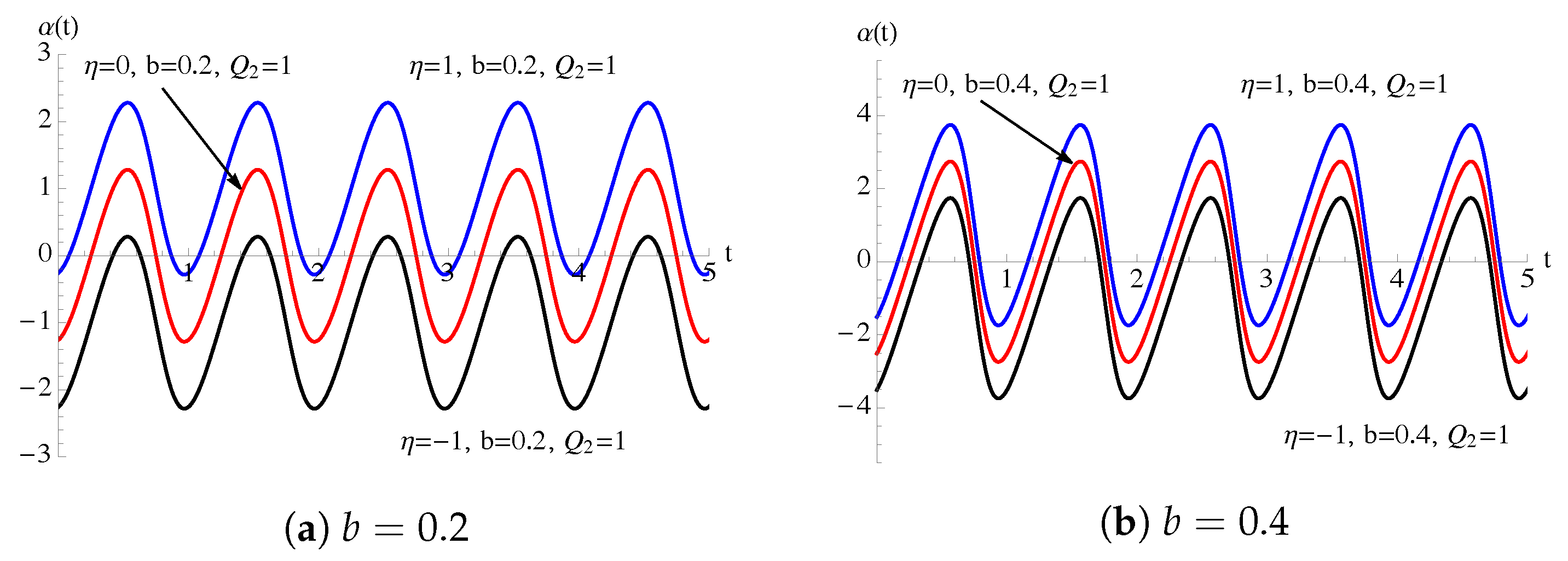
5.1. Periodic Immigration Intensity Function

We consider the time-inhomogeneous Feller process $X\left(t\right)$ such that

$$A_1(x,t)=\alpha x+\xi r\left(t\right),A_2(x,t)=2r\left(t\right)x,$$

(44)

with $\alpha \in \mathbb{R}$, $\xi >0$ and a zero-flux condition in the zero-state. We assume that $r\left(t\right)$ is a periodic function of period $Q_1$. From (15) for $n=0,1,\dots$ one has $A(t+n{Q}_1|t_0)=\alpha (t+n{Q}_1-t_0)$ and

$$\begin{array}{ccc}& & R(t+n{Q}_1|t_0)={\int }_{t_0}^{t+n{Q}_1}r\left(\tau \right)e^{-A\left(\tau \right|t_0)}d\tau \hfill \\ & & =e^{\alpha t_0}\left\{\frac{1-e^{-n\alpha Q_1}}{1-e^{-\alpha Q_1}}{\int }_{t_0}^{t_0+Q_1}r\left(\tau \right)e^{-\alpha \tau }d\tau +e^{-n\alpha Q_1}{\int }_{t_0}^{t}r\left(\tau \right)e^{-\alpha \tau }d\tau \right\}.\hfill \end{array}$$

If $\alpha <0$, the process $X\left(t\right)$ admits an asymptotic behavior. In this case, from (23), one has:

$$W(x,t)=\underset{n\to +\infty }{lim}f(x,t+n{Q}_1|x_0,t_0)=\frac{1}{x\Gamma \left(\xi \right)}{\left[{\psi }_1\left(t\right)x\right]}^{\xi }{e}^{-{\psi }_1\left(t\right)x},x\ge 0,$$

(45)

where

$${\psi }_1\left(t\right)=\underset{n\to +\infty }{lim}\frac{e^{-A(t+n{Q}_1|t_0)}}{R(t+n{Q}_1|t_0)}=\frac{e^{\left|\alpha \right|Q_1}-1}{R(t+Q_1|t)},\alpha <0.$$

(46)

We note that (45) is a gamma density of parameters $\xi$ and ${\left[{\psi }_1\left(t\right)\right]}^{-1}$ for all $t\ge 0$, so that for $\alpha <0$ it follows:

$$M_k\left(t\right)=\underset{n\to +\infty }{lim}\mathrm{E}\left\{{\left[X(t+n{Q}_1)\right]}^k\right|X\left(t_0\right)=x_0\}={\left[{\psi }_1\left(t\right)\right]}^{-k}{\left(\xi \right)}_k,k=1,2,\dots ,$$

(47)

with ${\psi }_1\left(t\right)$ given in (46).

Example 1.

The dynamic of a population influenced by seasonal immigration and regular environmental cycles, can be described by the time-inhomogeneous Feller process (44), with

$$r\left(t\right)=\nu \left[1+csin\left(\frac{2\pi t}{Q_1}\right)\right],t\ge 0,$$

(48)

where $\nu >0$ is the average of the periodic function $r\left(t\right)$ of period $Q_1$, c is the amplitude of the oscillations, with $0\le c<1$. These choices of parameters ensure that the both the immigration intensity function and the environment noise are positive functions. From (15), for $t\ge t_0$ one has $A\left(t\right|t_0)=\alpha (t-t_0)$ and

$$R\left(t\right|t_0)=\left\{\begin{array}{cc}\nu (t-t_0)+\frac{c\nu Q_1}{2\pi }\left[cos\left(\frac{2\pi t_0}{Q_1}\right)-cos\left(\frac{2\pi t}{Q_1}\right)\right],\hfill & \alpha =0,\hfill \\ \\ \frac{\nu }{\alpha }\left(1-e^{-\alpha (t-t_0)}\right)+\frac{c\nu Q_1}{4{\pi }^2+Q_1^2{\alpha }^2}\{2\pi cos\left(\frac{2\pi t_0}{Q_1}\right)\hfill \\ +\alpha Q_{1}sin\left(\frac{2\pi t_0}{Q_1}\right)-e^{-\alpha (t-t_0)}\left[2\pi cos\left(\frac{2\pi t}{Q_1}\right)+\alpha Q_{1}sin\left(\frac{2\pi t}{Q_1}\right)\right]\},\hfill & \alpha \ne 0.\hfill \end{array}\right.$$

For $\alpha <0$, the asymptotic density and the asymptotic moments are given in (45) and (47), respectively, with

$${\psi }_1\left(t\right)=\frac{1}{\nu }{\left\{\frac{1}{\left|\alpha \right|}-\frac{c{Q}_1}{4{\pi }^2+Q_1^2{\alpha }^2}\left[2\pi cos\left(\frac{2\pi t}{Q_1}\right)+\alpha Q_{1}sin\left(\frac{2\pi t}{Q_1}\right)\right]\right\}}^{-1}.$$

In Figure 1, Figure 2, Figure 3, Figure 4 and Figure 5, we consider the process (44); we assume that $r\left(t\right)=0.5\left[1+0.9sin\left(\pi t\right)\right]$ and that at the initial time $t_0=0$ the size of population is $X\left(t_0\right)=x_0=5$. We recall that $\alpha <0$ ($\alpha >0$) means that the birth intensity of the population is less (greater) than the death intensity. In Figure 1 and Figure 2 we assume that $\alpha =-0.05$, so that the process admits an asymptotic behavior. Specifically, in Figure 1, for $\xi =1.5$ the transition pdf of $X\left(t\right)$ is plotted as function of x on the left and as function of t on the right; the dotted functions indicate the corresponding asymptotic densities given in (45). Furthermore, in Figure 2, the conditional mean and variance of the population size and the related asymptotic behaviors are shown as function of t for various choices of ξ. In Figure 3, Figure 4 and Figure 5 we assume that $\alpha =0.05$ (on the left) and $\alpha =0$ (on the right), so that $X\left(t\right)$ does not admit an asymptotic behavior being $\alpha \ge 0$. In particular, in Figure 3, for $\xi =0.6$ the transition densities of the process (44) are plotted as function of x. Finally, in Figure 4 and Figure 5, the conditional mean and variance are plotted as function of t for various choices of ξ; we note that the mean and the variance of the population size don’t have an upper bound as t increases.

5.2. Periodic Growth Intensity Function

We consider the time-inhomogeneous Feller process $X\left(t\right)$ such that

$$A_1(x,t)=\alpha \left(t\right)x+\xi r,A_2\left(x\right)=2rx,$$

(49)

with $r>0$, $\xi >0$ and a zero-flux condition in the zero-state. We assume that $\alpha \left(t\right)$ is a periodic function of period $Q_2$ and let

$$\overline{\alpha }=\frac{A(t+Q_2|t)}{Q_2}=\frac{1}{Q_2}{\int }_t^{t+Q_2}\alpha \left(\tau \right)d\tau$$

(50)

be the mean of $\alpha \left(t\right)$ in the period $Q_2$. From (15), for $n=0,1,\dots$ one has:

$$\begin{array}{ccc}& & A(t+n{Q}_2|t_0)={\int }_{t_0}^{t+n{Q}_2}\alpha \left(\tau \right)d\tau =nA(t_0+Q_2|t_0)+A\left(t\right|t_0)=n\overline{\alpha }{Q}_2+A\left(t\right|t_0),\hfill \\ & & R(t+n{Q}_2|t_0)=r{\int }_{t_0}^{t+n{Q}_2}{e}^{-A\left(\tau \right|t_0)}d\tau \hfill \\ & & =r\left\{\frac{1-e^{-n\overline{\alpha }{Q}_2}}{1-e^{\overline{\alpha }{Q}_2}}{\int }_{t_0}^{t_0+Q_2}{e}^{-A\left(\tau \right|t_0)}d\tau +e^{-n\overline{\alpha }{Q}_2}{\int }_{t_0}^t{e}^{-A\left(\tau \right|t_0)}d\tau \right\}.\hfill \end{array}$$

If $\overline{\alpha }<0$, the process $X\left(t\right)$ admits an asymptotic behavior and, from (23), one has:

$$W(x,t)=\underset{n\to +\infty }{lim}f(x,t+n{Q}_2|x_0,t_0)=\frac{1}{x\Gamma \left(\xi \right)}{\left[{\psi }_2\left(t\right)x\right]}^{\xi }{e}^{-{\psi }_2\left(t\right)x},x\ge 0,$$

(51)

where

$${\psi }_2\left(t\right)=\underset{n\to +\infty }{lim}\frac{e^{-A(t+n{Q}_2|t_0)}}{R(t+n{Q}_2|t_0)}=\frac{e^{|\overline{\alpha }|Q_2}-1}{R(t+Q_2|t)},\overline{\alpha }<0.$$

(52)

We note again that (51) is a gamma density of parameters $\xi$ and ${\left[{\psi }_2\left(t\right)\right]}^{-1}$ for all $t\ge 0$; hence, for $\overline{\alpha }<0$ we have:

$$M_k\left(t\right)=\underset{n\to +\infty }{lim}\mathrm{E}\left\{{\left[X(t+n{Q}_2)\right]}^k\right|X\left(t_0\right)=x_0\}={\left[{\psi }_2\left(t\right)\right]}^{-k}{\left(\xi \right)}_k,k=1,2,\dots ,$$

(53)

with ${\psi }_2\left(t\right)$ given in (52).

Example 2.

For the time-inhomogeneous Feller process (49), we consider the flexible growth intensity function

$$\alpha \left(t\right)=\eta -\frac{2\pi b}{Q_2}\frac{cos\left(\frac{2\pi t}{Q_2}\right)}{1+bsin\left(\frac{2\pi t}{Q_2}\right)},t\ge 0,$$

(54)

where $\eta \in \mathbb{R}$, $Q_2$ is the period of $\alpha \left(t\right)$ and b determines the amplitude of the oscillations, with $0\le b<1$. As shown in Figure 6, the growth intensity function (54) can be positive, negative or zero at different time instants; furthermore, different choices of the parameter b make the function (54) less or more asymmetric in a period. Hence, the variety of shapes exhibits by $\alpha \left(t\right)$ allows to model several population growth trends.

From (15), making use of (54), for $t\ge t_0$ one obtains the following cumulative growth intensity function

$$A\left(t\right|t_0)=\eta (t-t_0)-ln\left[1+bsin\left(\frac{2\pi t}{Q_2}\right)\right]+ln\left[1+bsin\left(\frac{2\pi t_0}{Q_2}\right)\right]$$

(55)

and hence

$$R\left(t\right|t_0)=\left\{\begin{array}{cc}\frac{r}{1+bsin\left(\frac{2\pi t_0}{Q_2}\right)}\left\{t-t_0-\frac{b{Q}_2}{2\pi }\left[cos\left(\frac{2\pi t}{Q_2}\right)-cos\left(\frac{2\pi t_0}{Q_2}\right)\right]\right\},\hfill & \eta =0,\hfill \\ \\ \frac{r}{1+bsin\left(\frac{2\pi t_0}{Q_2}\right)}\{\frac{1-e^{-\eta (t-t_0)}}{\eta }-\frac{2\pi b{Q}_2}{4{\pi }^2+Q_2^2{\eta }^2}[e^{-\eta (t-t_0)}cos\left(\frac{2\pi t}{Q_2}\right)\hfill \\ +\frac{Q_2\eta }{2\pi }{e}^{-\eta (t-t_0)}sin\left(\frac{2\pi t}{Q_2}\right)-cos\left(\frac{2\pi t_0}{Q_2}\right)-\frac{Q_2\eta }{2\pi }sin\left(\frac{2\pi t_0}{Q_2}\right)\},\hfill & \eta \ne 0.\hfill \end{array}\right.$$

(56)

From (50) and (54) we have $\overline{\alpha }=\eta$, so that $X\left(t\right)$ admits an asymptotic behavior for $\eta <0$; the asymptotic density and the asymptotic moments are given in (51) and (53), respectively, with

$${\psi }_2\left(t\right)=\frac{1}{r}\left[1+bsin\left(\frac{2\pi t}{Q_2}\right)\right]{\left\{\frac{1}{\left|\eta \right|}-\frac{2\pi b{Q}_2}{4{\pi }^2+Q_2^2{\eta }^2}\left[cos\left(\frac{2\pi t}{Q_2}\right)+\frac{Q_2\eta }{2\pi }sin\left(\frac{2\pi t}{Q_2}\right)\right]\right\}}^{-1}.$$

In Figure 7, Figure 8, Figure 9, Figure 10 and Figure 11, we consider the process (49) with $r=1$ and $\alpha \left(t\right)=\eta -0.4\pi cos\left(2\pi t\right){\left[1+0.2sin\left(2\pi t\right)\right]}^{-1}$; furthermore, we assume that at the initial time $t_0=0$ the size of population is $X\left(t_0\right)=x_0=5$. We note that $\eta <0$ ($\eta >0$) indicates that the average of birth intensity of the population is less (greater) than the average of the death intensity. In Figure 7 and Figure 8 we assume that $\eta =-1$, so that the process admits an asymptotic behavior. In particular, in Figure 7, for $\xi =1.5$ the transition pdf of $X\left(t\right)$ is plotted as function of x on the left and as function of t on the right; the dotted functions indicate the corresponding asymptotic densities, given in (51). Furthermore, in Figure 8 the conditional mean and variance and the related asymptotic behaviors are plotted as function of t for various choices of ξ. Instead, in Figure 9, Figure 10 and Figure 11 we assume that $\eta =1$ on the left and $\eta =0$ on the right. Specifically, in Figure 9, the transition densities of the process (49), for $\xi =1.5$ are shown as function of x. Finally, in Figure 10 and Figure 11 the conditional mean and variance of the population size are plotted as function of t for various choices of ξ.

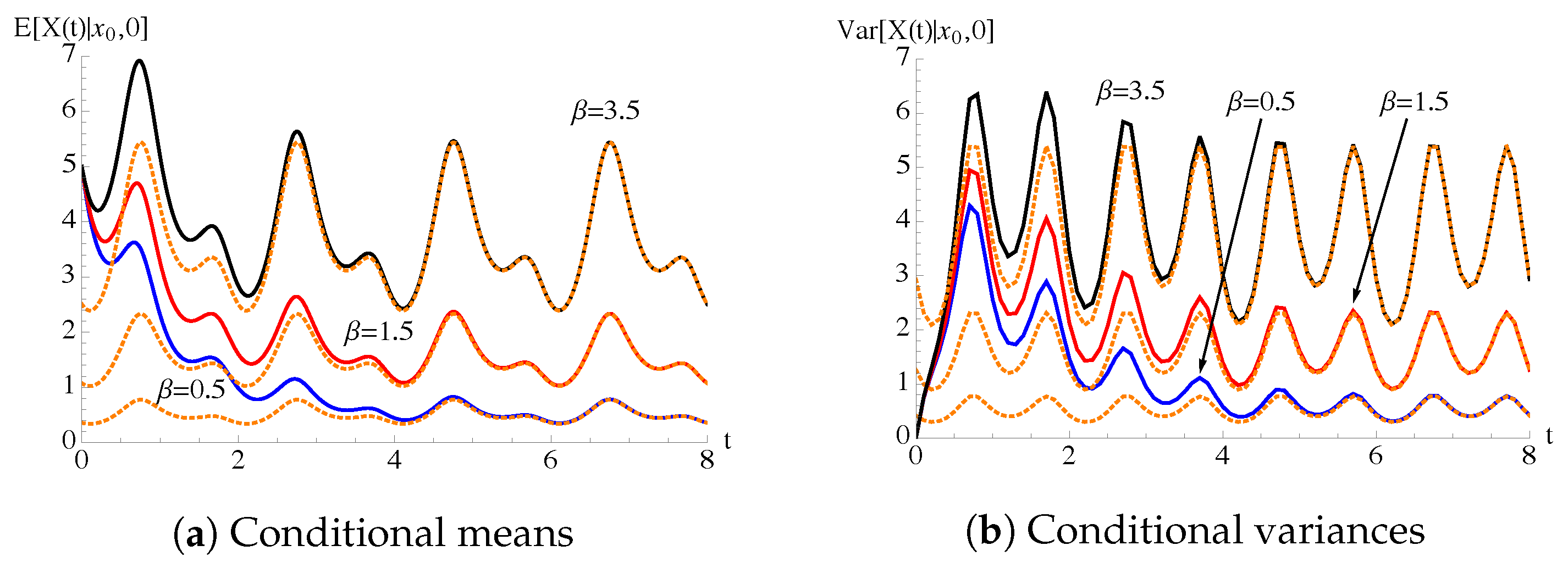
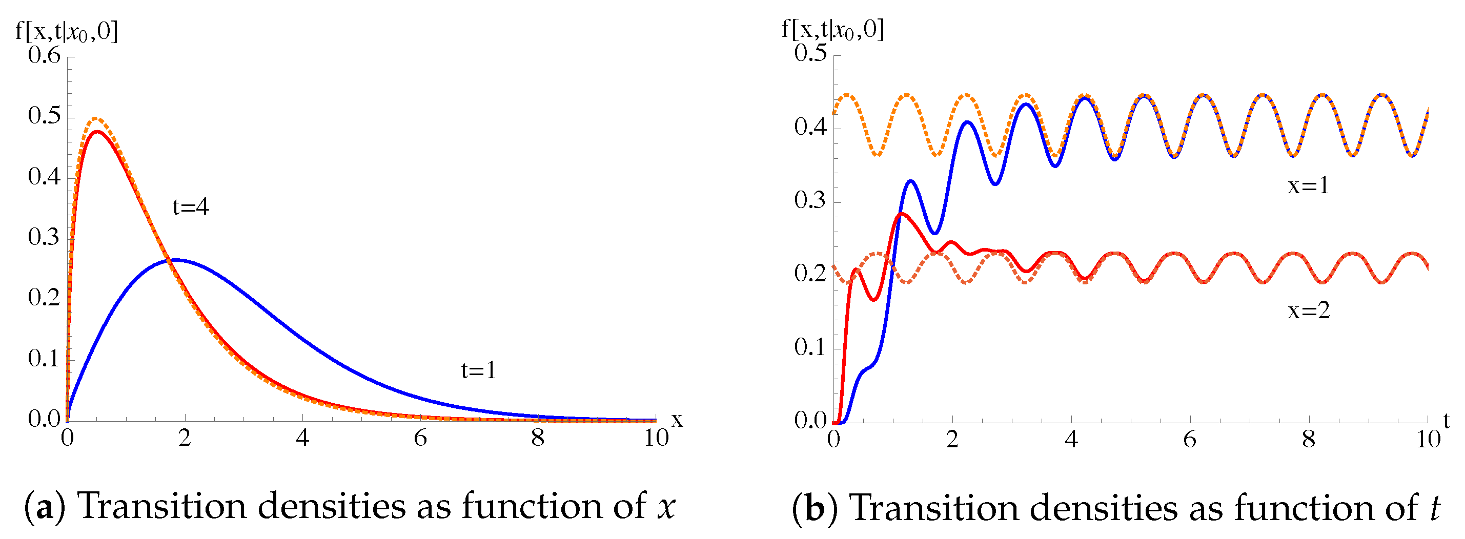
5.3. Periodic Immigration and Growth Intensity Functions

We consider the process $X\left(t\right)$ such that

$$A_1(x,t)=\alpha \left(t\right)x+\xi r\left(t\right),A_2(x,t)=2r\left(t\right)x,$$

(57)

with $\xi >0$ and a zero-flux condition in the zero-state. We assume that $r\left(t\right)$ and $\alpha \left(t\right)$ are periodic functions of periods $Q_1$ and $Q_2$, respectively. We denote by $Q=LCM(Q_1,Q_2)$ the least common multiple between $Q_1$ and $Q_2$ and let

$$\widehat{\alpha }=\frac{A(t+Q|t)}{Q}=\frac{1}{Q}{\int }_t^{t+Q}\alpha \left(\tau \right)d\tau =\frac{1}{Q_2}{\int }_t^{t+Q_2}\alpha \left(\tau \right)d\tau =\overline{\alpha }$$

be the mean of $\alpha \left(t\right)$ in Q. From (15) for $n=0,1,\dots$ one has:

$$\begin{array}{ccc}& & A(t+nQ|t_0)={\int }_{t_0}^{t+nQ}\alpha \left(\tau \right)d\tau =nA(t_0+Q|t_0)+A\left(t\right|t_0)=n\widehat{\alpha }Q+A\left(t\right|t_0),\hfill \\ & & R(t+nQ|t_0)={\int }_{t_0}^{t+nQ}r\left(\tau \right)e^{-A\left(\tau \right|t_0)}d\tau \hfill \\ & & =\frac{1-e^{-n\widehat{\alpha }Q}}{1-e^{-\widehat{\alpha }Q}}{\int }_{t_0}^{t_0+Q}r\left(\tau \right)e^{-A\left(\tau \right|t_0)}d\tau +e^{-n\widehat{\alpha }Q}{\int }_{t_0}^{t}r\left(\tau \right)e^{-A\left(\tau \right|t_0)}d\tau .\hfill \end{array}$$

If $\widehat{\alpha }<0$, the process $X\left(t\right)$ admits an asymptotic behavior and, from (23), one obtains the gamma density:

$$W(x,t)=\underset{n\to +\infty }{lim}f(x,t+nQ|x_0,t_0)=\frac{1}{x\Gamma \left(\xi \right)}{\left[{\psi }_3\left(t\right)x\right]}^{\xi }{e}^{-{\psi }_3\left(t\right)x},x\ge 0,$$

(58)

where

$${\psi }_3\left(t\right)=\underset{n\to +\infty }{lim}\frac{e^{-A(t+nQ|t_0)}}{R(t+nQ|t_0)}=\frac{e^{|\widehat{\alpha }|Q}-1}{R(t+Q|t)},\widehat{\alpha }<0.$$

(59)

Hence, for $\widehat{\alpha }<0$ we have:

$$M_k\left(t\right)=\underset{n\to +\infty }{lim}\mathrm{E}\left\{{\left[X(t+nQ)\right]}^k\right|X\left(t_0\right)=x_0\}={\left[{\psi }_3\left(t\right)\right]}^{-k}{\left(\xi \right)}_k,k=1,2,\dots ,$$

(60)

with ${\psi }_3\left(t\right)$ given in (59).

Example 3.

We consider a population described by the time-inhomogeneous Feller process (57) and we assume that the noise intensity $r\left(t\right)$ is defined in (48) and the growth intensity function $\alpha \left(t\right)$ is chosen as in (54). In this case, the cumulative growth intensity function $A\left(t\right|t_0)$ is given in (55) and

$$R\left(t\right|t_0)=\frac{\nu }{1+bsin\left(\frac{2\pi t_0}{Q_2}\right)}{\int }_{t_0}^t{e}^{-\eta (\tau -t_0)}\left[1+csin\left(\frac{2\pi \tau }{Q_1}\right)\right]\left[1+bsin\left(\frac{2\pi \tau }{Q_2}\right)\right]d\tau .$$

(61)

From (50) and (54) we have $\widehat{\alpha }=\eta$. For $\eta <0$, the asymptotic density and the asymptotic moments are given in (58) and (60), respectively, with

$${\psi }_3\left(t\right)=\frac{1}{\nu }\left[1+bsin\left(\frac{2\pi t}{Q_2}\right)\right]{\left\{\frac{1}{\left|\eta \right|}-c{Q}_1{B}_1\left(t\right)-b{Q}_2{B}_2\left(t\right)-\frac{bc{Q}_1{Q}_2}{2}[C\left(t\right)-D\left(t\right)]\right\}}^{-1},$$

where

$$\begin{array}{ccc}& & B_i\left(t\right)=\frac{2\pi cos\left(\frac{2\pi t}{Q_i}\right)+Q_i\eta sin\left(\frac{2\pi t}{Q_i}\right)}{4{\pi }^2+Q_i^2{\eta }^2},i=1,2,\hfill \\ & & C\left(t\right)=\frac{Q_1{Q}_2\eta cos\left(2\pi \frac{Q_1-Q_2}{Q_1{Q}_2}t\right)-2\pi (Q_1-Q_2)sin\left(2\pi \frac{Q_1-Q_2}{Q_1{Q}_2}t\right)}{4{\pi }^2{(Q_1-Q_2)}^2+Q_1^2{Q}_2^2{\eta }^2},\hfill \\ & & D\left(t\right)=\frac{Q_1{Q}_2\eta cos\left(2\pi \frac{Q_1+Q_2}{Q_1{Q}_2}t\right)-2\pi (Q_1+Q_2)sin\left(2\pi \frac{Q_1+Q_2}{Q_1{Q}_2}t\right)}{4{\pi }^2{(Q_1+Q_2)}^2+Q_1^2{Q}_2^2{\eta }^2}.\hfill \end{array}$$

In Figure 12, Figure 13, Figure 14, Figure 15 and Figure 16, we assume that the noise intensity function is $r\left(t\right)=0.5\left[1+0.9sin\left(\pi t\right)\right]$ and the growth intensity function is $\alpha \left(t\right)=\eta -0.4\pi cos\left(2\pi t\right){\left[1+0.2sin\left(2\pi t\right)\right]}^{-1}$; since $r\left(t\right)$ has period $Q_1=2$ and $\alpha \left(t\right)$ has period $Q_2=1$, one has $Q=LCM(Q_1,Q_2)=2$. Furthermore, the size of population at time $t_0=0$ is $X\left(0\right)=5$. In Figure 12 and Figure 13 we assume that $\eta =-1$, so that the process admits an asymptotic behavior. Specifically, in Figure 12, for $\xi =1.5$ the transition pdf of the process (57) is plotted as function of x on the left and as function of t on the right; the dotted functions indicate the corresponding asymptotic densities, given in (51). Furthermore, in Figure 13 the conditional mean and variance and the related asymptotic behaviors are plotted as function of t for various choices of ξ. Comparing Figure 8 and Figure 13 we can highlight the effect of the periodic noise intensity on the conditional mean and variance of the population size for a fixed periodic growth intensity function. In Figure 14, Figure 15 and Figure 16, we consider $\eta =1$ on the left and $\eta =0$ on the right; in these cases the process does not exhibit an asymptotic behavior, being $\eta \ge 0$. In Figure 14, for $\xi =1.5$ the transition densities of the process are plotted as function of x. Finally, in Figure 15 and Figure 16 the conditional mean and variance of the population size are shown as function of t for various choices of ξ.

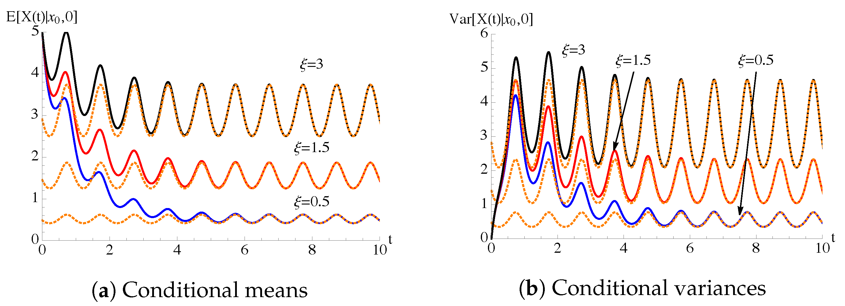
5.4. Periodic Immigration, Growth and Noise Intensity Functions

We consider the time-inhomogeneous Feller process $X\left(t\right)$ having infinitesimal moments (1), with a zero-flux condition in the zero-state. We assume that $r\left(t\right)$, $\alpha \left(t\right)$ and $\beta \left(t\right)$ are periodic functions of periods $Q_1$, $Q_2$ and $Q_3$, respectively. Some, but not all, of these functions can be constant. We denote by Q the least common multiple of the periods related to the periodic functions and by $\widehat{\alpha }$ the mean of $\alpha \left(t\right)$ in Q, so that relations in (58) hold.

If $\widehat{\alpha }<0$, the process $X\left(t\right)$ admits an asymptotic behavior. In this case, from (16) one obtains the asymptotic mean and variance:

$$\begin{array}{ccc}& & M_1\left(t\right)=\underset{n\to +\infty }{lim}\mathrm{E}\left\{X(t+nQ)\right|X\left(t_0\right)=x_0\}=\frac{1}{e^{|\widehat{\alpha }|Q}-1}{\int }_t^{t+Q}\beta \left(u\right)e^{-A\left(u\right|t)}du,\hfill \end{array}$$

$$\begin{array}{ccc}& & \hfill \\ & & V\left(t\right)=\underset{n\to +\infty }{lim}\mathrm{Var}\left\{X(t+nQ)\right|X\left(t_0\right)=x_0\}=\frac{2}{{(e^{|\widehat{\alpha }|Q}-1)}^2(1+e^{|\widehat{\alpha }|Q})}\hfill \end{array}$$

(62)

$$\begin{array}{ccc}& & \times {\int }_t^{t+Q}\beta \left(u\right)e^{-A\left(u\right|t)}\left[R\left(u\right|t)+e^{|\widehat{\alpha }|Q}{\int }_u^{t+Q}r\left(\tau \right)e^{-A\left(\tau \right|t)}d\tau \right]du.\hfill \end{array}$$

(63)

Note that if $\beta \left(t\right)=\xi r\left(t\right)$, from (62) and (63) one has $M_1\left(t\right)=\xi {\left[{\psi }_3\left(t\right)\right]}^{-1}$ and $V\left(t\right)=\xi {\left[{\psi }_3\left(t\right)\right]}^{-2}$, with ${\psi }_3\left(t\right)$ defined in (59).

Example 4.

We consider the process (1) and we assume that $\beta \left(t\right)=\beta >0$, $r\left(t\right)$ is given in (48) and $\alpha \left(t\right)$ is defined in (54). In this case, the immigration rate is constant, whereas the growth and the noise intensity functions are periodic functions with different periods. Expressions (55) and (61) for $A\left(t\right|t_0)$ and $R\left(t\right|t_0)$ hold. Furthermore, from (50) and (54) we have $\widehat{\alpha }=\eta$, so that for $\eta <0$ the process admits an asymptotic behavior.

We assume that the noise intensity function $r\left(t\right)$ has period $Q_1=2$ and the growth intensity function $\alpha \left(t\right)$ has period $Q_2=1$, so that $Q=LCM(Q_1,Q_2)=2$. In Figure 17, the conditional mean and variance and the related asymptotic behaviors are plotted as function of t for various choices of β. We note that the conditional mean is not affect to the periodicity of $r\left(t\right)$, whereas the conditional variance depends on the different periodicities of the growth intensity function $\alpha \left(t\right)$ and of the noise intensity function $r\left(t\right)$.

Example 5.

We consider the process (1) and we assume that $r\left(t\right)=r>0$, $\alpha \left(t\right)$ is defined in (54) and

$$\beta \left(t\right)=\beta \left[1+csin\left(\frac{2\pi t}{Q_1}\right)\right],t\ge 0,$$

(64)

where $\beta >0$ is the average of the periodic function $\beta \left(t\right)$ of period $Q_1$, c is the amplitude of the oscillations, with $0\le c<1$. Differently from Example 4, the noise intensity is constant, whereas the growth and the immigration intensity functions are periodic functions with different periods. Expressions (55) and (56) for $A\left(t\right|t_0)$ and $R\left(t\right|t_0)$ hold. Furthermore, from (50) and (54) we have $\widehat{\alpha }=\eta$, so that for $\eta <0$ the process admits an asymptotic behavior.

We assume that the immigration intensity function $\beta \left(t\right)$, given in (64), has period $Q_1=2$ and the growth intensity function $\alpha \left(t\right)$ has period $Q_2=1$, so that $Q=LCM(Q_1,Q_2)=2$. In Figure 18, the conditional mean and variance and the related asymptotic behaviors are plotted as function of t for various choices of β. We note that both the mean and the variance depend on the periodicities of the intensity functions $\alpha \left(t\right)$ and $\beta \left(t\right)$.

6. Concluding Remarks

In this paper, we considered a time-inhomogeneous Feller-type diffusion process $\{X\left(t\right),t\ge t_0\}$, $t_0\ge 0$, with infinitesimal drift $A_1(x,t)=\alpha \left(t\right)x+\beta \left(t\right)$ and infinitesimal variance $A_2(x,t)=2r\left(t\right)x$, defined in the state-space $[0,+\infty )$, with a zero-flux condition in the zero-state. We have assumed that $\alpha \left(t\right)\in \mathbb{R}$, $\beta \left(t\right)\ge 0$, $r\left(t\right)>0$ for all $t\ge t_0$. This diffusion process plays a relevant role in several biological applications and can be derived as the continuous approximation of the time-inhomogeneous birth-death process with immigration. In the general case, the transition density and the conditional moments are explicitly obtained. Some special situations are analyzed: (i) the absence of immigration with $\beta \left(t\right)=0$, (ii) the proportional case in which $\beta \left(t\right)=\xi r\left(t\right)$, with $\xi >0$, and (iii) the time-homogeneous case. Sometimes in the dynamics of populations it is necessary to consider periodic intensity functions. Indeed, periodic immigration and periodic growth intensity functions play an important role in the description of the evolution of dynamic systems influenced by seasonal immigration or other regular environmental cycles. Furthermore, the population dynamics can be affected by noise of periodic intensity. Therefore, we have assumed that the growth intensity function $\alpha \left(t\right)$, or the immigration intensity function $\beta \left(t\right)$ or the noise intensity $r\left(t\right)$ have some kind of periodicity. In these cases, the asymptotic behaviors of the transition pdf and of the moments are discussed. Various numerical computations are performed to analyze how the population dynamics is affected by the periodic intensity functions.

References

1. Bharucha-Reid, A.T. Elements of the Theory of Markov Processes and Their Applications; McGraw-Hill: New York, NY, USA, 1960. [Google Scholar]
2. Cox, D.R.; Miller, H.D. The Theory of Stochastic Processes; Chapman & Hall/CRC: Boca Raton, FL, USA, 1996. [Google Scholar]
3. Ricciardi, L.M. Diffusion Processes and Related Topics in Biology; Springer: Berlin, Germany, 1977. [Google Scholar]
4. Ricciardi, L.M. Stochastic Population Theory: Diffusion Processes. In Mathematical Ecology; Hallam, T.G., Levin, S.A., Eds.; Springer: Berlin, Germany, 1986; Volume 17, pp. 191–238. [Google Scholar]
5. Tuckwell, H.C. Introduction to Theoretical Neurobiology: Volume 2, Nonlinear and Stochastic Theories; Cambridge University Press: Cambridge, MA, USA, 1988. [Google Scholar]
6. Gardiner, C.W. Handbook of Stochastic Methods: For Physics, Chemistry and the Natural Sciences; Springer: Berlin, Germany, 1985. [Google Scholar]
7. Feller, W. Diffusion processes in genetics. In Proceedings of the Second Berkeley Symposium on Mathematical Statistics and Probability; Statistical Laboratory of the University of California: Berkeley, CA, USA, 1951; pp. 227–246. [Google Scholar]
8. Ricciardi, L.M.; Di Crescenzo, A.; Giorno, V.; Nobile, A.G. An outline of theoretical and algorithmic approaches to first passage time problems with applications to biological modeling. Math. Jpn. 1999, 50, 247–322. [Google Scholar]
9. Pugliese, A.; Milner, F. A structured population model with diffusion in structure space. J. Math. Biol. 2018, 77, 2079–2102. [Google Scholar] [CrossRef] [Green Version]
10. Masoliver, J.; Perelló, J. First-passage and escape problems in the Feller process. Phys. Rev. E 2012, 86, 041116. [Google Scholar] [CrossRef] [Green Version]
11. Masoliver, J. Nonstationary Feller process with time-varying coefficients. Phys. Rev. E 2016, 93, 012122. [Google Scholar] [CrossRef] [PubMed] [Green Version]
12. Di Crescenzo, A.; Nobile, A.G. Diffusion approximation to a queueing system with time-dependent arrival and service rates. Queueing Syst. 1995, 19, 41–62. [Google Scholar] [CrossRef]
13. Sacerdote, L. On the solution of the Fokker-Planck equation for a Feller process. Adv. Appl. Prob. 1990, 22, 101–110. [Google Scholar] [CrossRef]
14. Ditlevsen, S.; Lánský, P. Estimation of the input parameters in the Feller neuronal model. Phys. Rev. E 2006, 73, 061910. [Google Scholar] [CrossRef] [PubMed]
15. Buonocore, A.; Giorno, V.; Nobile, A.G.; Ricciardi, L.M. A neuronal modeling paradigm in the presence of refractoriness. BioSystems 2002, 67, 35–43. [Google Scholar] [CrossRef]
16. Giorno, V.; Lánský, P.; Nobile, A.G.; Ricciardi, L.M. Diffusion approximation and first-passage-time problem for a model neuron. III. A birth-and-death process approach. Biol. Cyber. 1988, 58, 387–404. [Google Scholar] [CrossRef] [Green Version]
17. Nobile, A.G.; Pirozzi, E. On time non-homogeneous Feller-type diffusion process in neuronal modeling. In Computer Aided Systems Theory—Eurocast 2015; Moreno-Díaz, R., Pichler, F., Eds.; Lecture Notes in Computer Science; Springer International Publishing: Cham, Switzerland, 2015; Volume 9520, pp. 183–191. [Google Scholar]
18. D’Onofrio, G.; Lánský, P.; Pirozzi, E. On two diffusion neuronal models with multiplicative noise: The mean first-passage time properties. Chaos 2018, 28, 043103. [Google Scholar] [CrossRef]
19. Tian, Y.; Zhang, H. Skew CIR process, conditional characteristic function, moments and bond pricing. Appl. Math. Comput. 2018, 329, 230–238. [Google Scholar] [CrossRef]
20. Cox, J.C.; Ingersoll, J.E., Jr.; Ross, S.A. A theory of the term structure of interest rates. Econometrica 1985, 53, 385–407. [Google Scholar] [CrossRef]
21. Maghsoodi, Y. Solution of the extended CIR term structure and bond option valuation. Math. Financ. 1996, 6, 89–109. [Google Scholar] [CrossRef]
22. Peng, Q.; Schellhorn, H. On the distribution of extended CIR model. Stat. Probab. Lett. 2018, 142, 23–29. [Google Scholar] [CrossRef]
23. Linetsky, V. Computing hitting time densities for CIR and OU diffusions. Applications to mean-reverting models. J. Comput. Financ. 2004, 7, 1–22. [Google Scholar] [CrossRef] [Green Version]
24. Di Nardo, E.; D’Onofrio, G. A cumulant approach for the first-passage-time problem of the Feller square-root process. Appl. Math. Comput. 2021, 391, 125707. [Google Scholar]
25. Lavigne, F.; Roques, L. Extinction times of an inhomogeneous Feller diffusion process: A PDF approach. Expo. Math. 2021, 39, 137–142. [Google Scholar] [CrossRef]
26. Giorno, V.; Nobile, A.G. Time-inhomogeneous Feller-type diffusion process with absorbing boundary condition. J. Stat. Phys. 2021, 183, 1–27. [Google Scholar]
27. Bhattacharya, R.N.; Waymire, E.C. Stochastic Processes with Applications; Classics in Applied Mathematics; SIAM: Philadelphia, PA, USA, 2009. [Google Scholar]
28. Giorno, V.; Nobile, A.G. Bell polynomial approach for time-inhomogeneous linear birth-death process with immigration. Mathematics 2020, 8, 1123. [Google Scholar] [CrossRef]
29. Di Crescenzo, A.; Giorno, V.; Krishna Kumar, B.; Nobile, A.G. A double-ended queue with catastrophes and repairs, and a jump-diffusion approximation. Methodol. Comput. Appl. Probab. 2012, 14, 937–954. [Google Scholar] [CrossRef] [Green Version]
30. Di Crescenzo, A.; Giorno, V.; Krishna Kumar, B.; Nobile, A.G. A time-non-homogeneous double-ended queue with failures and repairs and its continuous approximation. Mathematics 2018, 6, 81. [Google Scholar] [CrossRef] [Green Version]
31. Dharmaraja, S.; Di Crescenzo, A.; Giorno, V.; Nobile, A.G. A continuous-time Ehrenfest model with catastrophes and its jump-diffusion approximation. J. Stat. Phys. 2015, 161, 326–345. [Google Scholar] [CrossRef]
32. Gan, X.; Waxman, D. Singular solution of the Feller diffusion equation via a spectral decomposition. Phys. Rev. E Stat. Nonlin. Soft. Matter Phys. 2015, 91, 012123. [Google Scholar] [CrossRef]
33. Abramowitz, I.A.; Stegun, M. Handbook of Mathematical Functions; Dover Publications, Inc.: New York, NY, USA, 1972. [Google Scholar]
34. Feller, W. Two singular diffusion problems. Ann. Math. 1951, 54, 173–182. [Google Scholar] [CrossRef]
35. Feller, W. The parabolic differen tial equations and the associated semi-groups of transformations. Ann. Math. 1952, 55, 468–518. [Google Scholar] [CrossRef]
36. Karlin, S.; Taylor, H.W. A Second Course in Stochastic Processes; Academic Press: New York, NY, USA, 1981. [Google Scholar]
37. Giorno, V.; Nobile, A.G.; Ricciardi, L.M.; Sacerdote, L. Some remarks on the Rayleigh process. J. Appl. Prob. 1986, 23, 398–408. [Google Scholar] [CrossRef]
38. Gradshteyn, I.S.; Ryzhik, I.M. Table of Integrals, Series and Products; Academic Press Inc.: Cambridge, MA, USA, 2014. [Google Scholar]
39. Erdèlyi, A.; Magnus, W.; Oberthettinger, F.; Tricomi, F.G. Higher Trascendental Functions; Mc Graw-Hill: New York, NY, USA, 1953; Volume II. [Google Scholar]
40. Coleman, B.D.; Hsieh, Y.-H.; Knowles, G.P. On the optimal choice of r for a population in a periodic environment. Math. Biosci. 1979, 46, 71–85. [Google Scholar] [CrossRef]
41. Keeling, M.J.; Rohani, P. Modeling Infectious Diseases in Humans and Animals; Princeton University Press: Princeton, NJ, USA, 2008. [Google Scholar]
42. Williams, W.E. Partial Differential Equations; Clarendon Press: Oxford, UK, 1980. [Google Scholar]
43. Erdèlyi, A.; Magnus, W.; Oberthettinger, F.; Tricomi, F.G. Tables of Integral Transforms; Mc Graw-Hill: New York, NY, USA, 1954; Volume 1. [Google Scholar]
44. Comtet, L. Advanced Combinatorics: The Art of Finite and Infinite Expansions; D. Reidel Publishing Company: Dordrecht, The Netherlands; Boston, MA, USA, 1974. [Google Scholar]
Figure 1. For the process (44), with x0 = 5, α = 0.05, ξ = 1.5 and r(t) = 0.51[1 + 0.9 sin(πt)], the transition densities are plotted. The dotted functions indicate the corresponding asymptotic densities.
Mathematics 09 01879 g001
Figure 2. For the process of Figure 1, the conditional means and variances are plotted as function of t for various choices of ξ. The dotted functions indicate the corresponding asymptotic means and variances.
Mathematics 09 01879 g002
Figure 3. For the process (44), with x0 = 5, ξ = 0.6 and r(t) = 0.51[1 + 0.9 sin(πt)], the transition densities are plotted as function of x.
Mathematics 09 01879 g003
Figure 4. For the process of Figure 3, the conditional means are plotted as function of t for various choices of ξ.
Mathematics 09 01879 g004
Figure 5. For the process of Figure 3, the conditional variances are plotted as function of t for various choices of ξ.
Mathematics 09 01879 g005
Figure 6. The growth intensity function α(t), given in (54), is plotted as function of t for some choices of the parameters.
Mathematics 09 01879 g006
Figure 7. For the process (49), with x0 = 5, r = 1, ξ = 1.5, η = −1 and α(t) = η − 0.4π cos(2πt) [1 + 0.2 sin(2πt)]−1, the transition densities are plotted. The dotted functions indicate the corresponding asymptotic densities.
Mathematics 09 01879 g007
Figure 8. For the process of Figure 7, the conditional means and variances are plotted as function of t for various choices of ξ. The dotted functions indicate the related asymptotic means and variances.
Mathematics 09 01879 g008
Figure 9. For the process of Figure 7, the transition densities are plotted as function of x.
Mathematics 09 01879 g009
Figure 10. For the process of Figure 7, the conditional means are plotted as function of t for various choices of ξ.
Mathematics 09 01879 g010
Figure 11. For the process of Figure 7, the conditional variances are plotted as function of t for various choices of ξ.
Mathematics 09 01879 g011
Figure 12. For the process (57), with x0 = 5, ξ = 1.5, η = −1, α(t) = η − 0.4π cos(2πt) [1 + 0.2 sin(2πt)]−1 and r(t) = 0.5[1 + 0.9 sin(πt)], the transition densities are plotted. The dotted functions indicate the related asymptotic densities.
Mathematics 09 01879 g012
Figure 13. For the process of Figure 12, the conditional means and the conditional variances are plotted as function of t for various choices of ξ. The dotted functions indicate the corresponding asymptotic means and variances.
Mathematics 09 01879 g013
Figure 14. For the process of Figure 12, the transition densities are plotted as function of x.
Mathematics 09 01879 g014
Figure 15. For the process of Figure 12, the conditional means are plotted as function of t for various choices of ξ.
Mathematics 09 01879 g015
Figure 16. For the process of Figure 12, the conditional variances are plotted as function of t for various choices of ξ.
Mathematics 09 01879 g016
Figure 17. For the process (1), with x0 = 5, η = −1, α(t) = η − 0.4π cos(2πt) [1 + 0.2 sin(2πt)]−1 and r(t) = 0.5[1 + 0.9 sin(πt)], the conditional means and variances are plotted as function of t for various choices of β. The dotted functions indicate the corresponding asymptotic means and variances.
Mathematics 09 01879 g017
Figure 18. For the process (1), with x0 = 5, η = −1, r = 1, α(t) = η − 0.4π cos(2πt) [1 + 0.2 sin(2πt)]−1 and β(t) = β[1 + 0.9 sin(πt)], the conditional means and variances are plotted as function of t for various choices of β. The dotted functions indicate the related asymptotic means and variances.
Mathematics 09 01879 g018
Publisher’s Note: MDPI stays neutral with regard to jurisdictional claims in published maps and institutional affiliations.