
Spectral Properties of Clipping Noise


Abstract
:1. Introduction
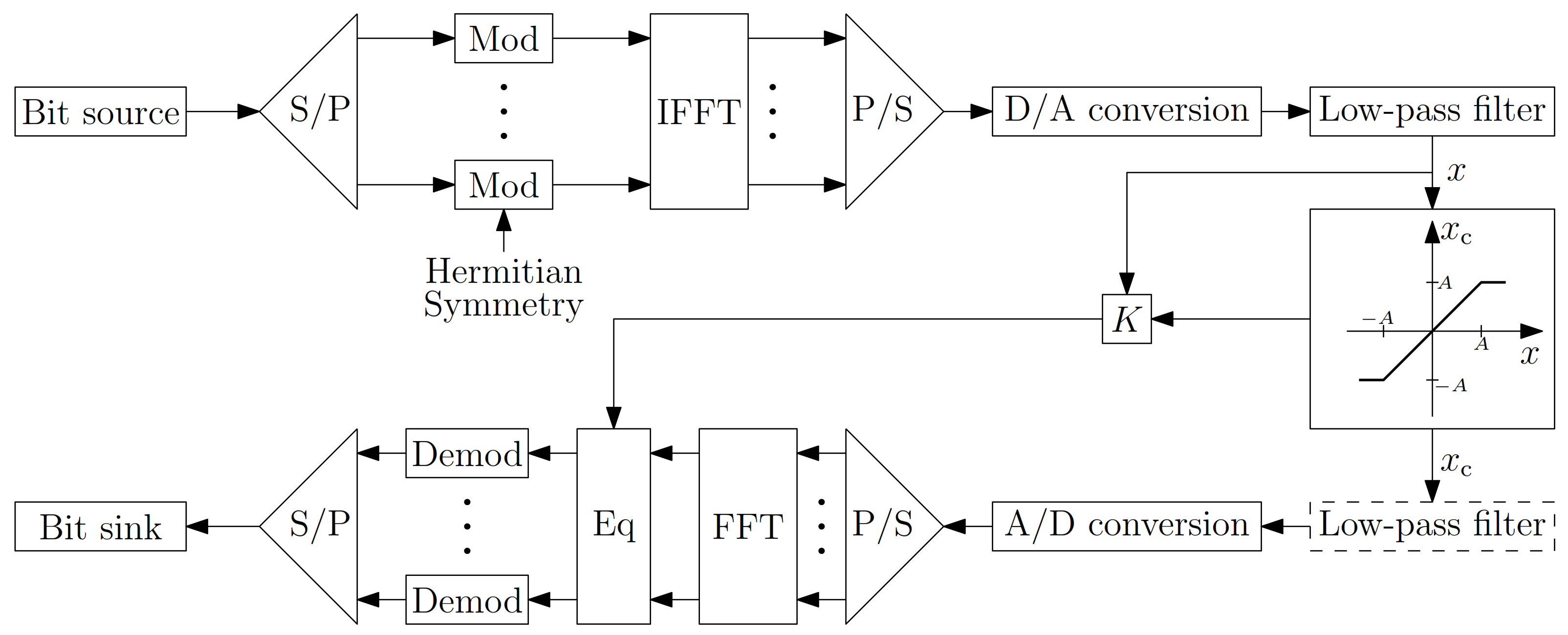
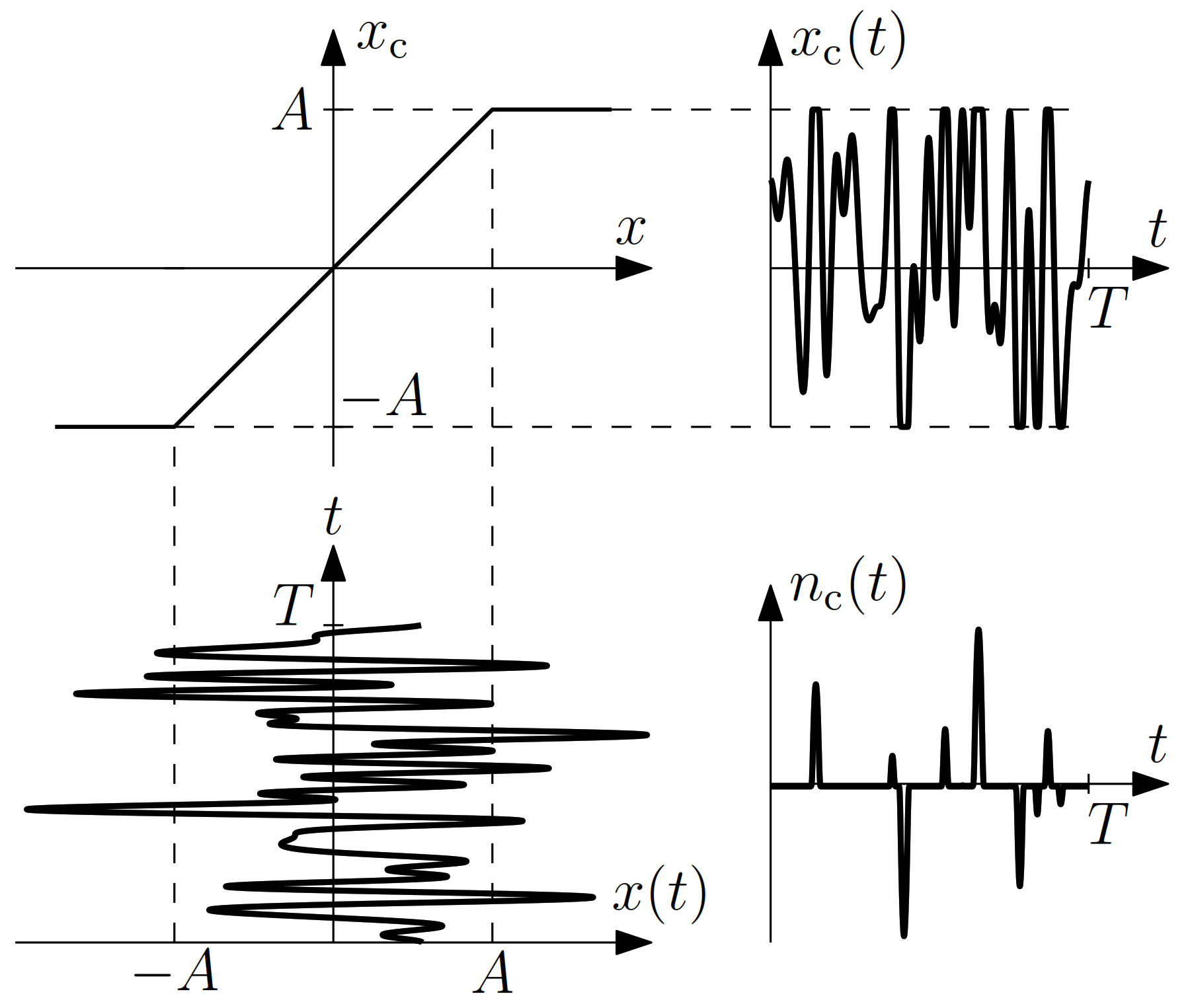
2. System Model
3. Review of the Bussgang Theorem
3.1. Mathematical Derivation of the Bussgang Theorem
3.1.1. Calculation of the Linear Damping Factor K
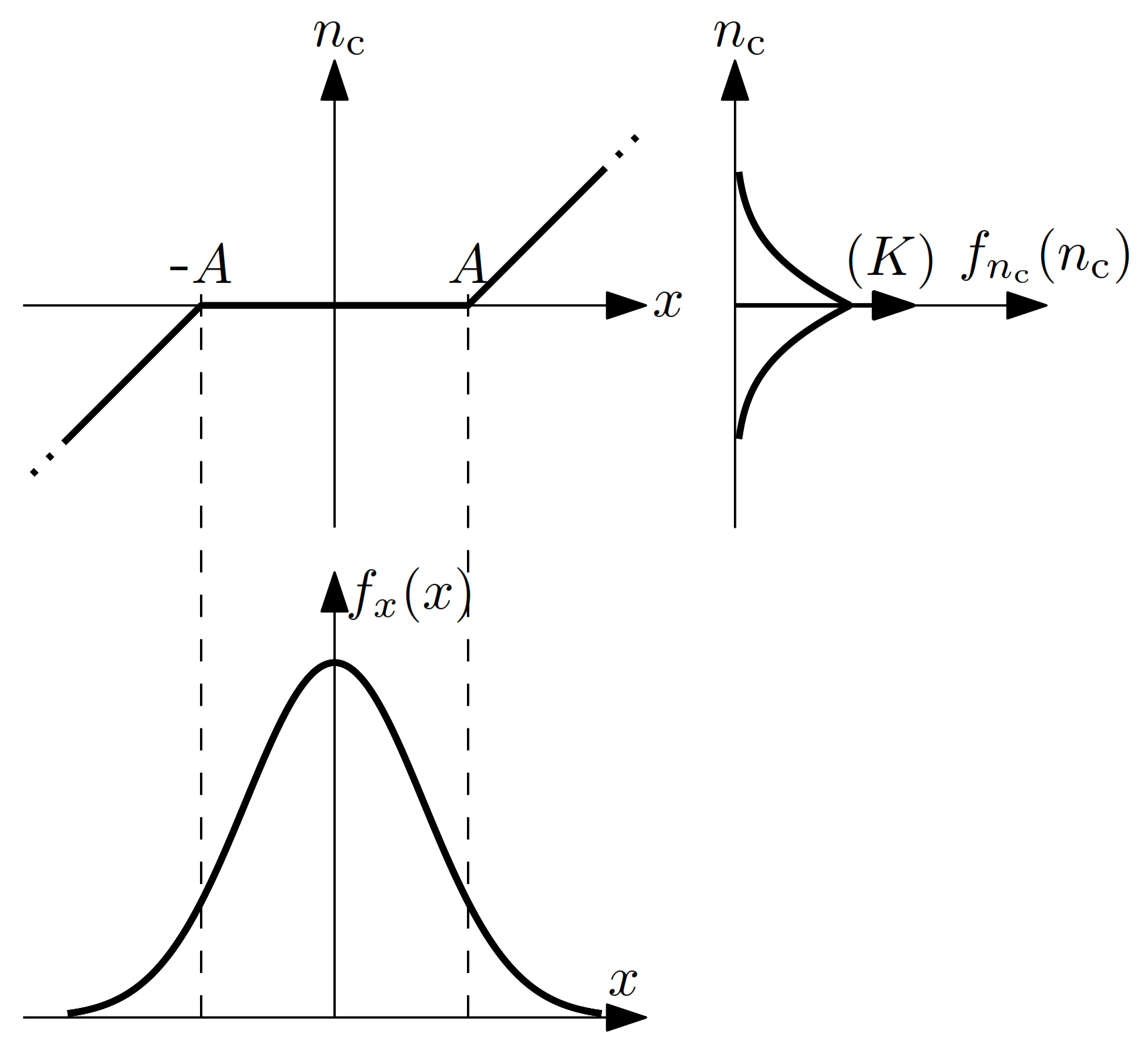
3.1.2. Calculation of the Noise Variance
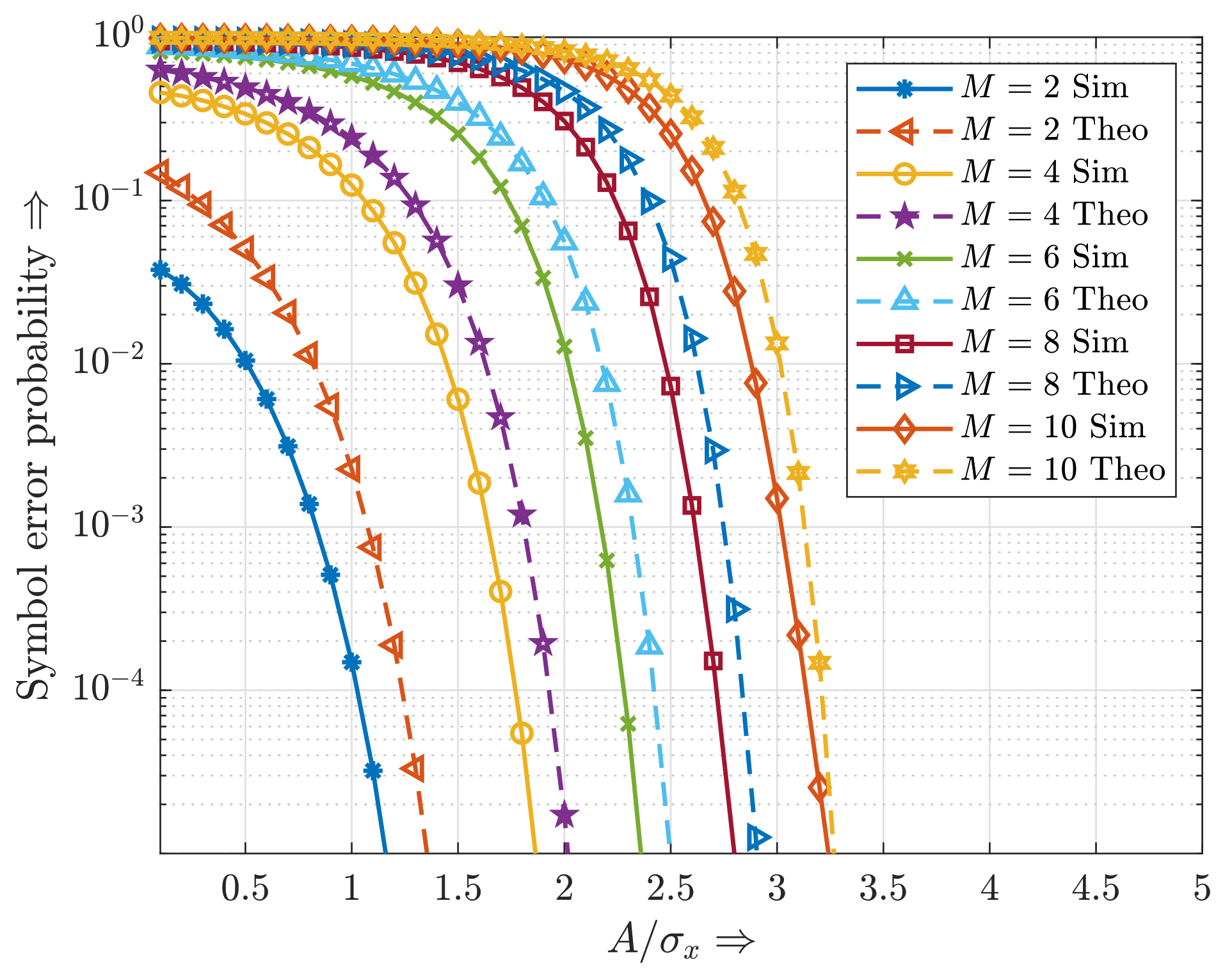
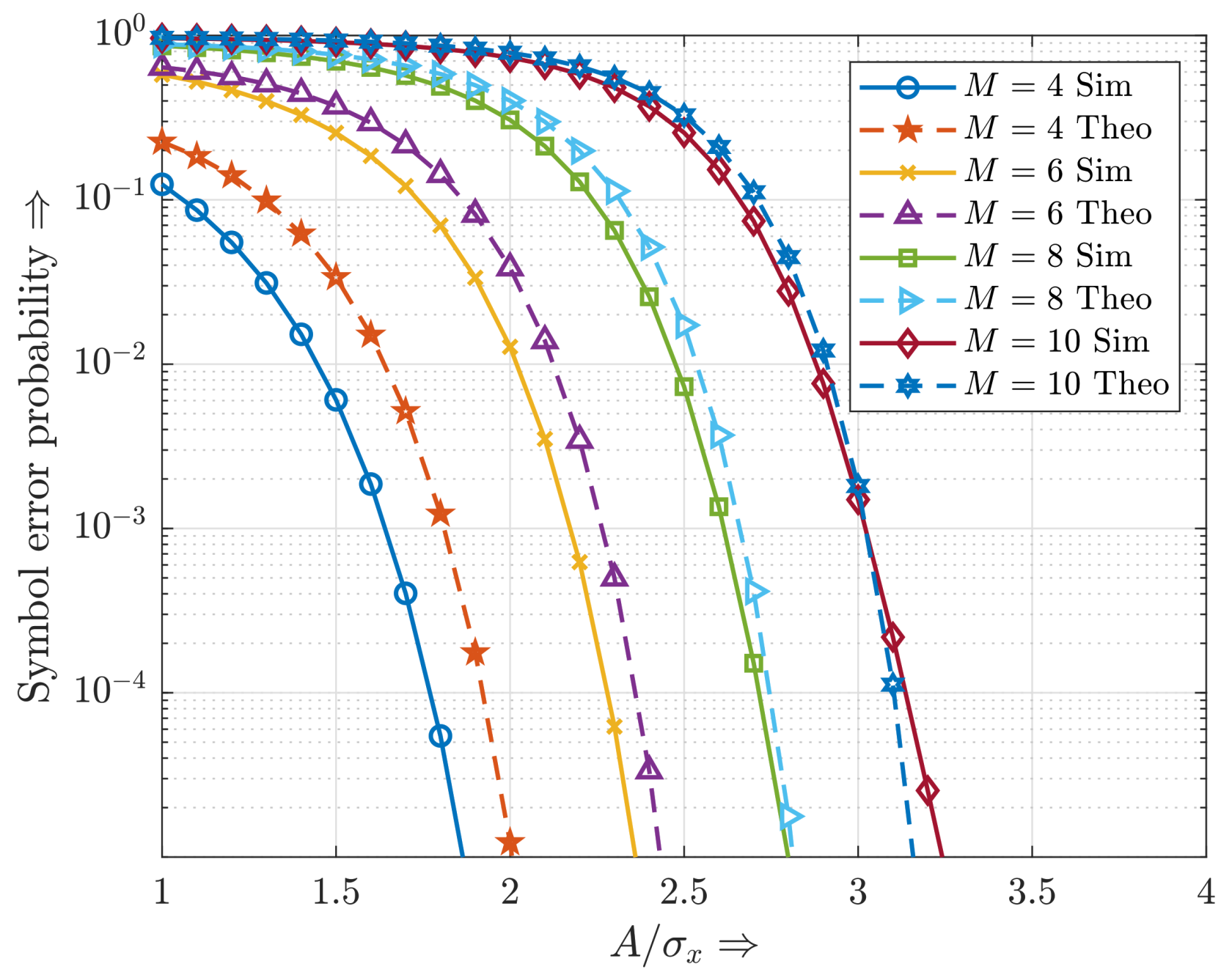
3.2. Symbol Error Probability Based on the Bussgang Theorem
4. Power Spectral Density of the Clipping Distortion
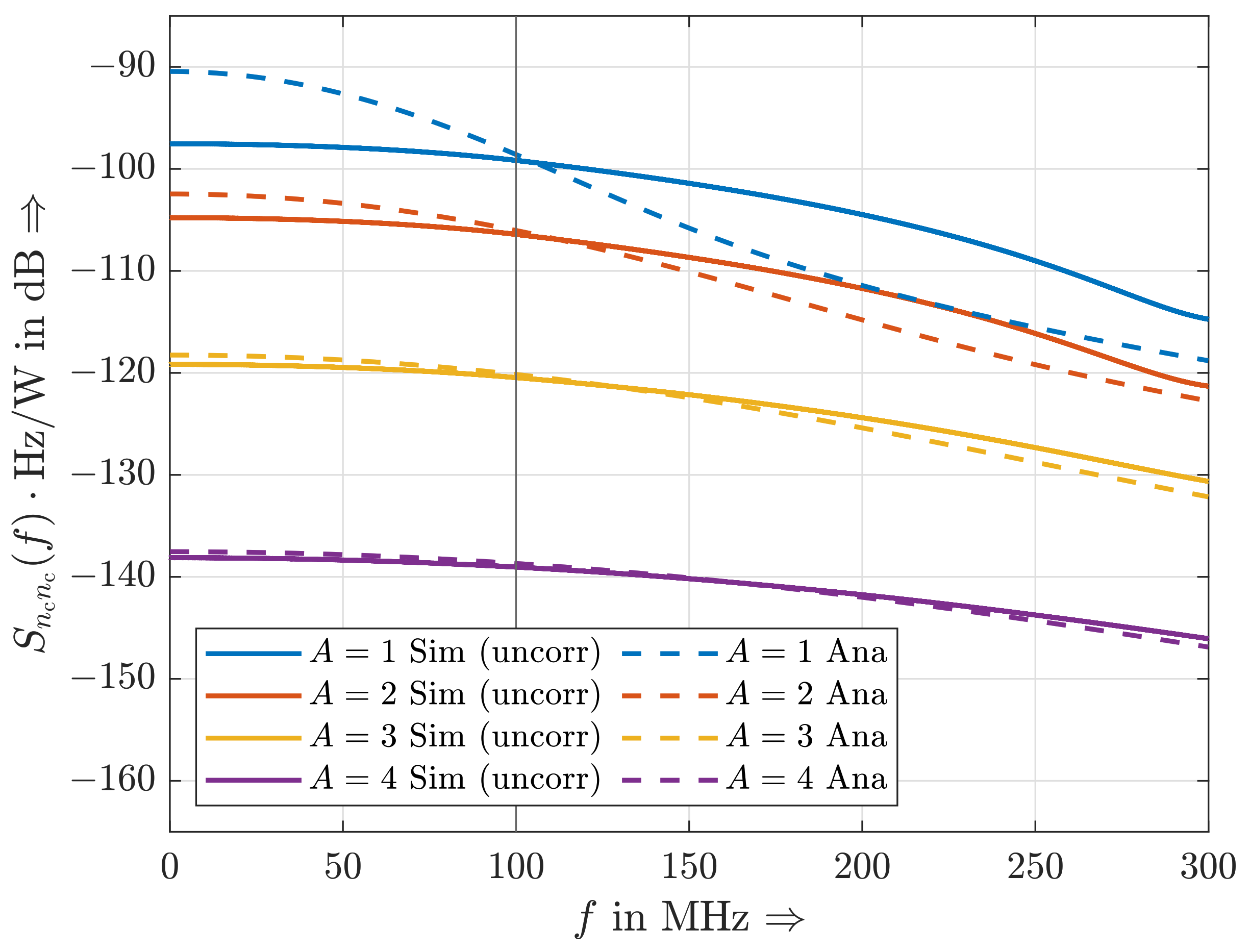
4.1. Analytical Calculation of the Power Spectral Density of Clipping Noise
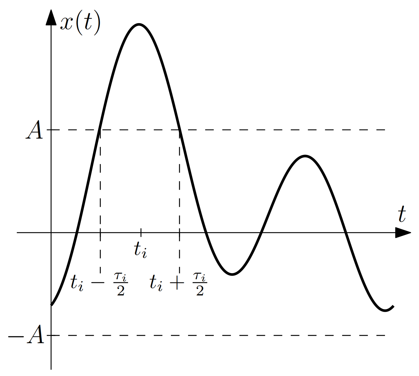
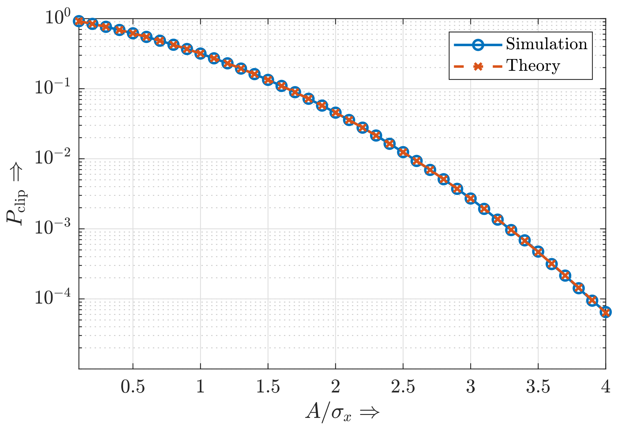
4.1.1. Clipping Level Crossing
4.1.2. Duration of an Overshooting
4.1.3. Mathematical Description of an Overshooting
4.1.4. Closed-Form Analytical Expression of the Power Spectral Density
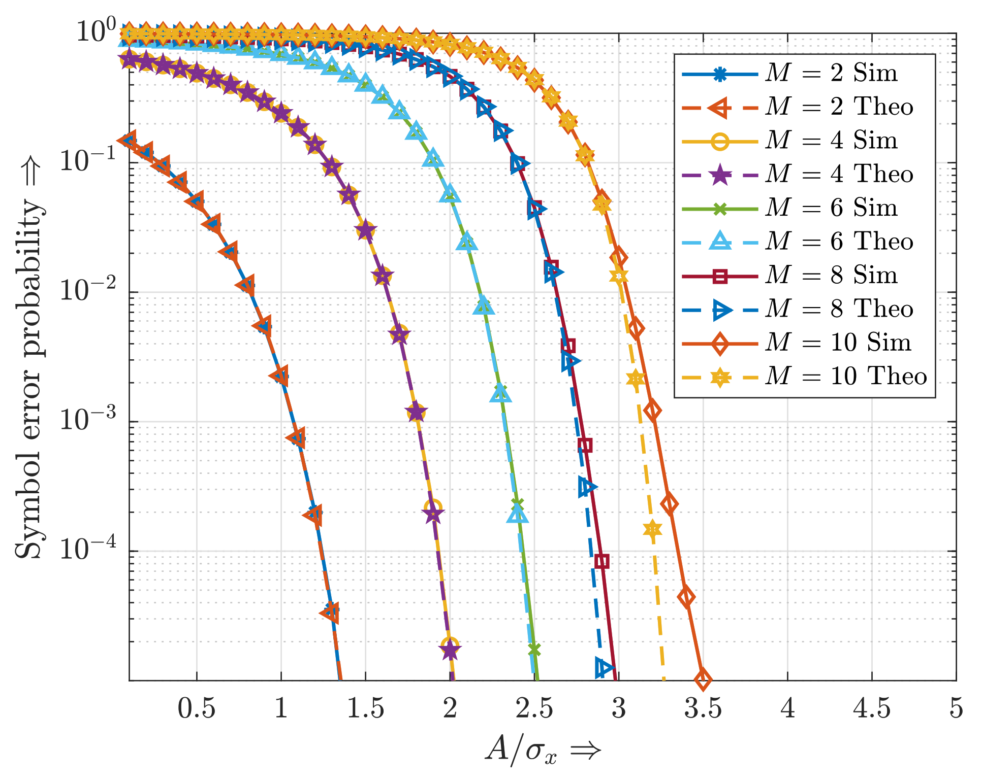
4.2. Symbol Error Probability Based on the Analytical Power Spectral Density of Clipping Noise
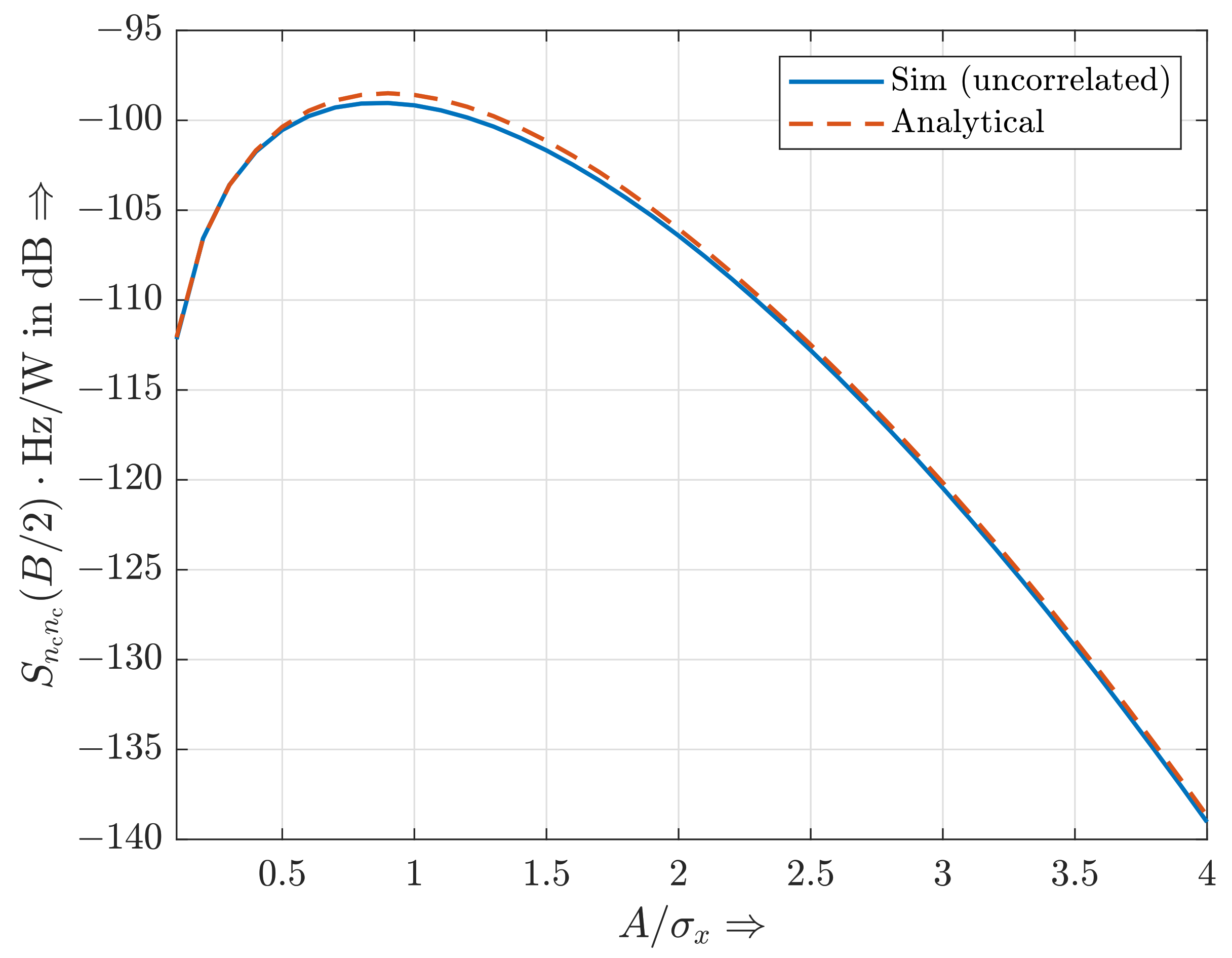
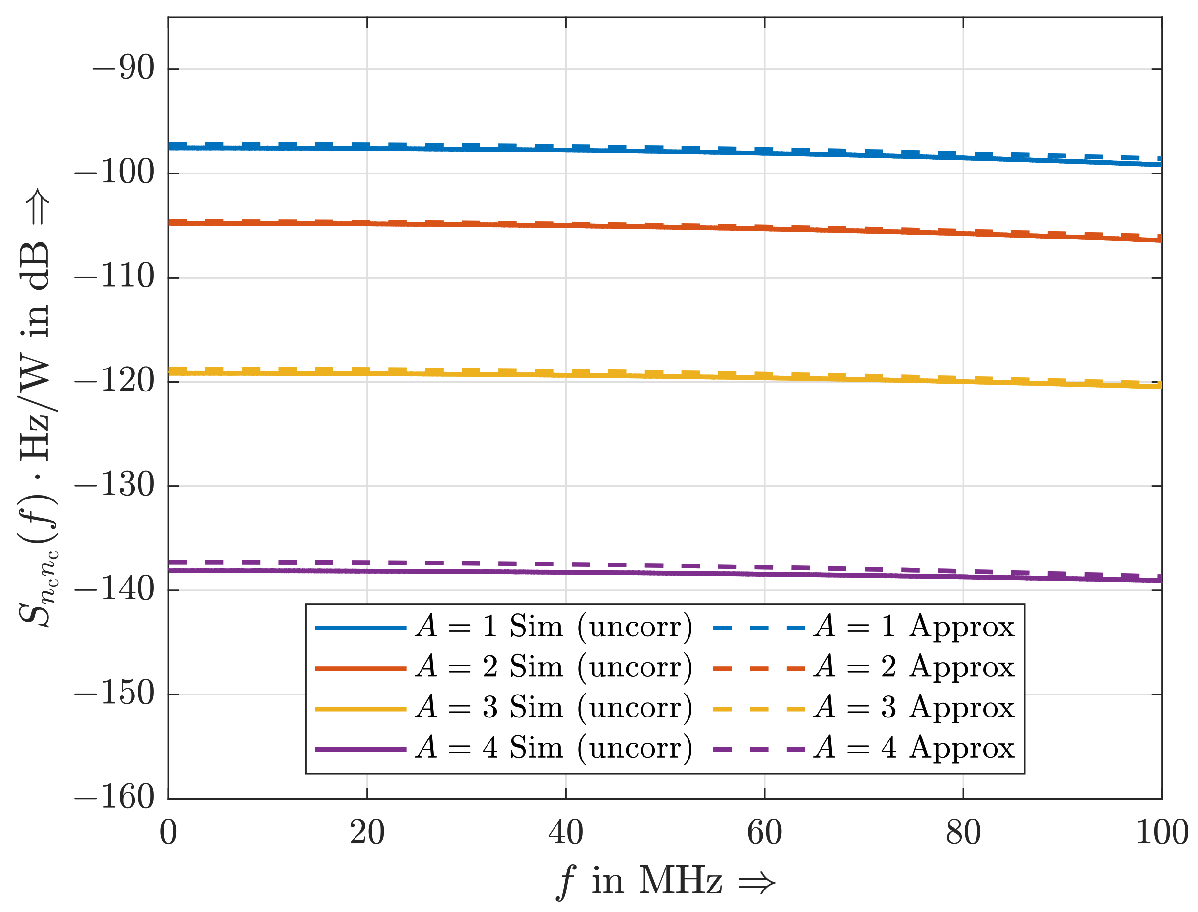
4.3. Approximated Power Spectral Density of Clipping Noise
- The simulated and analytical curves intersect at the corner frequency ;
- The gain from to in dB appears to similar for all A; and
- The shape of the analytical curves in dB inside the transmission bandwidth can be approximated by a quadratic function and does not depend on A as well.
4.4. Symbol Error Probability Based on the Approximated Power Spectral Density of Uncorrelated Clipping Noise
5. Conclusions
Author Contributions
Funding
Acknowledgments
Conflicts of Interest
Appendix A. Detailed Calculations
Appendix A.1
Appendix A.2
References
- Afgani, M.; Haas, H.; Elgala, H.; Knipp, D. Visible light communication using OFDM. In Proceedings of the 2nd International Conference on Testbeds and Research Infrastructures for the Development of Networks and Communities, Barcelona, Spain, 1–3 March 2006. [Google Scholar]
- Czylwik, A. Kanalkapazität intensitätsmodulierter optischer Übertragungssysteme mit Direktempfängern. Frequenz 1996, 50, 60–68. [Google Scholar] [CrossRef]
- Kahn, J.M.; Barry, J.R. Wireless infrared communications. Proc. IEEE 1997, 82, 265–298. [Google Scholar] [CrossRef] [Green Version]
- Armstrong, J. OFDM for Optical Communications. J. Light. Technol. 2009, 27, 189–204. [Google Scholar] [CrossRef]
- Huang, Y.; Liu, Y.; Shi, L.; Shi, D.; Zhang, X.; Aglzim, E.-H.; Zheng, J. On improving the accuracy of Visible Light Positioning system with SLM-based PAPR reduction schemes. In Proceedings of the 2020 IEEE International Symposium on Broadband Multimedia Systems and Broadcasting (BMSB), Paris, France, 27–29 October 2020. [Google Scholar]
- Offiong, F.B.; Sinanovic, S.; Popoola, W.O. On PAPR Reduction in Pilot-Assisted Optical OFDM Communication Systems. IEEE Access 2017, 5, 8916–8929. [Google Scholar] [CrossRef]
- Dimitrov, S.; Sinanovic, S.; Haas, H. Clipping Noise in OFDM-Based Optical Wireless Communication Systems. IEEE Trans. Commun. 2012, 60, 1072–1081. [Google Scholar] [CrossRef]
- Randel, S.; Breyer, F.; Lee, S.C.J.; Walewski, J.W. Advanced Modulation Schemes for Short-Range Optical Communications. IEEE J. Sel. Top. Quantum Electron. 2010, 16, 1280–1289. [Google Scholar] [CrossRef]
- Tsonev, D.; Sinanovic, S.; Haas, H. Complete Modeling of Nonlinear Distortion in OFDM-Based Optical Wireless Communication. J. Light. Technol. 2013, 31, 3064–3076. [Google Scholar] [CrossRef]
- Mazahir, S.; Chaaban, A.; Elgala, H.; Alouini, M.-S. Achievable Rates of Multi-Carrier Modulation Schemes for Bandlimited IM/DD Systems. IEEE Trans. Wirel. Commun. 2019, 18, 1957–1973. [Google Scholar] [CrossRef]
- Jiang, Z.; Gong, C.; Xu, Z. Clipping Noise and Power Allocation for OFDM-Based Optical Wireless Communication Using Photon Detection. IEEE Wirel. Commun. Lett. 2018, 8, 237–240. [Google Scholar] [CrossRef]
- Wang, T.Q.; Li, H.; Huang, X. Analysis and Mitigation of Clipping Noise in Layered ACO-OFDM Based Visible Light Communication Systems. IEEE Trans. Commun. 2019, 67, 564–577. [Google Scholar] [CrossRef]
- Bussgang, J.J. Crosscorrelation Functions of Amplitude-Distorted Gaussian Signals; Tech. Rep. 216; Research Laboratory of Electronics, Massachusetts Institute of Technology: Cambridge, MA, USA, 1952. [Google Scholar]
- Mazo, J.E. Asymptotic distortion spectrum of clipped, DC-biased, Gaussian noise. IEEE Trans. Commun. 1992, 40, 1339–1344. [Google Scholar] [CrossRef]
- Rice, S.O. Distribution of the Duration of Fades in Radio Transmission: Gaussian Noise Model. Bell Syst. Tech. J. 1958, 37, 581–635. [Google Scholar] [CrossRef]
- Czylwik, A. Error Probability due to Clipping in Subcarrier Multiplexed Fiber-Optic Transmission Systems. Frequenz 2000, 54, 52–57. [Google Scholar] [CrossRef]
- Elgala, H.; Mesleh, R.; Haas, H. Practical considerations for indoor wireless optical system implementation using OFDM. In Proceedings of the 10th International Conference on Telecommunications, Zagreb, Croatia, 8–10 June 2009. [Google Scholar]
- Ohm, J.-R.; Lüke, H.D. Mehrpegelübertragung. In Signalübertragung, 12. Auflage; Springer: Berlin/Heidelberg, Germany, 2014; pp. 309–313. [Google Scholar]
- Papoulis, A. The concept of a random variable. In Probability, Random Variables and Stochastic Processes, 4th ed.; McGraw-Hill Higher Education: New York, NY, USA, 2002; pp. 94–95. [Google Scholar]
- Proakis, J.G. Probability of Error for QAM. In Digital Communications, 4th ed.; McGraw-Hill Higher Education: New York, NY, USA, 2001; pp. 276–279. [Google Scholar]


| Parameter | Shortcut | Value |
|---|---|---|
| Subcarriers | N | 8192 |
| Bandwidth | B | |
| Oversampling factor | – | 50 |
| Modulation order | M | 2:2:10 |
| Signal power | 1 | |
| Clipping level | A | 0.1:0.1:4 |
Publisher’s Note: MDPI stays neutral with regard to jurisdictional claims in published maps and institutional affiliations. |
© 2021 by the authors. Licensee MDPI, Basel, Switzerland. This article is an open access article distributed under the terms and conditions of the Creative Commons Attribution (CC BY) license (https://creativecommons.org/licenses/by/4.0/).
Share and Cite
Frömming, A.; Häring, L.; Czylwik, A. Spectral Properties of Clipping Noise. Mathematics 2021, 9, 2592. https://doi.org/10.3390/math9202592
Frömming A, Häring L, Czylwik A. Spectral Properties of Clipping Noise. Mathematics. 2021; 9(20):2592. https://doi.org/10.3390/math9202592
Chicago/Turabian StyleFrömming, Alexander, Lars Häring, and Andreas Czylwik. 2021. "Spectral Properties of Clipping Noise" Mathematics 9, no. 20: 2592. https://doi.org/10.3390/math9202592
APA StyleFrömming, A., Häring, L., & Czylwik, A. (2021). Spectral Properties of Clipping Noise. Mathematics, 9(20), 2592. https://doi.org/10.3390/math9202592