
Discovering Geometric Inequalities: The Concourse of GeoGebra Discovery, Dynamic Coloring and Maple Tools


Abstract
1. Introduction
2. The GeoGebra Automated Reasoning Tools
- (i)
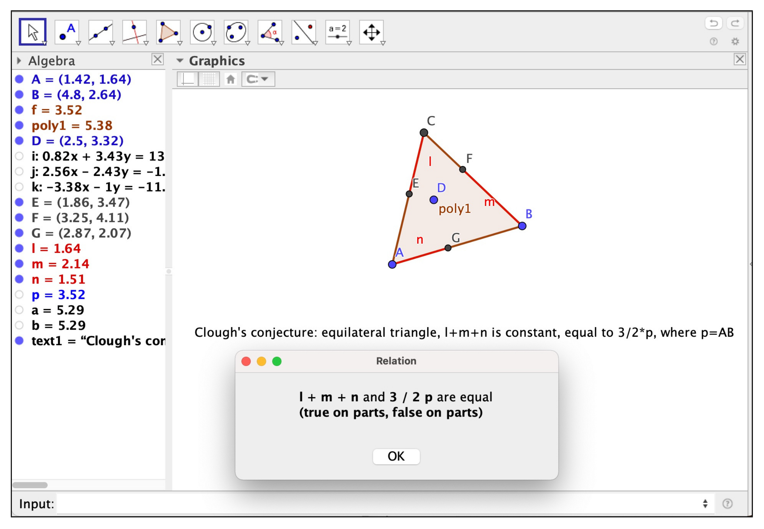
- The use of complex versus real geometry tools: Points in the Euclidean plane have real coordinates, while the algebraic algorithms used within this framework are designed for algebraically closed fields. Therefore, when we state that we are including points in with complex coordinates, which is more than what we actually need. We could be missing valid theses which hold for all real points in , but not on the whole complex variety (see [17,18]). For example, let us consider the following statement, usually called Clough’s conjecture [19], namely, the equality of
- -
- the sum of segments , , and , where are the feet of the perpendiculars to the sides of an equilateral triangle from an arbitrary point D,
- -
- and , where p is the length of side , i.e., is half the perimeter of the equilateral triangle .
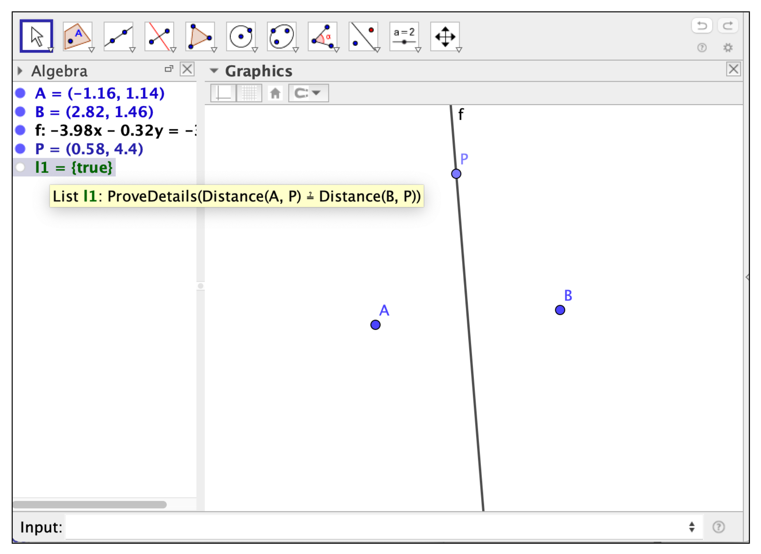
See [20] for detailed synthetic and algebraic proofs. Now, the algorithms we have implemented in GeoGebra, if asked about the Relation between and , proceed, first, checking the numerically approximate equality of both quantities and, if it holds, starting a symbolic protocol by considering the ideal generated by all the polynomial equations describing the hypotheses. We emphasize here the terms polynomial equations, because all the lengths are described by expressing as the sum of the squares of the differences of the coordinates of the extremes of the corresponding segments, say, , etc. There are neither square roots nor choice of positive signs for defining , as this approach would require real algebraic geometry methods. Thus, our hypotheses ideal includes much more cases (in the complex geometry context) than intuitively expected, and the thesis , holds only on some of them (for example, on those cases where are positive).Accordingly, GeoGebra Discovery declares that the formulated statement is “true on parts, false on parts”, see Figure 2. This means that the underlying algorithm detects, without having to compute a primary decomposition of the involved hypotheses ideal, that the statement holds true on some components and is false on some others, see item iii) below.On the other hand, asking directly for the proof of Clough’s statement, see Figure 3, an affirmative answer is obtained, together with a list (too long in this case to be fully displayed in the Figure) of construction instances that should be avoided for the truth of the statement: degenerate cases such as when the triangle collapses and, also, variants of the thesis statement that hold just on the primary components of the hypotheses where the given thesis is false.This is related to the possibility, in this case, to modify the thesis so that it collects all possible sign choices for , by multiplying by all possible variants of such formula, changing signs for , such as , , etc. See [21] for a detailed study of this way of understanding real statements in a complex geometry context.Of course, the reason for choosing a complex algebraic geometry approach for GeoGebra automated reasoning tools is because algorithms based on complex geometry are generally much more efficient than their real counterparts, and this aspect is of special relevance for the implementation of GARTs in software with educational purposes. - (ii)
- Non-degeneracy conditions: In Geometry statements, whenever we mention objects such as line segments, polygons, circles..., we implicitly assume certain conditions on the points that are used to define those figures and render a theorem as true. As an example, in a theorem on triangles we always assume that its vertices are non-collinear points of the plane. These conditions are not easy to interpret by the GATPs and require special care when dealing with them. The problem of non-degeneracy conditions, which depends upon the choice of independent variables in the construction, the way the construction itself is carried out, or the interpretation we can give to what a degenerate construction is, has been studied extensively in the literature and the reader is referred to [12,22,23,24,25] or [26] to gain a better understanding of the intricacies surrounding it.
- (iii)
- True on parts, false on parts statements: As already explained in item i), quite often the hypothesis variety that is obtained from the algebraization process (via complex geometry algorithms which avoid the computationally costly decomposition of the hypothesis variety into irreducible components) can have irreducible, non-degenerate components of maximal dimension, such that the thesis holds on some of the components, while not on others. This situation was thoroughly treated in [27], and gave rise to a new category of true on parts, false on parts geometric statements.
- Relation(<list of objects>): This higher level command performs two distinct operations: In the first place it proceeds to make a numerical comparison of the objects, and outputs an answer concerning geometric properties such as equality/inequality, parallelism, collinearity, concurrency, etc. Together with this numerical output, the user finds a “More...” button that, when clicked, gives way to a deeper, symbolic analysis of the numerical result previously obtained, resorting to the commands that mention below and proving or rejecting its truthfulness. See Figure 2.
- Prove(<Boolean Expression>): This command is the basic symbolic automatic theorem prover in GeoGebra, and its output can be (generally) true, (generally) false or undefined/? (when GeoGebra cannot decide the question). In order to introduce easily the Boolean expressions of geometric nature, GeoGebra offers a number of different commands such as AreParallel(<line>,<line>), AreCollinear(<Point>,<Point>, <Point>), AreConcyclic(<Point>,<Point>,<Point>,<Point>), etc.
- ProveDetails(<Boolean Expression>): Improved version of the previous command, offering as output more information on degeneracy conditions whenever they are easy to translate into a simple statement. See Figure 3.
- LocusEquation(<Arguments>): This command offers the possibility of finding the algebraic equation for a geometric locus, obtained also by symbolic means. Besides, the command shows on the graphic window the curve corresponding to the equation. Among the several options for choosing the arguments, one which will be useful later to our purposes is LocusEquation(<Boolean expression>, <Point>); this command will find the equation for the locus of points satisfying the given Boolean expression.
- Discover(<Point>): This command, one of the latest additions in GeoGebra Discovery, provides as output from a geometric construction a whole set of geometric statements concerning properties about the lines, segments and other geometric elements related to the point provided as argument. The inner workings of the command follow the idea exposed in Strategies 1 and 3 above.
3. New Tools in GeoGebra Discovery: Handling Geometric Inequalities
- If j is odd, then
- If j is even, then
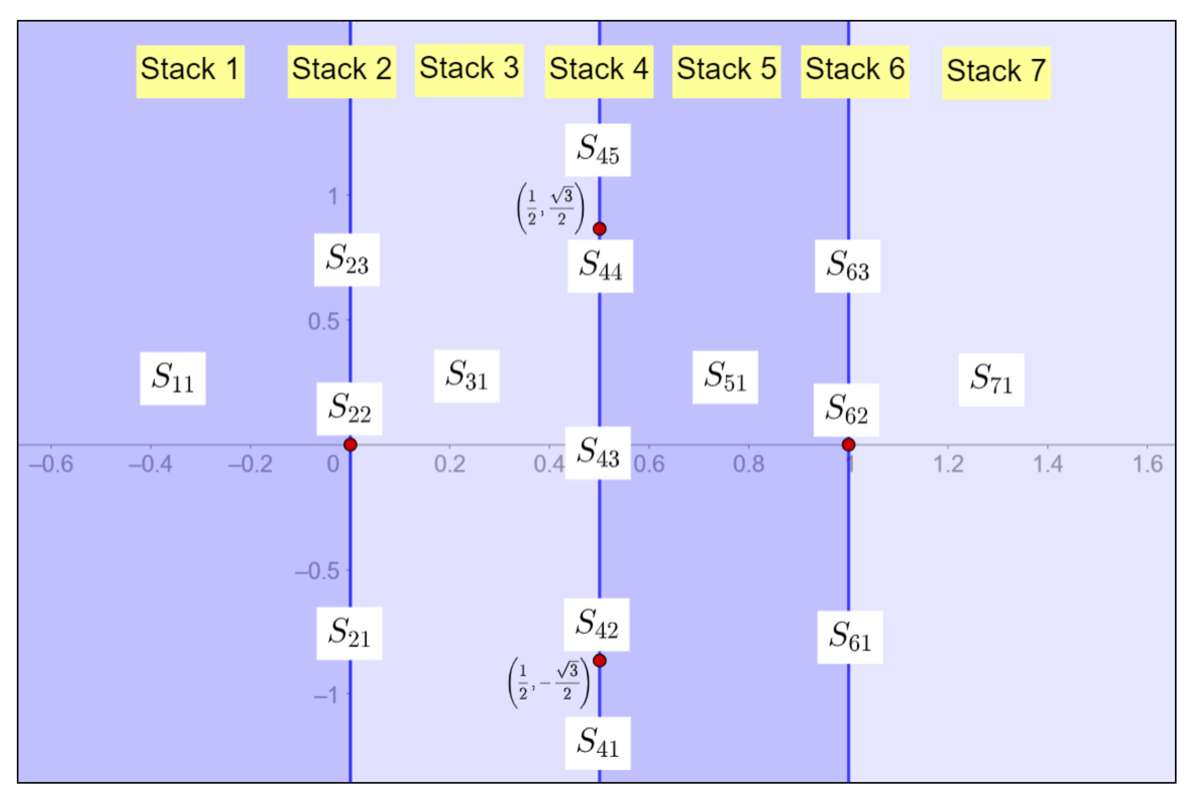
- For , a CAD of is a finite partition of the real line in k points and the open intervals which constitute their complement (it can be viewed as a stack over a point). A point is called a 0-cell and an open interval a 1-cell of the CAD.
- For , a CAD of is a partition of in stacks , whose elements are semialgebraic sets, and such that the collection , is a CAD of (here we have renamed and reindexed the elements of the —dimensional CAD to avoid accumulation of subindices). If is a k-cell, then is either a -cell (if j is odd) or a k-cell (if j is even). Besides, and, by the recursive nature of the construction, the collection of sets (with repeated elements) forms a CAD of .
- Compare(<Expression, Expression>): This command performs a sequence of tasks that can be briefly described as follows (see [40]):
- The first two points of the construction are identified with (0,0) and (1,0). This reduces the number of variables required, and avoids some degenerate configurations.
- By using only the equalities defining the hypothesis, there is a first trial to check for an equality relation between the input expressions. This is handled by the Giac CAS embedded in GeoGebra.
- If equality relations are not found, the set of equations in the hypothesis is processed, eliminating unnecessary variables and generating a quantified formula.
- Now, via the Tarski/QEPCAD B software, this quantified formula is converted into a quantifier-free formula, by means of a CAD algorithm that outputs an inequality for the quotient of the input expressions.
- This inequality is translated and displayed into a simple form, easy to understand by the user.
See Figure 5 for an example of the performance of the Compare command regarding the statement of Proposition 1. - Relation(<list of objects>): As mentioned before, this higher level command performs two distinct operations ([28]): first, proceeds to make a numerical comparison of the objects, and outputs an answer concerning geometric properties, including—this is the more recent improvement—inequalities, etc. Then the user finds a “More...” button that, if clicked, starts a deeper, symbolic analysis of the numerical result previously obtained, proving or rejecting its truthfulness. A detailed example is developed in Section 5, and shown in Figures 10 and 11.
4. Visualization of Real Curves and the Dynamic Color Scanning Method
- Red: c/s
- Green: 1-abs(s-c)
- Blue: s/c,
- The periodic patterns that frequently arise in form of concentric rings of similar colors are due to the periodic behavior of the dynamic colors when the values introduced in the RGB channels move outside the range, as previously mentioned (see Figure 9b).
- A way to restrict the values for the dynamic color channels in the range is obtained by using exponential expressions of the form
- Red: e^(-abs(f(P)))
- Green: e^(-abs(g(P)))
- Blue: e^(-abs(h(P))),
so that only when simultaneously the functions , depending on point P, are equal to 0 the white color will be assigned to P. In our example, by assigning to the color channels the values- Red: e^(-abs(1-c/s))
- Green: e^(-abs(s-c))
- Blue: e^(-abs(1-s/c)),
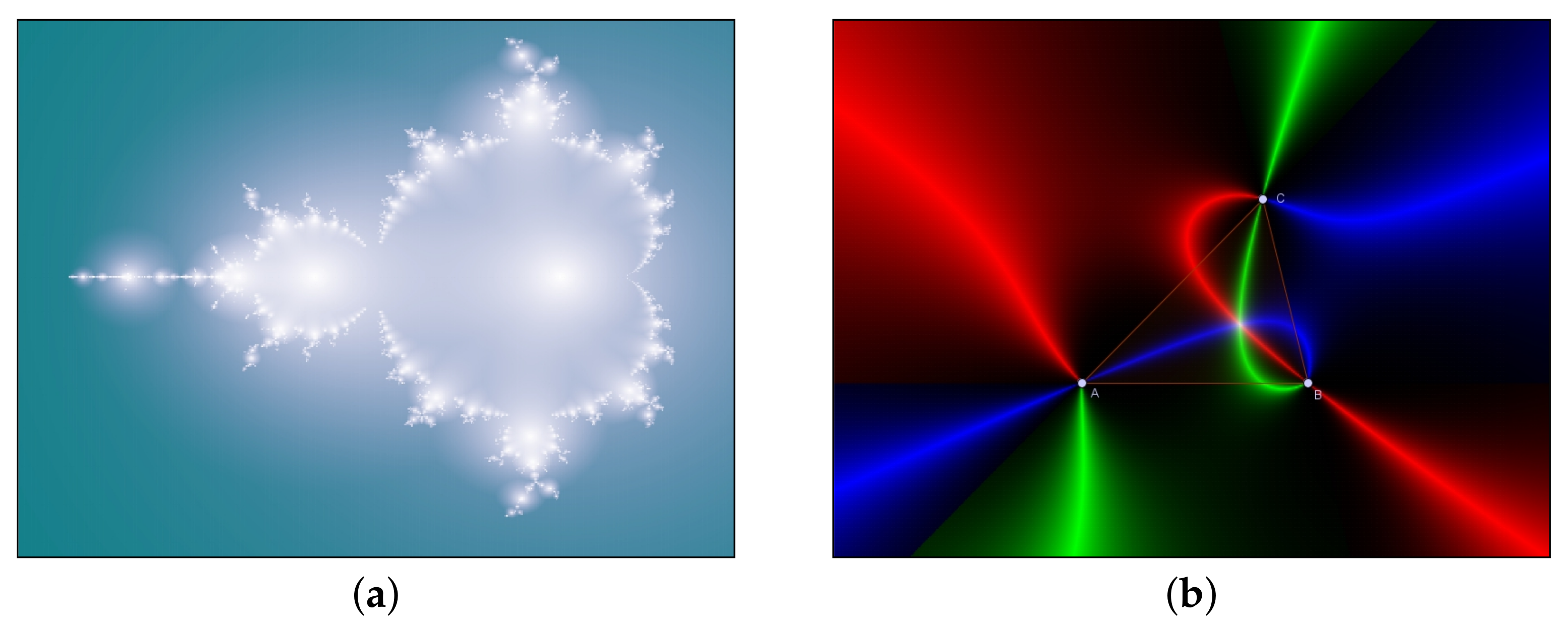
we obtain Figure 9c.Besides, if we substitute in a given RGB channel, for instance the red one, the expression in the exponent by , where k is a convenient positive constant, we get the mantissa of , which drops abruptly to zero when crosses integer values, producing distinct lines because of the sudden color change in the red channel. This trick leads to the appearance of level curves connecting points P with the same value, which will be more densely distributed by choosing a greater value for the constant k. We will make use of this technique later in Section 6.1. - Since we have three different channels that can hold independent values, by playing wisely with them, we have at our disposal up to three different properties to visualize in our scanning method. An illustration of how to take advantage of this feature is shown in Figure 8b, where an investigation on the Fermat’s Point is carried out (see the section on “Escáner del Punto Fermat” in [44], for details on the construction).
- Set a rectangular region to be scanned. Let us say it has as upper left corner the point , and dimensions .
- Shrink the size of the radius for the point P to its minimum size.
- Create a slider t that will be used as the x-coordinate of P, and runs from to .
- Set the coordinates of P to and rename the point to . This trick allows us to automatically assign the point P to the cell of the GeoGebra spreadsheet. Now we can create a list of points , , by taking advantage of the spreadsheet features, starting first by adding the point , with the same properties as A1, and dragging downwards (as it is usually done when working with spreadsheets) the cell A2. This column of points (all of them inheriting the properties we set up for ) translates in the graphic window into a scanning vertical segment, which will sweep the region as the slider t runs through its defined range. A recommended value for is in order to obtain a good quality of the scanning image. Therefore, for covering our rectangular region of height h we should create around h points.
5. A Case Study: Relation between the Perimeter and Circumradius of a Triangle
6. Combining Visual and Symbolic Strategies to Overcome Difficulties
6.1. The Visual Approach Using the Dynamic Color Scanning Method
- Red: e^(-(abs(k Bi)-floor(abs(k Bi))))
- Green: e^(-abs(Bi))
- Blue: e^(-(abs(Bi)-floor(abs(Bi)))),
6.2. The Symbolic Approach Using Maple Commands
- >
- with(RegularChains):with(ChainTools):with(SemiAlgebraicSetTools):R:=PolynomialRing([y,x])cad:=CylindricalAlgebraicDecompose(P,R,method = recursive,output=piecewise)
- >
- restart:with(PolynomialIdeals):Hypo:=PolynomialIdeal(u-(1/2),(x-1)*(u-((x+1)/2))+y*(v-(y/2)),h^2-(x-u)^2-(y-v)^2,a^2-(x-1)^2-y^2,b^2-x^2-y^2,c^2-1, variables={x,y,u,v,h,a,b,c});
- >
- HilbertDimension(Hypo);EliminationIdeal(Hypo,{x,y});
- >
- T:=PolynomialIdeal(u-(1/2),(x-1)*(u-((x+1)/2))+y*(v-(y/2)),h^2-(x-u)^2-(y-v)^2,a^2-(x-1)^2-y^2,b^2-x^2-y^2,c^2-1,r^2-3,a+b+c-3*r*h,variables={x,y,u,v,h,a,b,c,r});HilbertDimension(T);
- >
- P:=EliminationIdeal(T,{x,y});
- >
- with(algcurves): plot_real_curve(P(x,y),x,y);
- Step 1:
- Check that for has real solutions in y, and determine them all.
- Step 2:
- Check that for has not real solutions in y.
- Step 1:
- We first set and compute , factorizing the result.
- >
- simplify(subs(x=0,P(x,y))); factor(%);
- >
- sturmseq(297*y^4 + 432*y^3 + 658*y^2 + 432*y + 297,y);sturm(%,y, -infinity, infinity);
- >
- simplify(subs(x=1,P(x,y)));
- >
- simplify(subs(x=1/2,P(x,y)));
- >
- sturmseq(1936*y^4 + 744*y^2 + 81,y);sturm(%,y, -infinity, infinity);
- >
- sturmseq(432*y^4 + 152*y^2 + 27,y);sturm(%,y, -infinity, infinity);
- Step 1:
- We start by considering again the polynomial , but now displayed as a polynomial in , that is, as a polynomial in the variable y with coefficients in the domain :
- >
- P(y):=collect(P(x,y),y);
- >
- F(x):=discrim(P(y),y);
- >
- factor(F_1);factor(F_2);
- >
- sturmseq(221709312*x^10 - 1108546560*x^9 + 5547202304*x^8−15537529856*x^7 + 23360155968*x^6 - 20355008960*x^5+10731606224*x^4 - 3448222560*x^3 + 658900764*x^2−70266636*x + 3485889,x);sturm(%,x,-infinity, infinity);
- >
- subs(x=-1,P(y)); sturmseq(%,y):sturm(%,y,-infinity, infinity);
- >
- subs(x=1/3,P(y)); sturmseq(%,y):sturm(%,y,-infinity,infinity);
- >
- subs(x=2/3,P(y)); sturmseq(%,y):sturm(%,y,-infinity,infinity);
- >
- subs(x=2,P(y)); sturmseq(%,y):sturm(%,y,-infinity,infinity);
7. Conclusions and Further Research
- (i)
- perform straightforwardly a dynamic color scanning, avoiding the setup process which is needed at present and improving its performance;
- (ii)
- utilize the Giac and Tarski/QEPCAD embedded systems to increase the power of the GART’s tools present in GeoGebra, rendering unnecessary to make use of external software to visualize and study certain geometric problems (see for instance [53]) which can involve equalities or inequalities in their formulation.
Author Contributions
Funding
Acknowledgments
Conflicts of Interest
Abbreviations
| CAD | Cylindric Algebraic Decomposition |
| CAS | Computer Algebra System |
| DGS | Dynamic Geometry Software |
| GART | Geometry Automated Reasoning Tool |
| GATP | Geometry Automated Theorem Prover |
References
- Wu, W.T. On the decision problem and the mechanization of theorem-proving in elementary geometry. Sci. Sin. 1978, 21, 159–172, Reprinted in: Automated Theorem Proving: After 25 Years; Bledsoe, W.W., Loveland, D.W., Eds.; Contemporary Mathematics, 29; AMS: Providence, RI, USA, 1984; pp. 213–234. [Google Scholar]
- Quaresma, P. Thousands of Geometric problems for geometric Theorem Provers (TGTP). In Automated Deduction in Geometry, 8th International Workshop, ADG 2010; Schreck, P., Narboux, J., Richter-Gebert, J., Eds.; LNAI 6877; Springer: Berlin/Heidelberg, Germany, 2011; pp. 169–181. [Google Scholar]
- Chou, S.C. An Introduction to Wu’s Method for Mechanical Theorem Proving in Geometry. J. Autom. Reason. 1988, 4, 237–267. [Google Scholar] [CrossRef]
- Buchberger, B. Introduction to Gröbner Bases. In Gröbner Bases and Applications; Buchberger, B., Winkler, F., Eds.; LMSLN 251; Cambridge University Press: Cambridge, UK, 1998; pp. 3–31. [Google Scholar]
- Kapur, D. Using Gröbner bases to reason about geometry problems. J. Symb. Comput. 1986, 2, 399–408. [Google Scholar] [CrossRef]
- About GeoGebra. Available online: https://www.geogebra.org/m/pR5DME5S#material/uy93nfzr (accessed on 21 August 2021).
- Cevikbas, M.; Kaiser, G. A Systematic Review on Task Design in Dynamic and Interactive Mathematics Learning Environments (DIMLEs). Mathematics 2021, 9, 399. [Google Scholar] [CrossRef]
- Ondes, R.N. Research trends in dynamic geometry software: A content analysis from 2005 to 2021. World J. Educ. Technol. Curr. Issues 2021, 13, 236–260. [Google Scholar] [CrossRef]
- Kovács, Z.; Montag, A.; Vajda, R. On Euler’s inequality and automated reasoning with dynamic geometry. arXiv 2020, arXiv:1708.02993. [Google Scholar]
- Bottema, O.; Djordjević, R.Ž.; Janić, R.R.; Mitrinović, D.S.; Vasić, P.M. Geometric Inequalities, 1st ed.; Wolters-Noordhoff Publishing: Groningen, Germany, 1969. [Google Scholar]
- Hohenwarter, M.; Kovács, Z.; Recio, T. Using GeoGebra automated reasoning tools to explore geometric statements and conjectures. In Proof Technology in Mathematics Research and Teaching; Hanna, G., de Villiers, M., Reid, D., Eds.; Mathematics Education in the Digital Era 14; Springer: Berlin/Heidelberg, Germany, 2019; pp. 215–236. [Google Scholar]
- Recio, T.; Vélez, M.P. Automatic Discovery of Theorems in Elementary Geometry. J. Autom. Reason. 1999, 23, 63–82. [Google Scholar] [CrossRef]
- Botana, F.; Kovács, Z.; Recio, T. A Mechanical Geometer. Math.Comput. Sci. 2020. [Google Scholar] [CrossRef]
- De Graeve, R.; Parisse, B. Giac/Xcas (v. 1.7.0). 2021. Available online: https://www-fourier.ujf-grenoble.fr/~parisse/giac.html (accessed on 29 July 2021).
- Kovács, Z.; Parisse, B. Giac and GeoGebra—Improved Gröbner Basis Computations. In Computer Algebra and Polynomials; Gutiérrez, J., Schicho, J., Weimann, M., Eds.; Lecture Notes in Computer Science; Springer: Berlin/Heidelberg, Germany, 2015; pp. 12–138. [Google Scholar]
- Cox, D.A.; Little, J.; O’Shea, D. Ideals, Varieties, and Algorithms: An Introduction to Computational Algebraic Geometry and Commutative Algebra, 3rd ed.; Springer: Cham, Germany, 2015. [Google Scholar]
- Conti, P.; Traverso, C. Algebraic and semialgebraic proofs: Methods and paradoxes. In Proc. 3rd International Workshop on Automated Deduction in Geometry (ADG 2000); Richter-Gebert, J., Wang, D., Eds.; LNAI, 2061; Springer: Berlin/Heidelberg, Germany, 2000; pp. 83–103. [Google Scholar]
- Dolzmann, A.; Sturm, T.; Weispfenning, V. A New Approach for Automatic Theorem Proving in Real Geometry. J. Autom. Reason. 1998, 21, 357–380. [Google Scholar] [CrossRef]
- De Villiers, M. Clough’s conjecture: A Sketchpad investigation. In Proceedings of the 10th Annual National Congress of the Association for Mathematics Education of South Africa; Nieuwoudt, S., Froneman, S., Nkhoma, P., Eds.; AMESA: Potchefstroom, South Africa, 2004; Volume 2, pp. 52–56. [Google Scholar]
- De Villiers, M. An illustration of the explanatory and discovery functions of proof. Pythagoras 2012, 33, 8. [Google Scholar] [CrossRef]
- Kovács, Z.; Recio, T.; Sólyom-Gecse, C. Rewriting input expressions in complex algebraic geometry provers. Ann. Math. Artif. Intell. 2018, 85, 73–87. [Google Scholar] [CrossRef]
- Chou, S.C. Mechanical Geometry Theorem Proving, 1st ed.; D. Reidel Publishing Company: Dordrecht, Holland, 1988. [Google Scholar]
- Kovács, Z.; Recio, T.; Tabera, L.F.; Vélez, M.P. Dealing with Degeneracies in Automated Theorem Proving in Geometry. Mathematics 2021, 9, 1964. [Google Scholar] [CrossRef]
- Kapur, D. A Refutational Approach to Geometry Theorem Proving. Artif. Intell. 1988, 37, 61–93. [Google Scholar] [CrossRef]
- Bulmer, M.; Fearnley-Sander, D.; Stokes, T. The kinds of truth of geometric theorems in automated deduction in geometry. In Proc. 3rd International Workshop on Automated Deduction in Geometry (ADG 2000); Richter-Gebert, J., Wang, D., Eds.; LNAI, 2061; Springer: Berlin/Heidelberg, Germany, 2000; pp. 129–142. [Google Scholar]
- Guan, H.; Rao, Y.S.; Zhang, J.Z.; Cao, S.; Qin, X.L. Method for Processing Graph Degeneracy in Dynamic Geometry Based on Domain Design. J. Comput. Sci. Technol. 2021, 36, 910–921. [Google Scholar] [CrossRef]
- Kovács, Z.; Recio, T.; Vélez, M.P. Detecting truth, just on parts. Rev. MatemáTica Complut. 2019, 32, 451–474. [Google Scholar] [CrossRef]
- Kovács, Z. The Relation Tool in GeoGebra 5. In Proceedings of the 10th International Workshop on Automated Deduction in Geometry (ADG 2014), Coimbra, Portugal, 9–11 July 2014; Botana, F., Quaresma, P., Eds.; Springer: Berlin/Heidelberg, Germany, 2015; pp. 53–71. [Google Scholar]
- Botana, F.; Hohenwarter, M.; Janičić, P.; Petrović, I.; Recio, T.; Weitzhofer, S. Automated Theorem Proving in GeoGebra: Current Achievements. J. Autom. Reason. 2015, 55, 39–59. [Google Scholar] [CrossRef]
- GeoGebra Discovery. Available online: https://github.com/kovzol/geogebra-discovery (accessed on 29 July 2021).
- Bochnak, J.; Coste, M.; Roy, M.F. Real Algebraic Geometry, 1st ed.; Springer: Berlin/Heidelberg, Germany, 1998. [Google Scholar]
- Davenport, J.; Heintz, J. Real quantifier elimination is doubly exponential. J. Symb. Comput. 1988, 5, 29–35. [Google Scholar] [CrossRef]
- Xia, B.; Yang, L.; Hou, X. Automated discovering and proving for geometric inequalities. In ADG’98: Proceedings of the Second International Workshop on Automated Deduction in Geometry, Beijing, China, 1–3 August 1998; Gao, X.-S., Wang, D., Yang, L., Eds.; Springer: Berlin/Heidelberg, Germany, 1998. [Google Scholar]
- Xia, B.; Yang, L. Automated Inequality Proving and Discovering; World Scientific Publishing Company: Hackensack, NJ, USA, 2017. [Google Scholar]
- Yang, L. Recent advances in automated theorem proving on inequalities. J. Comput. Sci. Technol. 1999, 14, 434–446. [Google Scholar] [CrossRef]
- Collins, G.E. Quantifier elimination for real closed fields by cylindrical algebraic decomposition. In Proc. 2nd GI Conference on Automata. Theory and Formal Languages; Brakhage, H., Ed.; Lecture Notes in Computer Science; Springer: Berlin/Heidelberg, Germany, 1975; Volume 33, pp. 134–183. [Google Scholar]
- Chen, C.; Maza, M.M. Quantifier Elimination by Cylindrical Algebraic Decomposition based on Regular Chains. J. Symb. Comput. 2016, 75, 74–93. [Google Scholar] [CrossRef]
- Kovács, Z.; Vajda, R. GeoGebra and the realgeom reasoning tool. In Proceedings of the Fifth International Workshop on Satisfiability Checking and Symbolic Computation, Paris, France, 5 July 2020; Fontaine, P., Korovin, K., Kotsireas, I.S., Rümmer, P., Tourret, S., Eds.; CEUR Workshop Proceedings. RWTH: Aachen, Germany, 2020; Volume 2752, pp. 204–219. [Google Scholar]
- Brown, C.W. QEPCAD. Extended Tarski Formulas. Available online: https://www.usna.edu/Users/cs/wcbrown/qepcad/B/user/ETF.html (accessed on 12 August 2021).
- Brown, C.W.; Kovács, Z.; Vajda, R. Supporting Proving and Discovering Geometric Inequalities in GeoGebra by Using Tarski. In Proceedings of the 13th International Workshop on Automated Deduction in Geometry (ADG2021), Hagenberg, Austria, 15–17 September 2021. [Google Scholar]
- Brown, C.W. An Overview of QEPCAD B: A Tool for Real Quantifier Elimination and Formula Simplification. J. JSSAC 2003, 10, 13–22. [Google Scholar]
- Cheng, J.; Lazard, S.; Peñaranda, L.; Pouget, M.; Rouillier, F.; Tsigaridas, E. On the topology of real algebraic plane curves. Math. Comput. Sci. 2010, 4, 113–137. [Google Scholar] [CrossRef]
- Chen, C.; Wu, W.; Feng, Y. Visualizing Planar and Space Implicit Real Algebraic Curves with Singularities. J. Syst. Sci. Complex. 2020, 33, 1252–1274. [Google Scholar] [CrossRef]
- Losada, R. Color Dinámico (Spanish). Available online: https://www.geogebra.org/m/d6j2nhYG (accessed on 19 July 2021).
- GeoGebra Manual. Available online: https://wiki.geogebra.org/en/Manual (accessed on 23 August 2021).
- Losada, R. El Color Dinámico de GeoGebra (Spanish). Gaceta De La Real Sociedad Matematica Española 2014, 17, 525–547. [Google Scholar]
- Losada, R.; Recio, T.; Valcarce, J.L. Equal Bisectors at a Vertex of a Triangle. In Computational Science and Its Applications—ICCSA 2011; Murgante, B., Gervasi, O., Iglesias, A., Taniar, D., Apduhan, B.O., Eds.; Lecture Notes in Computer Science; Springer: Berlin/Heidelberg, Germany, 2011; Volume 6785, pp. 328–341. [Google Scholar]
- Cinderella Homepage. Available online: https://cinderella.de/tiki-index.php (accessed on 20 August 2021).
- CindyJS. Available online: https://cindyjs.org/ (accessed on 22 August 2021).
- Montag, A.; Richter-Gebert, J. Bringing Together Dynamic Geometry Software and the Graphics Processing Unit. arXiv 2018, arXiv:1808.04579. [Google Scholar]
- Schwartz, J.T.; Sharir, M. On the “Piano Movers” Problem. II. General Techniques for Computing Topological Properties of Real Algebraic Manifolds. Adv. Appl. Maths. 1983, 4, 298–351. [Google Scholar] [CrossRef]
- Bottema, O. Inequalities for R, r and s. Publikacije Elektrotehničkog Fakulteta. Serija Matematika i Fizika 1971, 338/352, 27–36. [Google Scholar]
- Kovács, Z.; Recio, T.; Vélez, M.P. Merging Maple and GeoGebra Automated Reasoning Tools. In Maple in Mathematics Education and Research; Corless, R.M., Gerhard, J., Kotsireas, I., Eds.; Communications in Computer and Information Science; Springer Nature: Cham, Switzerland, 2021. [Google Scholar]


| Construction Element | Variables | Polynomial Equation |
|---|---|---|
| Points , , | ||
| Perpendicular Bisector l to | ||
| Perpendicular Bisector m to | ||
| Intersection of l and m is | ||
| Segment | ||
| Segment | ||
| Segment | ||
| Segment | ||
| Square Root of 3 | ||
| Locus Equation | =0 |
Publisher’s Note: MDPI stays neutral with regard to jurisdictional claims in published maps and institutional affiliations. |
© 2021 by the authors. Licensee MDPI, Basel, Switzerland. This article is an open access article distributed under the terms and conditions of the Creative Commons Attribution (CC BY) license (https://creativecommons.org/licenses/by/4.0/).
Share and Cite
Recio, T.; Losada, R.; Kovács, Z.; Ueno, C. Discovering Geometric Inequalities: The Concourse of GeoGebra Discovery, Dynamic Coloring and Maple Tools. Mathematics 2021, 9, 2548. https://doi.org/10.3390/math9202548
Recio T, Losada R, Kovács Z, Ueno C. Discovering Geometric Inequalities: The Concourse of GeoGebra Discovery, Dynamic Coloring and Maple Tools. Mathematics. 2021; 9(20):2548. https://doi.org/10.3390/math9202548
Chicago/Turabian StyleRecio, Tomás, Rafael Losada, Zoltán Kovács, and Carlos Ueno. 2021. "Discovering Geometric Inequalities: The Concourse of GeoGebra Discovery, Dynamic Coloring and Maple Tools" Mathematics 9, no. 20: 2548. https://doi.org/10.3390/math9202548
APA StyleRecio, T., Losada, R., Kovács, Z., & Ueno, C. (2021). Discovering Geometric Inequalities: The Concourse of GeoGebra Discovery, Dynamic Coloring and Maple Tools. Mathematics, 9(20), 2548. https://doi.org/10.3390/math9202548