Abstract
The control of an automotive suspension system by means of a hydraulic actuator is a complex nonlinear control problem. In this work, a linear parameter varying (LPV) model is proposed to reduce the complexity of the system while preserving the nonlinear behavior. In terms of control, a dual controller consisting of a model predictive control (MPC) and a Linear Quadratic Regulator (LQR) is implemented. To ensure stability, quadratic stability conditions are imposed in terms of Linear Matrix Inequalities (LMI). Simulation results for quarter-car model over several disturbances are tested in both frequency and time domain to show the effectiveness of the proposed algorithm.
1. Introduction
A vehicle can experiment different road disturbances while maneuvering in normal conditions such as bumps or bends. The suspension system of a car is designed to attenuate those disturbances to preserve comfort for the passengers while maintaining safe driving conditions to control the car’s direction. However, when road conditions are harsh, passive suspension systems may fail to preserve both comfort and road holding.
The active suspension system has been used to improve road-holding conditions while improving the comfort of passengers by means of a hydraulic actuator. To provide active suspension control, several control strategies have been proposed in the literature such as PID controller [1,2,3,4], H2 and H∞ control [5,6,7,8,9], fuzzy logic control [10,11,12,13], and sliding mode control [14,15,16,17]. All these controllers have exhibited a trade-off between comfort and road holding, with specific tuning conditions to manage each one of the design specifications according to the desired performance.
Another control strategy widely used in active suspensions is model predictive control (MPC). MPC approaches encompass several MIMO control strategies involving the prediction of the future behavior of the system along a prediction horizon and finding an optimal control solution subject to constraints in inputs, outputs and states. The general structure of the MPC strategy is to solve at each step an optimization problem where a cost function is minimized subject to constraints to find the optimal input sequence to be introduced in the system.
Some MPC approaches for active suspension systems are the following. In [18] an autoregressive with exogenous variable (ARX) model-based predictive control is presented to improve passenger comfort and road holding in a vehicle using a semi-active suspension with a Bouc–Wen representation. The results showed improvement when compared with passive suspension; however, the results were limited by the type of suspension used in this application. In [19] a full-car suspension model is controlled by a linear MPC with 6 degrees of freedom (6-DOF). In this approach, the control goal is to achieve a desired tilt angle to preserve comfort and road holding. The actuator is considered to be ideal, which results in a linear behavior of the system. This allows real-time implementation due to the short optimization time; however, the performance of the control algorithm may not be as effective as the one shown in simulation due to the linear design of the controller. Other MPC approaches using linear models are presented in [20,21,22].
Another MPC approach for the active suspension system is presented in [23]. In previous work, the active suspension quarter-car system was modeled as nonlinear by considering the nonlinear effect of the actuator. To comply with the MPC approach, the system is modeled as a Takagi–Sugeno model (T–S) by a fuzzy representation consisting of two sub-models. The model predictive control is also designed as a fuzzy MPC where there exist two interconnected linear models and the switching between one model and the another is performed by fuzzy logic. Additionally, terminal equality constraints are included in terms of Linear Matrix Inequalities (LMI) to ensure stability. In [24] a robust model predictive controller (RMPC) for an active suspension full-car system is presented. This approach considers both the nonlinearities of the hydraulic actuator and the nonlinearities presented by the relationship of the movement of each one of the four corners of the car. Therefore, to design the MPC, the model is simplified into a linear fuzzy logic system. To add robustness to the control approach, an adaptive control law is proposed based on the MPC and a fractional PID controller.
As shown in the previous works, the nonlinear model of an active suspension system is represented by linear representations to comply with the MPC strategy. In this research work, a linear parameter varying (LPV) representation is proposed. This kind of representation is common in semi-active suspension control approaches [25,26,27]. In this approach, the LPV representation is done using one scheduling parameter embedding the nonlinearities of the hydraulic actuator.
Therefore, the proposed control strategy consists of a model predictive controller for an active suspension system with an electro-hydraulic actuator with a servo spool valve. The model of the system is constructed as a linear parameter varying model using one scheduling variable . quadratic stability conditions are included in the MPC algorithm as LMI, as presented in [28]. To improve performance, a terminal cost using attraction sets is included, as shown in [29]. Finally, the inclusion of a terminal set and a Linear Quadratic Regulator (LQR) controller in the terminal set is included.
The rest of the paper is organized in the following structure. Section 2 presents the active suspension with electro-hydraulic actuator model. Section 3 shows a state–space LPV representation of the active suspension. Section 4 describes the MPC-LPV control algorithm. Section 5 shows a Recursive Least Squares (RLS) algorithm for the prediction of the scheduling parameter along the prediction horizon. Section 6 presents the quadratic stability conditions for the MPC-LPV approach. Section 7 describes the attraction sets and terminal set for control switching. Results and simulations are presented in Section 8 and conclusions are discussed in Section 9.
2. Quarter-Car Active Suspension Model
active suspension systems add an actuator to the passive system mainly consisting of the wheel mass and the chassis mass. Figure 1 presents a schematic model of an active suspension system as found in [7]. In this model, the actuator produces a force which reduces the vertical movement of both masses , which is the sprung mass representing the chassis body, and , which is the unsprung mass representing the suspension unit and wheel of the quarter-car.
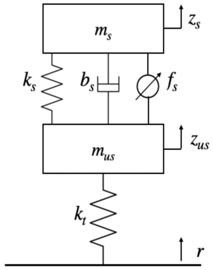
Figure 1.
Active suspension System.
The dynamic force equations of the system are the following:
with being the constant of the spring between the two masses and being the damping coefficient. represents the tire elastic constant and represents the road disturbances. The force is generated by an electro-hydraulic actuator with a servo spool valve. A schematic of the electro-hydraulic actuator is shown in Figure 2. By means of this actuator, the force is generated by the pressure supplied to the system and the area of the moving piston A. Therefore, the force can be expressed using the following equation.
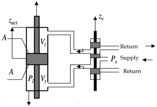
Figure 2.
Electro-Hydraulic Actuator.
The pressure dynamics are modeled using the following differential Equation (4).
with , where is the total actuator volume, Q the load flow, the effective bulk modulus, the piston leakage coefficient, the discharge coefficient, w the spool valve area gradient, the hydraulic fluid density and the pressure supply. The displacement of the spool valve is proportional to the control action which is a voltage signal. The valve displacement is expressed by the following equation.
where represents the valve gain and is a scaling factor.
3. LPV-SS Representation of the Quarter-Car Active Suspension Model
To comply with the MPC strategy, Equations (1) through (5) will be used to build a linear parameter varying state–space (LPV-SS) model with a scheduling parameter of the form:
with the discrete LPV-SS obtained by a Zero-Order Hold (ZOH) represented as:
where . With being the state matrix and the input matrix, represents the input disturbance matrix while is the control input. Therefore, the space-state matrices can be defined as the following:
With , , and . The inclusion of the scheduling variable allows the system to be expressed as an LPV-SS representation which allows the MPC law to be computed in a compact matrix form.
4. LPV-MPC Controller
To develop a MPC scheme for LPV models, the future states need to be formulated so a trajectory can be formed along the prediction horizon. The i-steps-ahead prediction can be structured as the following:
Prediction of the future states needs to be performed for the future time steps, thus using (11) the following matrix equation can be deduced.
where:
with , , and where is the number of states and the number of inputs. With the state prediction equation, we can construct a cost function to minimize the deviation from the equilibrium states and the energy used by the inputs, so that the cost function is defined as:
where and are weight matrix of appropriate dimensions. To find the optimal control trajectory , (17) needs to be minimized subject to the constraints in the inputs (18) and the states (19).
with both & and both & . However, to properly solve the MPC problem, the future values of , which are unknown, must be estimated. To obtain the values we must estimate them using an RLS approach to obtain an approximate value of the scheduling parameter based on its previous behavior and the system response.
5. Scheduling Parameter Prediction Using RLS
To obtain an estimation of the future scheduling parameter, an RLS approach is used as presented by Sename, Morato & Normey-Rico in [26]. The scheduling parameter is assumed to be measurable at instant k and all previous values can be stored; however, the future parameters will be estimated based on the previous measurements of the scheduling parameters as well as the previous inputs and outputs to consider the behavior of the system.
The behavior of the scheduling parameter of a LPV system can be approximated by a linear ARX model, which is a function of the previous scheduling parameter values, the previous inputs and the previous outputs. This ARX model can be represented as:
Afterwards, (20) can be expressed in a compact form and be dependent only on known values to be suitable for MPC design. To find a solution to the RLS, parameters to need to be calculated. These parameters will be grouped into the following vector:
resulting in:
with:
with (22) and (23) a direct solution can be built and used to find in an online RLS algorithm as presented in [30]:
with being a forgetting factor that gives exponentially less weight to older error samples of the RLS algorithm and being a vector defined as:
and is a scalar defined by:
Therefore, the RLS algorithm for estimating the future scheduling parameters is shown as Algorithm 1:
After solving the RLS algorithm for the future scheduling parameters, they will be considered to be known and exact to build a vector which contains all of them; therefore, (12) is no longer an equation with unknown variables and can be solved through LMI optimization.
| Algorithm 1 |
Offline Step 1—Initialize and Online Step 2—Obtain , and Step 3—Construct vector Step 4—Calculate scalar c Step 5—Obtain vector Step 6—Obtain Step 7—Obtain Step 8—Obtain Step 9—Set , If go to Step 10, else, go back to step 3 Step 10—Construct |
6. Quadratic Stability in MPC-LPV Approach
To ensure quadratic stability in the MPC-LPV approach, system (7) can be considered to be a parametric uncertain system. In parametric uncertain systems, the scheduling variable is limited to vary in a range . To ensure stability in parametric uncertain systems, the following condition needs to be met as presented in [31].
which is the Riccati Equation for parametric uncertain systems where is a positive definite matrix of appropriate dimensions and a static feedback gain matrix. Then, (28) can be pre- and post-multiplied by a matrix and to obtain:
To cope with the MPC paradigm, the Schur complement is applied to (29) to obtain the following LMI:
for every possible value of at time instant k which leads to an infinite number of LMI. However, as system (7) is considered to be a parametric uncertain system, (30) can be evaluated on the vertex of matrix to consider the worst-case scenarios. Therefore, (30) can be written as:
The previous condition must be met and , where l is the number of scheduling variables , is a positive definite stability matrix to be determined, and , where is the static feedback gain matrix. With these adjustments, the number of LMI to be solved is now finite and equal to . Since there is the consideration of a static feedback gain, the control law is determined as , but to comply with the MPC paradigm, the previous expression can be considered to be an inequality as . This leads to a conservative MPC performance due to the limitations of the input variable. However, this problem will be addressed in Section 7 with the inclusion of terminal sets. Therefore, using (17)–(19) and (31) the optimization problem needs to find the optimal control sequence at each time step k is the following:
7. MPC-LQR for LPV Models
7.1. Attraction Sets and Terminal Set
The inclusion of LMIs to ensure robust stability to the MPC paradigm often leads to a conservative performance of the control of the system. Therefore, to steer the system into a desired equilibrium state in the presence of disturbance or uncertainty, a series of terminal sets can be defined. In [32] a set of shrinking ellipsoids is determined using a decay rate, which can vary the speed of the system and the stability determined by similar stability conditions to the ones shown in Section 6, to steer the states to the equilibrium point. However, the determination of the decay rate and the constructions of the ellipsoids make this algorithm too slow for real-time applications and is rather implemented as an offline algorithm. In [33] a set of ellipsoidal sets are defined to predict the behavior of the system in the presence of bounded disturbances and uncertain bounded parameter changes. In [34] a path of ellipsoids is defined to predict the possible behavior of the scheduling parameter along the prediction horizon. In all three approaches, the goal of the ellipsoidal sets is that the states reach a terminal set or a terminal point, where a state-dependent stationary gain is applied to the system instead of the MPC law.
In this work, the future scheduling parameter is not known but predicted using the RLS algorithm presented in Section 3; therefore, the ellipsoids to build do not consider a variation on the scheduling parameter but rather the prediction error generated by the RLS algorithm. To generate the optimal desired trajectory to the setpoint, a path must be defined from every possible initial state to the terminal ellipsoidal set.
To steer the system into the desired terminal set, a term is added to the cost function J presented in (17). is defined as the following:
where represents the sum of the squared errors of the prediction of the future parameter values. are the predicted states at the end of the prediction horizon, represents the desired state after steps, is the predicted effect of the disturbance on the states steps ahead and it was obtained by performing an open loop simulation of every possible disturbance from every initial set of states. Both and were computed offline and stored in a lookup table. is a weighing matrix of appropriate dimensions. Therefore, (17) is redefined as:
However, the computation of every desired trajectory for every state needs to be computed offline and stored in a lookup table before the implementation of the MPC algorithm to increase execution speed.
7.2. MPC-LQR Dual Controller
To reduce the computational load of the algorithm, when the current states reach a terminal invariant set around the equilibrium point, the MPC algorithm does not need to be computed. Instead, an LQR gain can be computed based on the value of the actual prediction parameter to cope with the small error that may be present inside the terminal invariant set. The control law is then presented as:
Where is the LQR gain dependent on the scheduling parameter and is the terminal invariant set defined around the equilibrium point of the system.
Figure 3 presents the block diagram for the proposed LPV-MPC-LQR control strategy. Additionally, the LPV-MPC-LQR algorithm is shown in the flowchart presented in Figure 4.
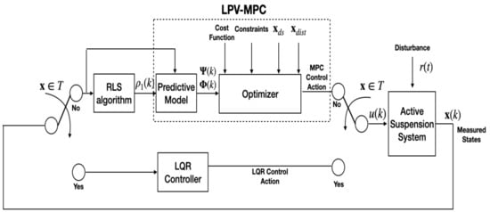
Figure 3.
Block diagram of the proposed LPV-MPC-LQR control strategy for the active suspension system.
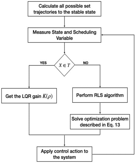
Figure 4.
Flow diagram of the LPV-MPC-LQR control strategy.
8. Results and Discussion
The following simulations are made to observe the advantages and performance of implementing the proposed LQR-MPC-LPV algorithm described in Section 7. The algorithm was tested in the active suspension system described in Section 2. Table 1 shows the specifications of the active suspension system obtained from [7].

Table 1.
Constant Values of the active suspension system.
A discretization is made to comply with the MPC paradigm using a sampling time of ms. A prediction horizon of was defined after several tests using different prediction horizons were made. Using a larger prediction horizon resulted in longer optimization time and more inexact variable scheduling predictions while it does not exhibit a significant improvement in control performance. The control objective is to steer all the states to the origin while complying with the following constraints.
The results will be divided into frequency-domain results and time-domain results.
8.1. Frequency-Domain Results
To obtain a frequency analysis in the nonlinear active suspension system, an algorithm similar to the process of defining the system response as a describing function is used. To produce these results, Algorithm 1 presented in [35] is issued. Figure 5 presents the frequency response of the active suspension deflection gain using the proposed LPV-MPC-LQR algorithm. Figure 6 presents the frequency response of the acceleration of the chassis mass using the proposed LPV-MPC-LQR algorithm; also, the frequency response plots are compared with the ones presented in [36] which use an LPV gain scheduling approach.
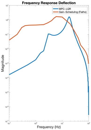
Figure 5.
Frequency response of the active suspension deflection gain.
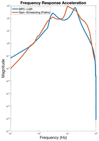
Figure 6.
Frequency response of the chassis acceleration.
The results show how the suspension deflection is attenuated at every frequency, which results in better road holding and driving conditions. Additionally, the chassis acceleration stays in values which guarantee passenger comfort. Compared to the frequency responses of the work of Fialho et al. [36] the MPC-LQR-LPV approach presents an improvement especially in terms of road holding, shown in Figure 5, without affecting the passenger comfort.
8.2. Time-Domain Results
To obtain time-domain results using the proposed LPV-MPC-LQR control algorithm, the system was simulated using two different disturbances. Figure 7, Figure 8 and Figure 9 present the suspension behavior when a bump disturbance of 5 cm is introduced. Figure 10, Figure 11 and Figure 12 show the suspension behavior when driving through a sinusoidal road. The system was simulated using Matlab®; also, the software package YALMIP [37] using QP-solver SDPT3 was used for the MPC optimization. The results presented by [7] are included to make a comparison. Additionally, the results using the MPC with a frozen scheduling parameter approach without using the RLS to show the effect of the scheduling variable prediction in control performance are included.
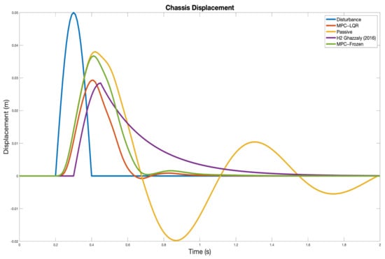
Figure 7.
Chassis displacement—Bump Disturbance (Blue—disturbance, Red—MPC-LQR, Yellow—Passive, Purple—H2, Green—MPC-Frozen).
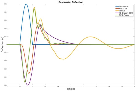
Figure 8.
Suspension Deflection—Bump Disturbance (Blue—disturbance, Red—MPC-LQR, Yellow—Passive, Purple—H2, Green—MPC-Frozen).
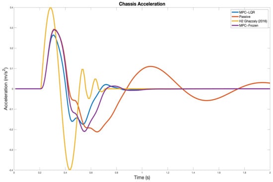
Figure 9.
Chassis Acceleration—Bump disturbance (Blue—MPC-LQR, Red—Passive, Yellow—H2, Purple—MPC-Frozen).
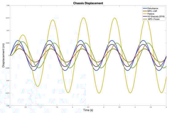
Figure 10.
Chassis displacement—Sinusoidal Disturbance (Blue—disturbance, Red—MPC-LQR, Yellow—Passive, Purple—H2, Green—MPC-Frozen).
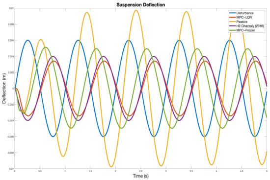
Figure 11.
Suspension Deflection—Sinusoidal Disturbance (Blue—disturbance, Red—MPC-LQR, Yellow—Passive, Purple—H2, Green—MPC-Frozen).
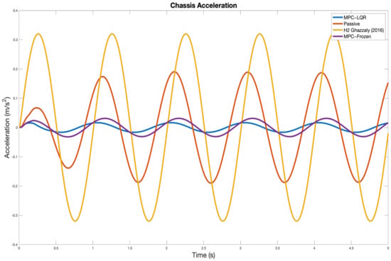
Figure 12.
Chassis Acceleration—Sinusoidal disturbance (Blue—MPC-LQR, Red—Passive, Yellow—H2, Purple—MPC-Frozen).
The results of both displacement and deflection show a better performance, which results in better road holding while maintaining passenger comfort. Additionally, the comfort exhibits improvement in terms of chassis acceleration as shown in Figure 9. Additionally, to express the results numerically, both the RMS value and the maximum value of the displacement of the chassis, the suspension deflection and the acceleration of the chassis are presented in Table 2 and Table 3 respectively.
Table 2.
RMS Values performance.
Table 3.
Max Values performance.
Similar to the bump disturbance case, the proposed LPV-MPC-LQR control strategy exhibits better performance in both displacement and deflection, which results in better road holding. In terms of comfort, the acceleration of the chassis presented in Figure 12 shows a major improvement. Table 4 presents the peak values for the displacement of the chassis, the suspension deflection, and the acceleration of the chassis.
Table 4.
Peak Values performance.
As shown in the previous figures, the proposed LPV-MPC-LQR control algorithm presents a better performance when compared with the H2 control strategy in both disturbance cases (bump disturbance and sinusoidal road disturbance). The RLS prediction of the future scheduling parameters have improved the control performance as well. Additionally, the proposed algorithm shows an appropriate optimization time with a worst optimization time of 930 ms and an average optimization time of 93 ms.
9. Conclusions
In this paper, a novel LPV-MPC-LQR control algorithm ensuring quadratic stability and with the inclusion of attraction sets was presented. This method runs an RLS algorithm to obtain the prediction of the future scheduling parameter values, which simplifies the prediction of the future states while ensuring quadratic stability. This application can cope with nonlinear systems that can be embedded into LPV representation and therefore reduce the complexity of the algorithm and allow fast execution times. This control strategy was designed and tested on a nonlinear active suspension system. The results show improvements to the performance of the active suspension in terms of road holding and passenger comfort. Future research works should deal with recursive feasibility analysis based on stability conditions, and robustness analysis. Optimization of the LPV-MPC-LQR algorithm to achieve faster execution times using techniques of the embedded systems will also be considered in future works as well.
Author Contributions
All Authors D.R.-G., A.F.-C., F.B.-C., D.S. and C.S. have contributed as follows: Conceptualization, D.R.-G., A.F.-C., F.B.-C., D.S. and C.S.; Methodology, D.R.-G., A.F.-C., F.B.-C., D.S. and C.S.; Software, D.R.-G., D.S. and C.S.; Validation, D.R.-G., A.F.-C., F.B.-C., D.S. and C.S.; Formal analysis, D.R.-G., A.F.-C., F.B.-C., D.S. and C.S.; Investigation, D.R.-G., A.F.-C., F.B.-C., D.S. and C.S.; Writing—original draft preparation, D.R.-G. and A.F.-C.; Writing—review and editing, D.R.-G., A.F.-C., F.B.-C., D.S. and C.S.; supervision, A.F.-C. and F.B.-C.; project administration A.F.-C. All authors have read and agreed to the published version of the manuscript.
Funding
This research received no external funding.
Institutional Review Board Statement
Not applicable.
Informed Consent Statement
Not Applicable.
Data Availability Statement
No new data were created or analyzed in this study. Data sharing is not applicable to this article.
Acknowledgments
The authors would like to thank Consejo Nacional de Ciencia y Tecnología (CONACyT) and Tecnológico de Monterrey for the financial support to conduct the present research. Additionally, thanks go to the Sensors and Devices Research Group and the Robotics Research Group from the School of Engineering and Sciences of Tecnológico de Monterrey for the support given to develop this work.
Conflicts of Interest
The authors declare no conflict of interest.
References
- Mouleeswaran, S. Design and development of PID controller-based active suspension system for automobiles. In PID Controller Design Approaches-Theory, Tuning and Application to Frontier Areas; Vagia, M., Ed.; Intech: Rijeka, Croatia, 2012; pp. 71–98. [Google Scholar]
- Ahmed, A.E.N.S.; Ali, A.S.; Ghazaly, N.M.; Abd el-Jaber, G.T. PID controller of active suspension system for a quarter car model. Int. J. Adv. Eng. Technol. 2015, 8, 899. [Google Scholar]
- Bello, M.M.; Shafie, A.A.; Khan, M.R. Electro-hydraulic pid force control for nonlinear vehicle suspension system. Int. J. Eng. Res. Technol. 2015, 4, 517–524. [Google Scholar]
- Phu, D.X.; An, J.-H.; Choi, S.-B. A Novel Adaptive PID Controller with Application to Vibration Control of a Semi-Active Vehicle Seat Suspension. Appl. Sci. 2017, 7, 1055. [Google Scholar] [CrossRef]
- Yu, S.; Wang, F.; Wang, J.; Chen, H. Full-car active suspension based on H2/generalised H2 output feedback control. Int. J. Veh. Des. 2015, 68, 37–54. [Google Scholar] [CrossRef]
- Afshar, K.K.; Javadi, A.; Jahed-Motlagh, M.R. Robust H∞ control of an active suspension system with actuator time delay by predictor feedback. IET Control. Theory Appl. 2018, 12, 1012–1023. [Google Scholar] [CrossRef]
- Ghazaly, N.M.; Ahmed, A.E.N.S.; Ali, A.S.; Abd, E.-J.G.T. H.∞ Control of active suspension System for a Quarter Car Model. Int. J. Veh. Struct. Syst. (IJVSS) 2016, 8, 35–40. [Google Scholar] [CrossRef]
- Kaleemullah, M.; Faris, W.F.; Hasbullah, F. Control of active suspension system using robust H∞ control with genetic algorithm. Int. J. Adv. Sci. Technol. 2019, 28, 763–782. [Google Scholar]
- Jin, X.; Wang, J.; Sun, S.; Li, S.; Yang, J.; Yan, Z. Design of Constrained Robust Controller for active suspension of In-Wheel-Drive Electric Vehicles. Mathematics 2021, 9, 249. [Google Scholar] [CrossRef]
- Wen, S.; Chen, M.Z.; Zeng, Z.; Yu, X.; Huang, T. Fuzzy control for uncertain vehicle active suspension systems via dynamic sliding-mode approach. IEEE Trans. Syst. Man Cybern. Syst. 2016, 47, 24–32. [Google Scholar] [CrossRef]
- Mustafa, G.I.; Wang, H.; Tian, Y. Model-free adaptive fuzzy logic control for a half-car active suspension system. Stud. Inform. Control 2019, 28, 13–24. [Google Scholar] [CrossRef]
- Palanisamy, S.; Karuppan, S. Fuzzy control of active suspension system. J. Vibroeng. 2016, 18, 3197–3204. [Google Scholar] [CrossRef] [Green Version]
- Alfadhli, A.; Darling, J.; Hillis, A.J. The Control of an Active Seat Suspension Using an Optimised Fuzzy Logic Controller, Based on Preview Information from a Full Vehicle Model. Vibration 2018, 1, 20–40. [Google Scholar] [CrossRef] [Green Version]
- Rath, J.J.; Defoort, M.; Karimi, H.R.; Veluvolu, K.C. Output feedback active suspension control with higher order terminal sliding mode. IEEE Trans. Ind. Electron. 2016, 64, 1392–1403. [Google Scholar] [CrossRef]
- Chokor, A.; Talj, R.; Charara, A.; Shraim, H.; Francis, C. active suspension control to improve passengers comfort and vehicle’s stability. In Proceedings of the IEEE 19th International Conference on Intelligent Transportation Systems (ITSC), Rio de Janeiro, Brazil, 1–4 November 2016; pp. 296–301. [Google Scholar]
- Taghavifar, H.; Mardani, A.; Hu, C.; Qin, Y. Adaptive robust nonlinear active suspension control using an observer-based modified sliding mode interval type-2 fuzzy neural network. IEEE Trans. Intell. Veh. 2019, 5, 53–62. [Google Scholar] [CrossRef]
- Aljarbouh, A.; Fayaz, M. Hybrid Modelling and Sliding Mode Control of Semi-active suspension Systems for Both Ride Comfort and Road-Holding. Symmetry 2020, 12, 1286. [Google Scholar] [CrossRef]
- Piñón, A.; Favela-Contreras, A.; Félix-Herrán, L.C.; Beltran-Carbajal, F.; Lozoya, C. An ARX Model-Based Predictive Control of a Semi-Active Vehicle Suspension to Improve Passenger Comfort and Road-Holding. Actuators 2021, 10, 47. [Google Scholar] [CrossRef]
- Yao, J.; Wang, M.; Li, Z.; Jia, Y. Research on model predictive control for automobile active tilt based on active suspension. Energies 2021, 14, 671. [Google Scholar] [CrossRef]
- Theunissen, J.; Sorniotti, A.; Gruber, P.; Fallah, S.; Ricco, M.; Kvasnica, M.; Dhaens, M. Regionless explicit model predictive control of active suspension systems with preview. IEEE Trans. Ind. Electron. 2019, 67, 4877–4888. [Google Scholar] [CrossRef]
- Enders, E.; Burkhard, G.; Munzinger, N. Analysis of the Influence of Suspension Actuator Limitations on Ride Comfort in Passenger Cars Using model predictive control. Actuators 2020, 9, 77. [Google Scholar] [CrossRef]
- Narayan, J.; Gorji, S.A.; Ektesabi, M.M. Power reduction for an active suspension system in a quarter car model using MPC. In Proceedings of the IEEE International Conference on Energy Internet (ICEI), Sydney, Australia, 24–28 August 2020; pp. 140–146. [Google Scholar]
- Bououden, S.; Chadli, M.; Karimi, H.R. A robust predictive control design for nonlinear active suspension systems. Asian J. Control 2016, 18, 122–132. [Google Scholar] [CrossRef]
- Wang, D.; Zhao, D.; Gong, M.; Yang, B. Research on robust model predictive control for electro-hydraulic servo active suspension systems. IEEE Access 2017, 6, 3231–3240. [Google Scholar] [CrossRef]
- Morato, M.M.; Sename, O.; Dugard, L. LPV-MPC fault tolerant control of automotive suspension dampers. IFAC-PapersOnLine 2018, 51, 31–36. [Google Scholar] [CrossRef]
- Morato, M.M.; Normey-Rico, J.E.; Sename, O. Novel qLPV MPC design with least-squares scheduling prediction. IFAC-PapersOnLine 2019, 52, 158–163. [Google Scholar] [CrossRef]
- Morato, M.M.; Normey-Rico, J.E.; Sename, O. Sub-optimal recursively feasible Linear Parameter-Varying predictive algorithm for semi-active suspension control. IET Control Theory Appl. 2020, 14, 2764–2775. [Google Scholar] [CrossRef]
- Boyd, S.; Balakrishnan, V.; Feron, E.; ElGhaoui, L. Control system analysis and synthesis via linear matrix inequalities. In Proceedings of the American Control Conference, San Francisco, CA, USA, 2–4 June 1993; pp. 2147–2154. [Google Scholar]
- Ferramosca, A.; Limón, D.; González, A.H.; Odloak, D.; Camacho, E.F. MPC for tracking target sets. In Proceedings of the 48h IEEE Conference on Decision and Control (CDC) Held Jointly with 2009 28th Chinese Control Conference, Shanghai, China, 15–18 December 2009; pp. 8020–8025. [Google Scholar]
- Franklin, G.F.; Powell, J.D.; Workman, M.L. Digital Control of Dynamic Systems; Addison-Wesley: Reading, MA, USA, 1988; Volume 3. [Google Scholar]
- Boyd, S.; El Ghaoui, L.; Feron, E.; Balakrishnan, V. Linear Matrix Inequalities in System and Control Theory; Society for Industrial and Applied Mathematics: Philadelphia, PA, USA, 1994; Chapter 5; pp. 61–76. [Google Scholar]
- Longge, Z.; Yan, Y. Robust shrinking ellipsoid model predictive control for linear parameter varying system. PLoS ONE 2017, 12, e0178625. [Google Scholar] [CrossRef] [Green Version]
- Ping, X.B.; Wang, P.; Zhang, J.F. A Multi-step Output Feedback Robust MPC Approach for LPV Systems with Bounded Parameter Changes and Disturbance. Int. J. Control Autom. Syst. 2018, 16, 2157–2168. [Google Scholar] [CrossRef]
- Suzukia, H.; Sugie, T. MPC for LPV systems with bounded parameter variation using ellipsoidal set prediction. In Proceedings of the 2006 American Control Conference, Minneapolis, MN, USA, 14–16 June 2006; p. 6. [Google Scholar]
- Poussot-Vassal, C.; Savaresi, S.M.; Spelta, C.; Sename, O.; Dugard, L. A methodology for optimal semi-active suspension systems performance evaluation. In Proceedings of the 49th IEEE Conference on Decision and Control (CDC), Atlanta, GA, USA, 15–17 December 2017; pp. 2892–2897. [Google Scholar]
- Fialho, I.; Balas, G.J. Road adaptive active suspension design using linear parameter-varying gain-scheduling. IEEE Trans. Control. Syst. Technol. 2002, 10, 43–54. [Google Scholar] [CrossRef] [Green Version]
- Lofberg, J. Automatic robust convex programming. Optim. Methods Softw. 2012, 27, 115–129. [Google Scholar] [CrossRef] [Green Version]
Publisher’s Note: MDPI stays neutral with regard to jurisdictional claims in published maps and institutional affiliations. |
© 2021 by the authors. Licensee MDPI, Basel, Switzerland. This article is an open access article distributed under the terms and conditions of the Creative Commons Attribution (CC BY) license (https://creativecommons.org/licenses/by/4.0/).