Article

Adaptive Robust Motion Control of Quadrotor Systems Using Artificial Neural Networks and Particle Swarm Optimization

by
Hugo Yañez-Badillo
1,*,
Francisco Beltran-Carbajal
2,
Ruben Tapia-Olvera
3,
Antonio Favela-Contreras
4,
Carlos Sotelo
4 and
David Sotelo
4
1
Departamento de Investigación, Tecnológico de Estudios Superiores de Tianguistenco, Santiago Tilapa 52650, Mexico
2
Departamento de Energía, Universidad Autónoma Metropolitana, Unidad Azcapotzalco, Mexico City 02200, Mexico
3
Departamento de Energía Eléctrica, Universidad Nacional Autónoma de México, Mexico City 04510, Mexico
4
Tecnologico de Monterrey, School of Engineering and Science, Ave. Eugenio Garza Sada 2501, Monterrey 64849, Mexico
*
Author to whom correspondence should be addressed.
Mathematics 2021, 9(19), 2367; https://doi.org/10.3390/math9192367
Submission received: 3 August 2021 / Revised: 31 August 2021 / Accepted: 10 September 2021 / Published: 24 September 2021

Abstract

:
Most of the mechanical dynamic systems are subjected to parametric uncertainty, unmodeled dynamics, and undesired external vibrating disturbances while are motion controlled. In this regard, new adaptive and robust, advanced control theories have been developed to efficiently regulate the motion trajectories of these dynamic systems while dealing with several kinds of variable disturbances. In this work, a novel adaptive robust neural control design approach for efficient motion trajectory tracking control tasks for a considerably disturbed non-linear under-actuated quadrotor system is introduced. Self-adaptive disturbance signal modeling based on Taylor-series expansions to handle dynamic uncertainty is adopted. Dynamic compensators of planned motion tracking errors are then used for designing a baseline controller with adaptive capabilities provided by three layers B-spline artificial neural networks (Bs-ANN). In the presented adaptive robust control scheme, measurements of position signals are only required. Moreover, real-time accurate estimation of time-varying disturbances and time derivatives of error signals are unnecessary. Integral reconstructors of velocity error signals are properly integrated in the output error signal feedback control scheme. In addition, the appropriate combination of several mathematical tools, such as particle swarm optimization (PSO), Bézier polynomials, artificial neural networks, and Taylor-series expansions, are advantageously exploited in the proposed control design perspective. In this fashion, the present contribution introduces a new adaptive desired motion tracking control solution based on B-spline neural networks, along with dynamic tracking error compensators for quadrotor non-linear systems. Several numeric experiments were performed to assess and highlight the effectiveness of the adaptive robust motion tracking control for a quadrotor unmanned aerial vehicle while subjected to undesired vibrating disturbances. Experiments include important scenarios that commonly face the quadrotors as path and trajectory tracking, take-off and landing, variations of the quadrotor nominal mass and basic navigation. Obtained results evidence a satisfactory quadrotor motion control while acceptable attenuation levels of vibrating disturbances are exhibited.

1. Introduction

It is known that, in motion control systems, it is required that the system move to match some desired features of acceleration, velocity, position, or a combination of them. Unmanned aerial vehicles (UAVs) are dynamic systems where the controlled motion is fundamental to complete specific applications. Recently, diverse types of UAVs vehicles have been developed, with fixed-wing unmanned aerial vehicles (FW-UAVs) being the most common and most developed. These aircraft are similar to passenger aircraft, with a pair of wings to provide lift, a propellant system to provide thrust, and aerodynamic surfaces to control the motion. Their efficiency is higher compared to other UAVs, allowing it to perform long flights. Nevertheless, their indoors use is exclude since they do not have the ability to hovering and can not turn at reduced distances [1]. For their part, rotary-wing unmanned aerial vehicles (RW-UAVs) have various configurations including the conventional helicopter, the coaxial helicopter, and multi-rotors, which can sustain hover flight and take-off-landing vertically (VTOL). The FW-UAVs and RW-UAVs are the classic configurations most used in the applications assigned to unmanned aerial vehicles. Among the main ones are surveillance, monitoring, photography, inspection, and cargo transportation [2], with RW-UAVs having more civil applications than FW-UAVs [3]. On the other hand, technological advances have also allowed the development of new UAV configurations, such as bio-inspired flapping-wing unmanned aerial vehicles (Fl-UAV) [4] and lighter-than-air unmanned aerial vehicles, (LtA-UAVs) [5]. The four rotor helicopter or quadrotor is the most common rotorcraft platform in the research community due to its properties of under-actuation, low construction cost, symmetrical structure, high coupling non-linear dynamics, and capabilities of VTOL and hovering.
In the literature, several important contributions have been reported for controlling the quadrotor dynamics. Motion controllers based on theories, such as sliding modes [6], active disturbance rejection [7], backstepping [8], Lyapunov functions [9], H [10], adaptive controllers based on L 1 [11,12], fuzzy logic [13], neural networks [14], model predictive control [15], or combination of them. Since, to some, drawbacks are inherent to each control strategy, such as high-frequency control actions, unmeasurable system information required, high dependency of mathematical models, high-gain feedback, and high sensibility against exogenous disturbances, some researchers have been properly exploited the properties of adaptive and robust control for designing advanced control methodologies.
In contrast with conventional control, intelligent control techniques are able to efficiently deal with incomplete information of many dynamic systems and its environment within a wide range of operational conditions. Then, adaptive control strategies represent a potential alternative for improving the performance of robust motion control schemes. In the literature, adaptive control stands for a class of control techniques used for compensating parameter changes, disturbances, and unknown changes in the system, by adaptations based on observations [16]. Relevant and recently research have been inspired by the qualities of adaptive and robust control schemes for quadrotor motion control. Authors in [17] introduce a model reference adaptive control scheme for a four-rotor helicopter in order to increase robustness against parametric uncertainty. A baseline controller is proposed for trajectory tracking task which is further improved by including adaptive capabilities. Similarly, switched adaptive controller are properly introduced in [18,19]. Here, controllers are suitably designed for controlling a quadrotor in the presence of unknown external disturbances and variations in the mass and inertia of the quadrotor due to unknown payload. Strict simulation scenarios are brought out to validate their proposal.
On the other hand, another adaptive control scheme is presented by authors in [20], where the quadrotor attitude is stabilized by an adaptive multi-variable finite-time algorithm. The controller design is carried out by using an improved super-twisting technique. Control methodologies designed based on the central ideas of adaptive sliding mode control are presented in [21,22]. In [21], a disturbance observer (DO) is integrated in control design to compensate external disturbances. The tune of the gain of sliding surface is accomplished via neural networks. In contrast, authors in [22] implement an adaptive scheme by proposing a super twisting controller along with Lyapunov-based function methodology and discontinuous projection operators. The research in [23] presents a fuzzy adaptive linear active disturbance rejection controller. The fuzzy framework is setup successfully to compute the observer bandwidth, controller bandwidth, as well as the control compensation factor.
Considering the aforementioned information, in this paper, authors introduce a novel and efficient adaptive robust motion tracking control for quadrotor non-linear systems. The main differences with others proposals reported in the literature are enlisted below:
  • Only position measurements are required for feedback control;
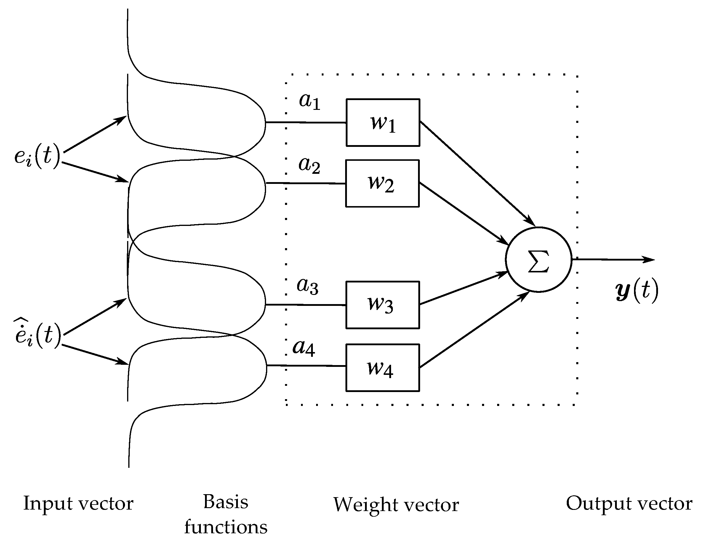
  • High-gain feedback is reduced by using B-spline artificial neural networks;
  • Reduced amount of control parameters needs to be tuned;
  • The use of disturbance observers is unnecessary;
  • The use of the tracking error derivatives is avoided in the controller design;
  • Offline training of B-spline artificial neural networks is performed by particle swarm optimization;
  • Low dependency of the quadrotor non-linear mathematical model;
  • Robustness against a class of external disturbances, including undesirable vibrating forces and torques.
The content of this paper is summarized as follows: the quadrotor non-linear and high coupling mathematical model is presented in Section 2. In Section 3, the design procedure of the novel robust and adaptive controller is introduced. Subsequently, some simulation experiments are presented in Section 4 in order to highlight the performance of the introduced methodology. Finally, some conclusions, remarks, and future work are mentioned in conclusions section.

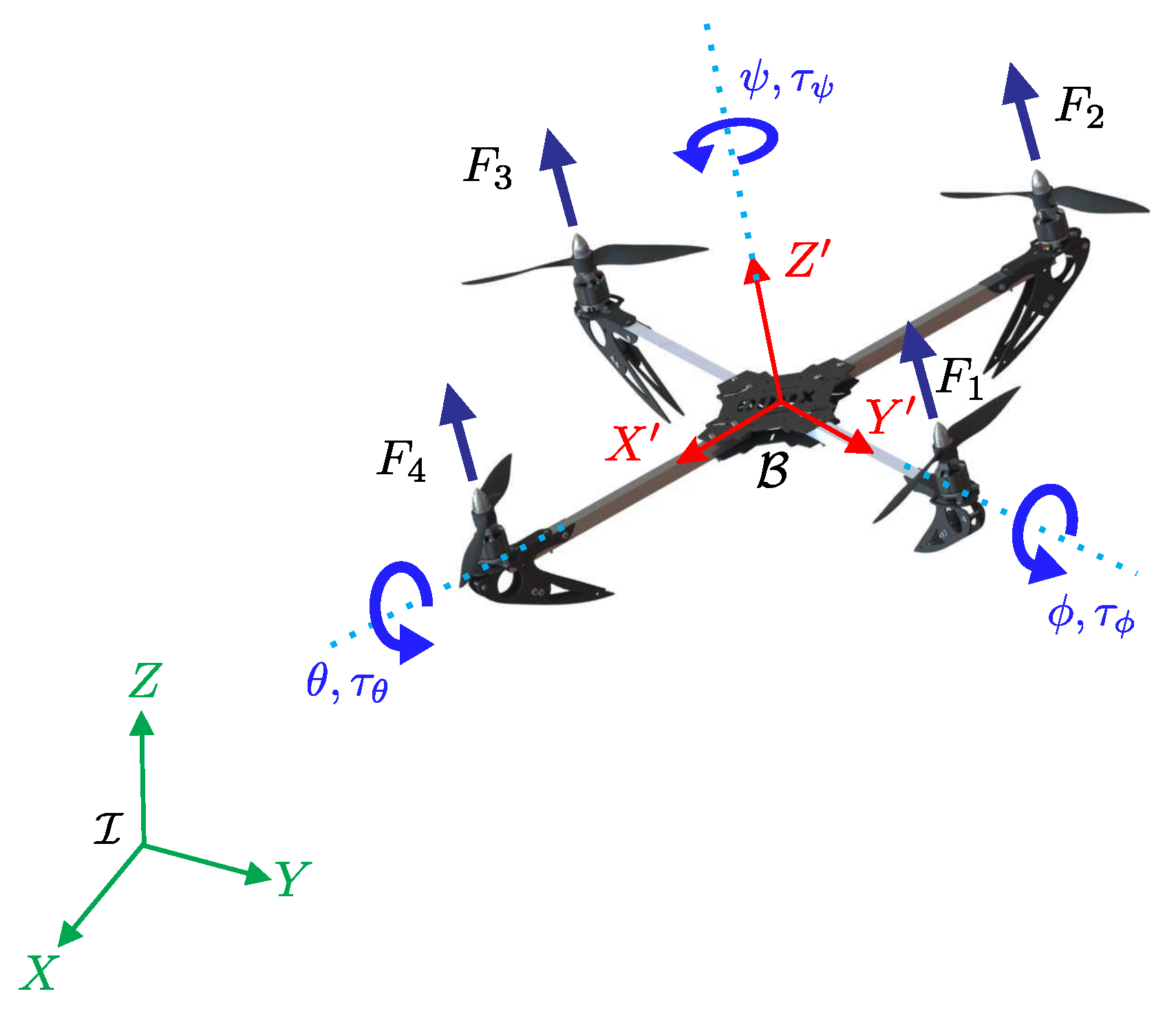
2. Mathematical Quadrotor Model

A quadrotor is an aerial under-actuated mechanical system with four independent variable speed rotors. It has six degrees of freedom which are controlled by four control inputs: a main thrust force (u), and three torques (rolling τ ϕ , pitching τ θ , and yawing τ ψ ). Lateral, longitudinal, and vertical motion are achieved by a suitable combination of the control inputs. The main force, produced by the total sum of the thrust provided by each individual rotor, allows the quadrotor to take-off and land, as well as hover. Meanwhile, control torques are generated when there exists a difference of the produced forces by two pair of rotors: first pair rotating clockwise is formed by rotors 1 and 3, and the second by 2 and 4 rotors spinning in the opposite direction. Different from conventional helicopters it is not required a mechanical pitch system for the rotor blades.
The Euler–Lagrange and Newton–Euler formalisms are usually used to obtain the quadrotor dynamics described by a set of highly coupled non-linear differential equations. The quadrotor pose is determined by considering a body-fixed frame with X , Y , and Z axes coincident with the centre of mass, and a global inertial coordinate system, or earth-fixed frame, with X, Y, and Z axes, as shown in Figure 1. By nature the quadrotor is an unstable system, and during outdoor and indoor flying, quadrotors might be subjected to undesirable vibrating disturbances. Thus, it should be designed efficient force and torque controllers to perform a proper motion tracking in the three-dimensional space.
The control inputs are related with each individual rotor by the following expressions
u = i = 1 4 F i τ ψ = i = 1 4 τ M i τ θ = F 3 F 1 l τ ϕ = F 2 F 4 l
here l stands for the distance measured from a rotor axis to the quadrotor centre of mass, and τ M i is the couple developed by motor M i . F i and τ M i are functions of the rotor angular velocities. From Equation (1) it is appreciated that the quadrotor motion is possible by suitably combining the control inputs.
In this work, the non-linear dynamic model of the quadrotor is derived by means of the Euler–Lagrange formalism. In order to describe the system, let us consider the following vector of generalized coordinates
q = x y z ϕ θ ψ R 6
the centre of mass position is represented by the variables x, y, and z, and the quadrotor attitude is described by the set of Euler roll ϕ , pitch θ , and yaw ψ angles.
The Lagrangian is defined by the difference of the kinetic and potential energy, so we get
L = 1 2 λ ˙ M λ ˙ + 1 2 η ˙ J η ˙ λ M G
M indicates a diagonal mass matrix, J is the inertia tensor, and G = 0 0 g denotes gravity terms. Henceforth, consider λ = x y z and η = ϕ θ ψ as the position and attitude vectors, both expressed in the earth-fixed reference frame.
For controller design, the non-linear quadrotor dynamics can be written as
m x ¨ = u sin θ + ξ x m y ¨ = u cos θ sin ϕ + ξ y m z ¨ = u cos θ cos ϕ m g + ξ z
unknown time-varying disturbances are represented by ξ x , ξ y , and ξ z . On the other hand, disturbed rotational dynamics are given by
J η ¨ = τ η C ( η ˙ , η ) η ˙ + ξ η
with
J = I x s θ 0 I x ( I y I z ) c θ c ϕ s ϕ I y c ϕ 2 + I z s ϕ 2 0 I z c θ 2 c ϕ 2 + I y c θ 2 s ϕ 2 + I x s θ 2 ( I y I z ) c θ c ϕ s ϕ I x s θ C ( η ˙ , η ) = c 11 c 12 c 13 c 21 c 22 c 23 c 31 c 32 c 33
and
c 11 = ( I z I y ) ψ ˙ s ϕ c ϕ c θ 2 c 12 = I x ψ ˙ c θ + I y ( θ ˙ s ϕ c ϕ + ψ ˙ c θ s ϕ 2 ψ ˙ c θ c ϕ 2 ) I z ( ψ ˙ c θ s ϕ 2 ψ ˙ c θ c ϕ 2 + θ ˙ s ϕ c ϕ ) c 13 = 0 c 21 = I x ψ ˙ s θ c θ + I y ψ ˙ s θ c θ s ϕ 2 + I z ψ ˙ s θ c θ c ϕ 2 c 22 = ( I z I y ) ϕ ˙ s ϕ c ϕ c 23 = I x ψ ˙ c θ + I y ( θ ˙ s ϕ c ϕ + ψ ˙ c θ c ϕ 2 ψ ˙ c θ s ϕ 2 ) + I z ( ψ ˙ c θ s ϕ 2 ψ ˙ c θ c ϕ 2 + θ ˙ s ϕ c ϕ ) c 31 = θ ˙ I x s θ c θ + I y ( θ ˙ s θ c θ s ϕ 2 + ϕ ˙ s ϕ c ϕ c θ 2 ) I z ( θ ˙ s θ c θ c ϕ 2 + ϕ ˙ s ϕ c ϕ c θ 2 ) c 32 = I x ψ ˙ s θ c θ I y ( θ ˙ s θ s ϕ c ϕ + ϕ ˙ c θ s ϕ 2 ϕ ˙ c θ c ϕ 2 + ψ ˙ s θ c θ s ϕ 2 ) + I z ( ϕ ˙ c θ s ϕ 2 ϕ ˙ c θ c ϕ 2 ψ ˙ s θ c θ c ϕ 2 + θ ˙ s θ s ϕ c ϕ ) c 33 = I x θ ˙ c θ + ( I y I z ) ( ψ ˙ c θ 2 s ϕ c ϕ )
For purposes of simplicity of the model representation, the shorthand notation for trigonometric functions is adopted [25], where s b = sin b and c a = cos a . On the other hand, the control and disturbance torque vectors are denoted by τ η = [ τ ϕ τ θ τ ψ ] T and ξ η = [ ξ ϕ ξ θ ξ ψ ] T , respectively.
Since the quadrotor is an under-actuated non-linear system, two synthetic controllers are designed for tracking tasks of some desired reference position trajectory on the plane. For control design purposes, it is considered the output feedback errors given as follows
e μ = μ μ
for μ = x , y , z , ϕ , θ , ψ . The superscript stands for the desired reference trajectory. Moreover, in order to perform a proper motion control in X and Y directions, the desired pitch θ and roll ϕ references are computed from Equation (4) as follows
θ = sin 1 1 u m v x ϕ = sin 1 1 u cos θ m v y
To solve adequately the under-actuation problem, the angular dynamics needs to be faster than translational dynamics. In this way, the proposed motion controllers should be capable to lead the quadrotor to stable scenarios while performing a proper tracking of the planned references.

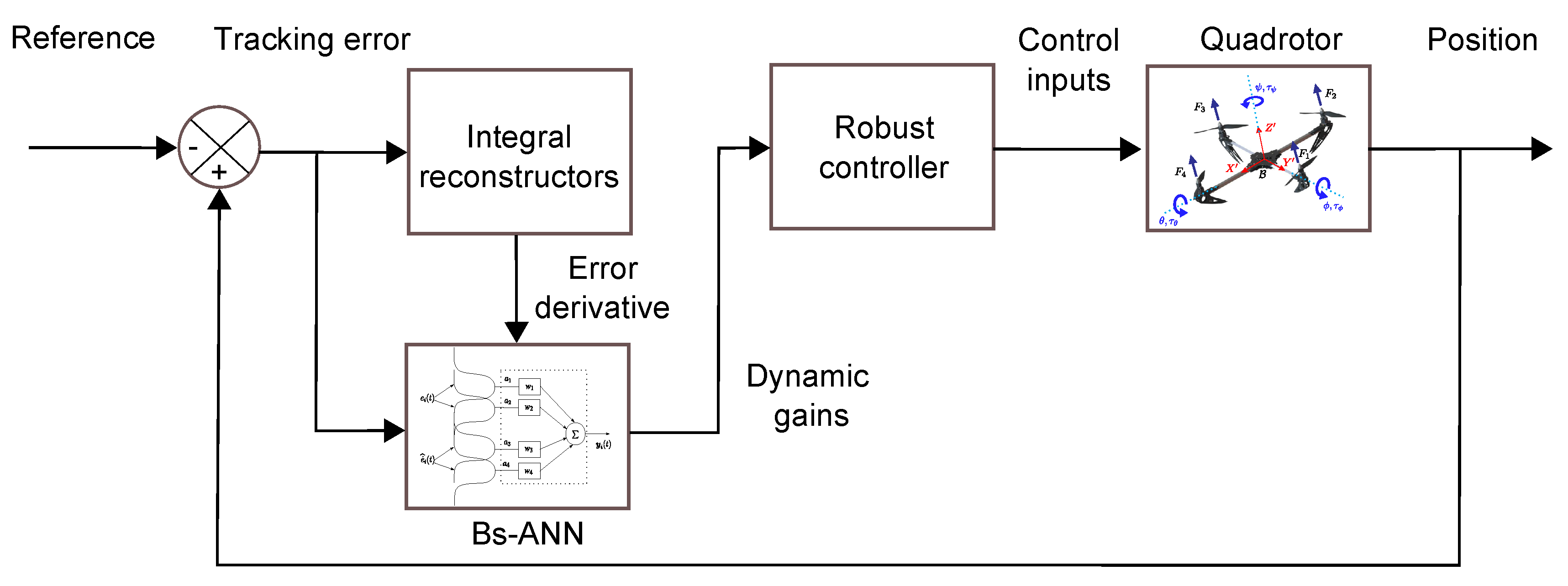
3. Syntheses of an Adaptive Robust Motion Controller

The syntheses of a novel adaptive robust motion controller is introduced in this section by using the robust control scheme introduced by the authors in [24]. In this proposal, it is improved the performance of the control scheme by reducing the high-gain effects and easing the tuning of the control parameters computed online by using the Bs-ANN.

3.1. Dynamic Compensators for Robust Control Design

In order to realize the stable control design, the quadrotor disturbed tracking error dynamics from Equations (4) and (5) are simplified as follows
e ¨ μ = v μ + ξ μ ( t )
Moreover, ξ μ ( t ) are assumed to be bounded time-varying disturbance signals locally approximated into a self-adaptive small interval of time around a given time instant t 0 > 0 , say [ t 0 , t 0 + ε ] , by r-th order Taylor polynomials as
ξ μ ( t ) n = 0 r ξ μ ( n ) ( t 0 ) n ! ( t t 0 ) n = n = 0 r σ n , μ ( t t 0 ) n
where the superscript ( n ) stands for n-th order time derivative. Furthermore, to avoid velocity measurements, from Equation (9) structural estimates—known as integral reconstructors as well [26]—for time derivatives of velocity tracking errors are computed by
e ˙ ^ μ = t 0 t v μ d t
Here, initial conditions of the non-linear dynamic system, as well as the polynomial disturbance signal parameters are assumed to be completely unknown. Then, the polynomial relationship between integral reconstructors e ˙ ^ μ and actual velocity tracking error signals e ˙ μ is given by
e ˙ μ = e ˙ ^ μ + n = 0 r + 1 α n , μ ( t t 0 ) n
where parameters α n , μ are assumed to be unknown as well.
In this fashion, the following family of controllers based on dynamic compensators to actively compensate polynomial disturbances can be synthesized as follows
v μ = β r + 3 , μ e ˙ ^ μ β r + 2 , μ e μ δ r + 1 , μ
with
δ ˙ 0 = β 0 , μ e μ δ ˙ 1 = δ 0 , μ + β 1 , μ e μ δ ˙ r = δ r 1 , μ + β r , μ e μ δ ˙ r + 1 , μ = δ r , μ + β r + 1 , μ e μ
Substitution of Equation (13) into Equation (9), closed-loop tracking error dynamics is then described by
e μ ( r + 4 ) + n = 0 r + 3 β n , μ e μ ( n ) = 0
Thus, closed-loop system stability criteria is fulfilled by selecting the control gains β k , μ for k = 0 , 1 , , r + 3 , such a way the characteristic polynomial of Equation (15) is stable (Hurwitz). By using the family of Hurwitz polynomials
P C L μ ( s ) = s + γ μ r + 4 , γ μ > 0
the control design parameters can be then computed by
β k , μ = r + 4 ! k ! r + 4 k ! γ μ r + 4 k
In the present study, three layers B-spline artificial neural networks and particle swarm optimization are properly implemented to compute adaptive control gains in order to avoid possible undesirable high-gain control effects. Furthermore, first order Taylor polynomial expansions for approximation of disturbance signals are selected. Nevertheless, higher order polynomial expansions can be also chosen for applications where a much better approximation of disturbances is demanded. In this work, it is shown that first order polynomial disturbance approximations yield an acceptable motion trajectory tracking performance under significantly perturbed operating conditions.
Thus, from Equation (10), Taylor polynomial expansions for disturbance signals are described in this work as
ξ μ ( t ) σ 1 , μ + σ 2 , μ ( t t 0 )
where coefficients σ 1 , μ and σ 2 , μ are assumed to be uncertain. Moreover, the structural estimated variables and actual velocity tracking error signals are related by
e ˙ μ = e ˙ ^ μ + α 0 , μ ( t t 0 ) + α 1 , μ ( t t 0 ) 2
where parameters α i , μ are unknown.
In this sense, we proposed the following family of auxiliary controllers for robust quadrotor motion control
v μ = β 4 , μ e ˙ ^ μ β 3 , μ e μ β 2 , μ δ 1 , μ β 1 , μ δ 2 , μ β 0 , μ δ 3 , μ
with
δ ˙ 1 , μ = e μ δ ˙ 2 μ , = δ 1 , μ δ ˙ 3 , μ = δ 2 , μ
Thence, from Equations (9) and (20) the closed-loop error dynamics is governed by
e μ ( 5 ) + β 4 , μ e μ ( 4 ) + β 3 , μ e μ ( 3 ) + β 2 , μ e ¨ + β 1 , μ e ˙ + β 0 , μ e μ = 0
The control gains β k , μ for k = 0 , 1 , , 4 should be properly selected in order to the associated characteristic polynomials
P C L μ ( s ) = s 5 + β 4 , μ s 4 + β 3 , μ s 3 + β 2 , μ s 2 + β 1 , μ s + β 0 , μ
are Hurwitz polynomials. In this fashion, reference trajectory tracking can be achieved:
lim t e μ = 0 lim t μ = μ
with μ and μ standing for the real and planned references for translational and rotational trajectories, respectively.
Notice from (5) that the rotational dynamic model can be also be expressed as follows:
η ¨ = J 1 τ η C ( η ˙ , η ) η ˙ + J 1 ξ η
which can be expressed matching the structure in (9). Therefore, from (21) it is observed that the synthetic controllers drive the system closed-loop dynamics. Finally, by analyzing the full non-linear dynamics, the control inputs nature and the robustness of the synthesized robust scheme, a suitable selection of the control inputs is given as follows
u = 1 cos ϕ cos θ m v z + m g τ ψ = I z v ψ τ θ = I y v θ τ ϕ = I x v ϕ

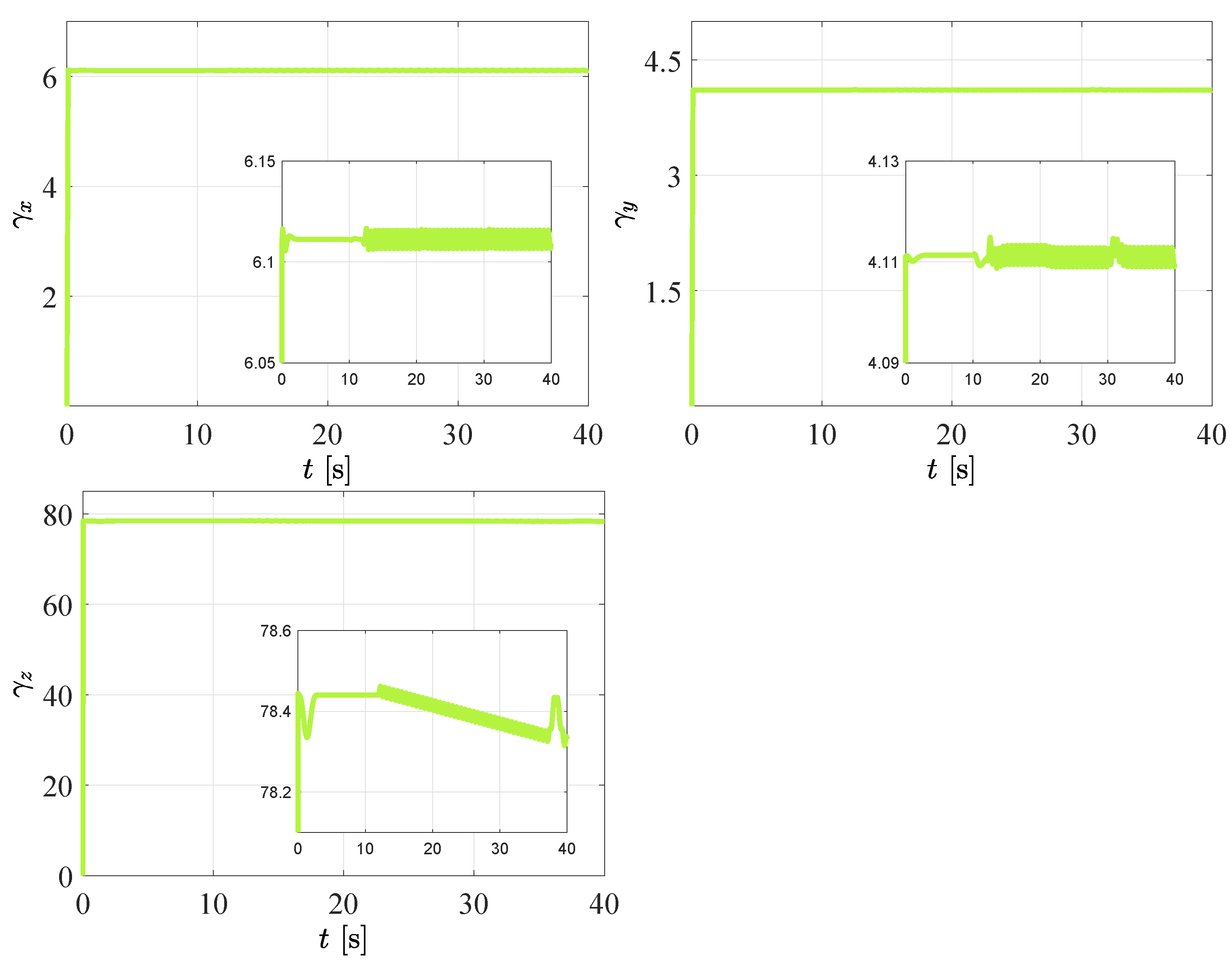
3.2. Adaptive Outline for Control Purposes

Adaptive control is a viable solution to avoid the use high-gain feedback or high frequency switching control actions for providing stability to many dynamic systems subjected to parametric uncertainty, unmodeled dynamics, and external disturbances [27]. In this work, we use a class of artificial neural networks for performing the tuning process of the control gains. The B-spline artificial neural networks are suitably integrated into adaptive motion controllers, where the tracking errors and their derivatives are used as the inputs of each network. The Bs-ANN functioning is based on the constant learning process of the physically system variables, therefore, have been successfully used to deal with system non-linear terms and uncertainty [28].
A B-spline function is a polynomial mapping defined by its extremes which uses a linear combination of the mono-variable and multi-variable basis functions. The B-spline networks, as depicted in Figure 2, are associative networks capable to adjust iteratively their synaptic weights for reproducing a specific function. The author in [29] proposes the following output:
y = a w , w = w 1 w 2 w h T , a = a 1 a 2 a h
where w q y a q are the q-th weight and the q-th basis function input, respectively; the quantity of synaptic weights is denoted by h. Each individual network output y ( t ) is used in this work for computing dynamically the control gains. In this study, we introduce different experiments where the output of the neural networks differs: in experiments 1, 2, 4, and 5, it is computed just one control parameter while in experiment 3, three control parameters are computed by the adaptive scheme.
The actual output vector value minus the desired value defines the minimization error, which is used as the key term for the learning process. In this work, the following instantaneous learning rule has been adopted [30]
w i t = w i t 1 + e i t a t 2 2 a i t
Here, represents the learning rate and e i ( t ) stands for the instantaneous output error. The adaptive process is achieved by the continuous training and the updating of the synaptic weights values considering the evolution of the inputs values. The Bs-ANN internal layer is constituted just by the basis functions, where the limits should be properly bounded by the adequate selection of the knot vector and basis function shape. In this proposal, four third order basis functions are employed for the adaptive scheme: two concerning the tracking error and two for the error derivative, as shown in Figure 2. It is important to mention that offline training of the Bs-ANN is performed for finding parameters during the adaptive scheme design process, in order to carry out the quadrotor to stable scenarios at the begging of the online training. To select properly these parameters, several quadrotor operational conditions are considered. The training data includes the transient and steady state response of the system, within the advantages of the proposed neural strategy, is that these data can come from an exact or approximate mathematical model or otherwise be measured data from the real system (inputs, outputs, control signals, etc.).
Thereafter, the control structure is summarized as follows: firstly, only the quadrotor position measurements are included as a feedback in order to determine the tracking errors. Later, integral reconstructors are suitably integrated for computation of the error derivatives which are used as inputs in the adaptive scheme for computing the control parameters and gains. Posteriorly, the virtual controllers v x and v y within the robust controller block are used for solving the under-actuation problem. Finally, the force and torque control inputs are injected to the system as variations of angular velocity of their four rotors, as portrayed in Figure 3.

4. Validation through Simulation Experiments

In this section, we investigate the applicability of the adaptive robust scheme for enhancing the tracking performance of a quadrotor non-linear system. Thus, several experiments are performed for an aerial vehicle numerically simulated. It is important to mention that the aim of the experiments is to portray some of the main contributions and advantages of implementing the proposed motion control strategy. Additionally, the experiments will demonstrate if the implementation of the proposal can be successfully extended for motion control of different types of autonomous vehicles. During the experiments, it is considered an aerial vehicle characterized by the set of parameters presented in Table 1.

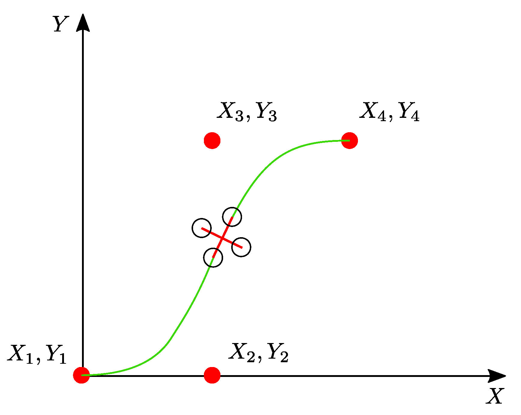
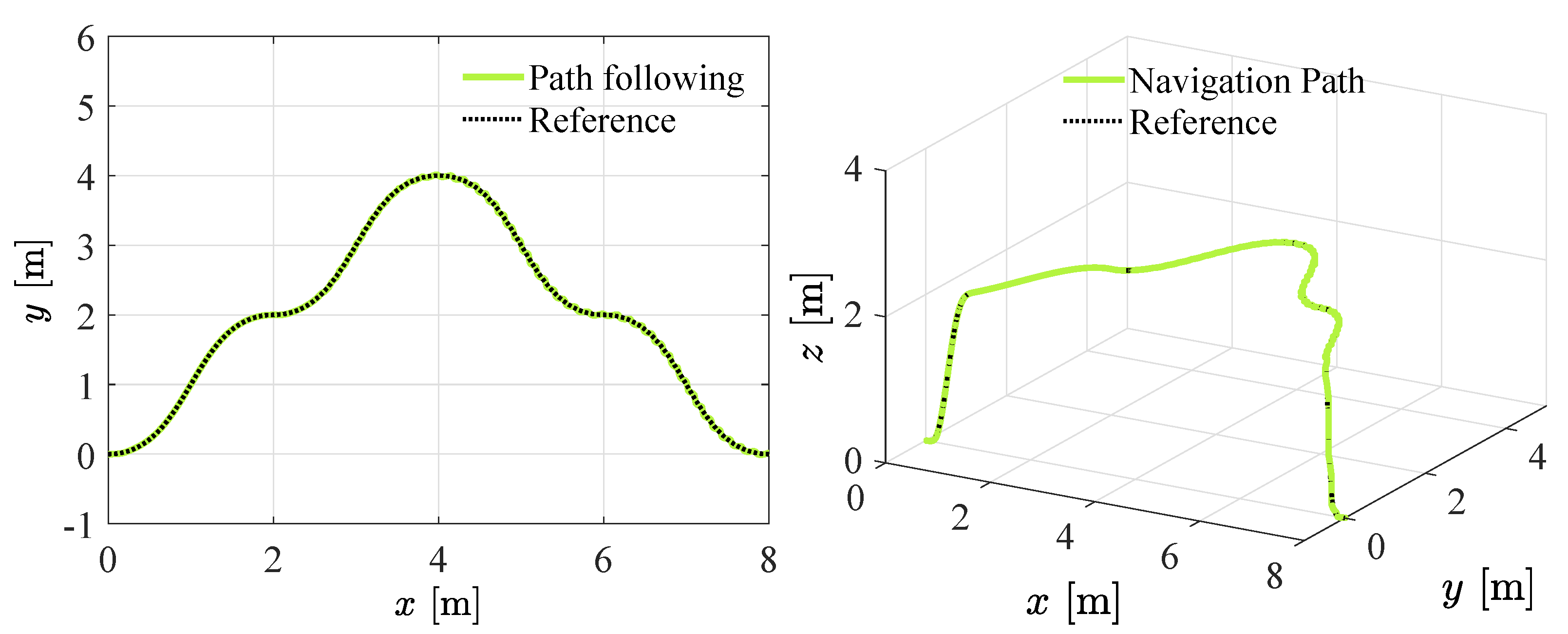
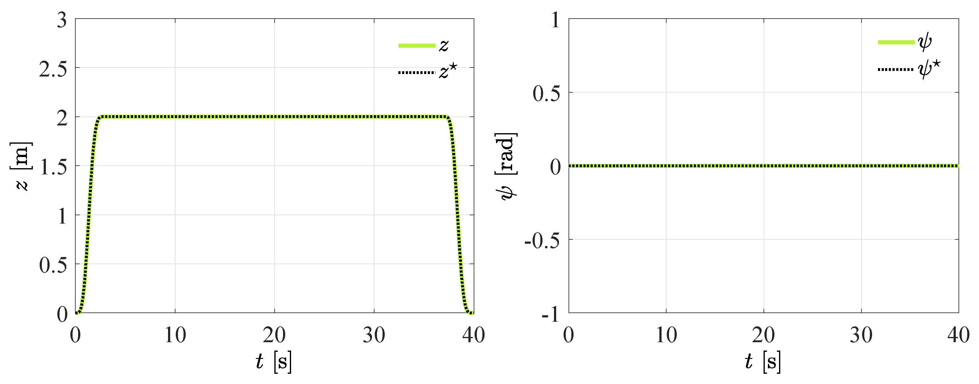
4.1. Polynomial Interpolation for Quadrotor Navigation

Bézier curves have been used widely and properly for path smoothing in robot navigation [31] and in motion control schemes for electric motors [32] and mechanical systems [33]. In the former, curves are expressed, such as parametric equations, where the time t is used to determine the values of coordinate pairs of ( x , y ) points graphed on the plane. In this work, a cubic Bézier curve is used and is defined by end points: ( X 1 , Y 1 ) and ( X 4 , Y 4 ) , and control points: ( X 2 , Y 2 ) and ( X 3 , Y 3 ) such illustrated in Figure 4. In the second case, Bézier interpolation polynomials are suitably configured as position or velocity trajectory reference profiles, in order to soft the transition between two operation points for electromechanical and mechanical systems.
It is worthwhile to note that, due to its structure and after a proper selection of endpoints and control points, Bézier curves can be successfully implemented in a quadrotor to online computing the navigation path in cluttered environments, in order to ensure adequate obstacle avoidance manoeuvres while accomplishing a specific mission. On the other hand, it should be noted that derivatives of the trajectory references are not available in advance, and, in consequence, the proposed approach in this paper can be effectively implemented for this experiment.
During the first experiment, the quadrotor is tasked to perform the following: soft take-off to a height of 3 m; navigation through specific operation points in the space; and finally, soft landing, all of them by means of Bézier curves. It is worthwhile to note that the use of these curves is a viable strategy for solving properly the navigation and obstacle avoidance problems. Thus, in order to obtain smooth transitions between initial and final vertical operation points, the following motion scheme is adopted for take-off and landing tasks:
z = Γ 0 0 t < T 1 Γ 0 + Γ m Γ 0 B z ( t , T 1 , T 2 ) T 1 t < T 2 Γ m T 2 t < T 3 Γ m + Γ 0 Γ m B z ( t , T 3 , T 4 ) T 3 t < T 4 Γ 0 t > T 4
where Γ 0 = 0 and Γ f = 2 , given in meters, stand for the desired initial and maximum vertical positions. The time values given in seconds are as follows: T 1 = 1 , T 2 = 3 , T 3 = 37 and T 4 = 40 . In addition, B z is a Bézier polynomial [32] defined as
B z ( t , T i , T f ) = k = 0 n r k t T i T f T i k
with T i and T f as the initial and final transition times. Moreover, n = 6 , and r 1 = 252 , r 2 = 1050 , r 3 = 1800 , r 4 = 1575 , r 5 = 700 , r 6 = 126 .
Subsequently, after the take-off, the rotorcraft is carry to desired positions in the horizontal plane, where the third order parametric equations used for navigation are defined as follows:
x = ( 1 T ) 3 X 1 + 3 ( 1 T ) 2 ( T X 2 ) + 3 ( 1 T ) ( T 2 X 3 ) + T 3 X 4 y = ( 1 T ) 3 Y 1 + 3 ( 1 T ) 2 ( T Y 2 ) + 3 ( 1 T ) ( T 2 Y 3 ) + T 3 Y 4
Here, the values of the endpoints and control points are selected for performing a continuous navigation according to the parameters summarized in Table 2. Observe that four Bézier curves are used to define the whole navigation path and which is segmented for purposes of mathematical description.
On the other hand, external vibrating disturbance forces have been included after 12 s for robustness assessment purposes of the introduced motion control scheme, and are given by
ξ j = A j sin ( ω j t )
with j = x , y , z , A x = A y = 1   N , A z = 2   N , and ω x = ω y = ω z = 10   rad / s .
In Figure 5, it is presented the quadrotor flight performance by implementing the proposed controller, where a proper path following is exhibited. Throughout the manuscript, the use of solid and dashed lines for representing real and desired trajectories is adopted, respectively. As observed in Figure 6, the Bézier curves are successfully implemented for navigation between operation positions, and as a consequence of the proposed controller, a proper trajectory tracking of the planned references is achieved. Moreover, according to this figure, angular tracking of the online computed references ϕ and θ is achieved in spite of there is not information about the derivatives of these references since a properly integration of integral reconstructors and neural networks within the robust motion control approach is achieved.
Furthermore, it is evident the satisfactory performance of the quadrotor tracking motion control scheme even though the quadrotor is subjected to undesired harmonic forces. Notice that regulation around ψ = 0 rad is performed in this experiment. Additionally, Figure 7 portrays the controlled vertical quadrotor dynamics, the height control, and yaw motion regulation. From this figure, the utility of the Bézier polynomial curve, where a soft take-off and landing are achieved thanks to the mathematical framework introduced by Equations (30) and (52) is appreciated. In the next section, the ground effect is included within the analysis in order to assess the control scheme robustness for controlling the quadrotor vertical motion.
For this experiment the following desired Hurwitz polynomial has been selected,
P d s = ( s + γ 2 ) 5
where, in order to ensure close-loop stability and the properly tracking of the planned trajectory, the control gains in (23) should match the following
β 4 i = 5 γ i β 3 i = 10 γ i 2 β 2 i = 10 γ i 3 β 1 i = 5 γ i 4 β 0 i = γ i 5
where γ i , for i = x , y , z , ϕ , θ , ψ , is the unique online computed control parameter. To improve and ease the parameter selection process in this experiment, each of these control parameters are suitably derived by the adaptive framework introduced in Figure 2, where the output of each individual neural network is the value for the control parameter γ i . As it is presented in Figure 8, dynamical updating, as well as a successful parameter computation of the control gains, is achieved by using the adaptive B-spline artificial neural networks.
In Figure 9, it has been included results considering both perturbed and unperturbed cases in order to contrast the compensation action of the adaptive robust control scheme. It is worthwhile to note, from Figure 9b, that it is possible to track, satisfactorily, the references, as well as being demonstrated in Figure 9a. Nevertheless, the vibrating disturbance compensation is not present in the unperturbed case. By analyzing Figure 9b, it is evident the reachability of the control commands which benefits the non-saturation of the actuators. It is also important to mention that similarly as the oscillations due to the control compensation action, in Figure 6 it is appreciated the compensation of the vibrating disturbance forces affecting translational dynamics since are related with the rotational trajectory tracking trough the under-actuation property.
According to the results, the proposed control method is robust and able to efficiently reduce induced oscillations. Additionally, it is demonstrated that Bézier polynomial interpolation can be widely and satisfactorily exploited in quadrotor motion control systems: path and trajectory tracking. The experiment presented in this section illustrates that the complex quadrotor non-linear system is motion controlled in an acceptable way. As no information is required about derivatives of the trajectory references and from the external disturbances the control process is simplified significantly.

4.2. Improved Robust Quadrotor Autonomous Landing

One of the most essential requirements for a VTOL vehicle is to ensuring a safe landing flight phase. Rotorcraft are subjected to significant variations in motion control during take-off and landing stages due to the increase in lift force when they are close to the ground. Such phenomena are known as the ground effect [34]. The aim of this experiment is to assess the capabilities of the proposed controller for dealing with the ground effect in simulation. Therefore, the Cheeseman and Bennett modified ground effect model, proposed for quadrotors by authors in [35], are used, which state the following:
u u r = 1 ρ r 4 z r 2
where the ratio u u r is equal to one outside of the ground-effect. In addition, r is the propeller radius, z r represents the distance from the rotor to the ground, u and u r is the input thrust commanded and the generated real thrust, respectively. Notice, the third expression of equations set (4) is affected by the introduced model representation of the ground effect phenomenon, where it is evident that
u r = u + u r ρ r 4 z r 2
and referring to the above equation and using the real generated input thrust in the nominal mathematical model it yields the following
m z ¨ = u r cos θ cos ϕ m g
or
m z ¨ = u cos θ cos ϕ + u r ρ cos θ cos ϕ r 4 z r 2 m g
Thereafter, without loss of generality
m z ¨ = u cos θ cos ϕ m g + ξ z
with
ξ z = u r ρ cos θ cos ϕ r 4 z r 2
where ξ z should be compensated by the adaptive robust motion control approach. In addition, the following data have been used during the simulation: ρ = 10 , r = 0.1 m, and z r = 0.1 m.
On the other hand, in Figure 10 the quadrotor landing is illustrated. Here, it is used two different values for the learning rate and for the weighting vector for vertical motion w z = w 1 , z , w 2 , z , w 3 , z , w 4 , z , in order to illustrate two cases where the effect of increasing or decreasing the parameter values within the adaptive framework defines the quadrotor operation. Moreover, it is observed that a better tracking performance of the closed-loop system is achieved when a suitably selection of the parameters is done. In Table 3 are showcased the respective values for the aforementioned parameters in each case.
It is relevant to mention that in this experiment it is adopted the same set up outlined by expressions (33) and (34) defined in the previous section. Thus, as corroborated by the dynamic behavior of γ z in Figure 10, online computation of the control parameters is accomplished dynamically by the adaptive framework. From the same figure, it is also appreciated that the magnitude of the control effort is modified in function of the disturbance force exerted as a consequence of the ground effect. Nevertheless, a significant deviation of the actual motion from the planned reference is observed in the first case. In contrast, in the second case, acceptable attenuation levels of induced oscillations is attained by a proper selection of the parameters presented in Table 3.
The key for a successfully performance of the adaptive scheme depends on a properly selection of the adaptive parameters during the design process. Note that the selection of the initial weights within the offline training procedure, different operational conditions can be take into account for improving the initial system response, and, in this way, leading the quadrotor non-linear system to stable scenarios. In the next section, a different setup is introduced for selection of the control parameters: a desired Hurwitz polynomial where three parameters will be computed and a optimized selection by means of particle swarm theory.

4.3. Bs-ANN Offline Training by Particle Swarm Optimization

Inspired by the social behavior observed in fish schools and bird flocks, particle swarm optimization (PSO) has been proposed as an effective solution for solving a wide range of optimization problems [36]. The use of intelligent agents, called particles, allows this algorithm to iteratively find the best solution on a defined space of searching. For this reason, potentials of PSO has been properly exploited in different engineering and researching applications, such as tuning of automatic controllers [37] and artificial neural networks training [38]. In the second experiment, the PSO is used for the offline training of the BsNN (selection of the initial weights). The training process is performed while the system is commanded to reach a step reference for vertical translational motion, where the closed-loop response information is used for designing the objective function f o to be minimized.
Figure 11 portrays the closed-loop response of a second order system. Here, it can be observed that there exist several parameters can be used in the design of the objective function in order to minimize the tracking error and the control efforts: t r , t s , M p , and t p stand for the rise time, settling time, maximum peak, or overshoot and peak time, respectively.
In this study, only the overshoot data are used as design parameter of the following objective function
f o = ϵ M p + ITAE + κ ISCI
where the coefficients ϵ = 0.5 and κ = 0.1 penalize the error and the magnitude of the control inputs, respectively. On the other hand, the integral time absolute error (ITAE) index is computed as follows
ITAE = 0 t t e z d t
here e z is the tracking vertical error and t is the time variable. Additionally, the integral squared control input (ISCI) term is introduced in Equation (43).
ISCI = 0 t u 2 d t
In contrast with the previous experiments, it has been selected the following Hurwitz polynomial:
P d s = ( s 2 + 2 ζ c ω c s + ω c 2 ) 2 ( s + P c )
here ω n c , ζ c , P c > 0 , are the controller adjustment parameters. Therefore, concerning Equation (22), the control gains can be selected as follows for ensuring closed-loop stability and the properly tracking of the planned trajectory
β 4 z = 4 ζ c ω c + P c β 3 z = 2 ω c 2 + 4 ζ c 2 ω c 2 + 4 P c ζ c ω c β 2 z = 4 ω c 3 ζ c + 2 P ω c 2 + 4 P c ζ c 2 ω c 2 β 1 z = 4 P c ω 3 ζ c + ω c 4 β 0 z = P c ω c 4
For the third experiment, the quadrotor take-off stage is analyzed. In order to improve and ease the tuning process, the control parameters are properly computed online by using artificial neural networks which trained offline by a PSO framework.
In the Algorithm 1, it is presented the pseudocode for the training process, where a simulation time of 10 seconds is adopted.
Algorithm 1: Evaluation of the objective function f o .
Mathematics 09 02367 i001
The MATLAB optimization toolbox is used for the execution of the PSO algorithm. It is worthwhile to note that the procedure in Algorithm 1 is evaluated in each iteration of the optimization process, in order to determine the best set of control parameters who minimizes the objective function, which has been designed in function to the vertical motion tracking error, as well as the control input effort. Moreover, for this simulation experiment the PSO algorithm is configured with the dimensions of the search space defined by the low and upper boundaries l b = 5 and u b = 5 , respectively, and a swarm size of 50 particles.
Additionally, in order to highlight the performance of the introduced novel adaptive robust control strategy, in this section it is illustrated the applicability of offline training of Bs-ANN neural networks by description of two relevant scenarios: in the first the offline training is carried out for determining initial values of control parameters ζ c ω c and P c without using the online learning. On the other hand, online training is considered for computation of the parameters values throughout second scenario. Henceforth, we identified the scenarios, respectively, as fixed and adaptive. The yielded results are portrayed in Figure 12 and Figure 13.
It is worth to mention that from Figure 12 it is observed that the performance for both scenarios looks similar. Nevertheless, the control signal efforts and the error are significantly decreased by using the adaptive strategy. The ISCI and the ITAE indexes are used also for a quantitative comparison and is summarized in Table 4 for both cases in experiment 3.
It is important to point out that in first scenario it is also achieved an acceptable performance of the introduced control approach. The tuning procedure of the control gains in automatic control systems is not always an easy tasks since it depends on the designer experience for selecting the control gains. Thus, after a properly setup of the PSO scheme, it is possible to ease the tuning process where several control gains or parameters need to be selected: five gains in the present study. Moreover, in Figure 12, we highlighted the useful of the offline and online training process in the quadrotor motion control. Here, large overshoot and oscillation is avoided from the the closed-loop response by an efficient implementation of the adaptive robust motion control strategy.
On the other hand, in Figure 13, it can be appreciated the effects for using the online training of the Bs-ANN in contrast with the fixed case utilized in the first scenario of third experiment. According to the information presented in this figure, it is corroborated that by using the full adaptive scheme it is possible to improve the closed-loop response of the quadrotor system by suitably adjusting the control parameters. Notice that the introduced control scheme, it is able to perform efficiently regulation and trajectory tracking tasks even though there is not full knowledge of the non-linear quadrotor mathematical model, as well as the external vibrating disturbances.

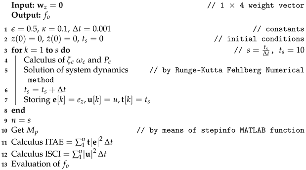
4.4. Quadrotor Subjected to Wind Gust Disturbances

In this section, a Dryden wind gust model is used for the assessment of control robustness. From the set of Equation (4), it is evident that in presence of induced disturbance torques, the angular, as well as the translational trajectory tracking, will be deteriorated. Therefore, in this experiment, the quadrotor is disturbed while it is hovering and path following in order to simulate different scenarios which it would usually face within a wide range of applications. Consider the wind gust mathematical model [39] given by
ξ η ( t ) = d w s + σ = 1 n A σ sin ϖ σ t + φ σ
for η = ϕ , θ , ψ . Expression (46) considers that the disturbance caused by wind field is proportional to the wind speed [39], which is described as a family of time-varying excitations. On the other hand, ϖ σ and φ σ are randomly selected frequencies and phase shifts, respectively; n is the number of sinusoids, A σ is the amplitude, and d w s is a static term for wind disturbance. Thus, the mathematical expression in (46) can be integrated in (5) for this simulation experiment as torque disturbances ξ ϕ , ξ θ and ξ ψ , with n = 6 for ϕ and θ , and n = 7 for ψ . Disturbance parameters are summarized in Table 5.
Consider the following planned references for lateral and longitudinal quadrotor motion in this experiment,
x = 5 cos ( T ) + cos ( 3 T ) cos ( T ) y = 5 sin ( T ) + cos ( 3 T ) sin ( T )
with T = 0.1 t , and the Bézier based motion profile for vertical motion defined by Equations (30) and (52) with the following data: Γ 0 = 0 , Γ f = 5 , T 1 = 2 , T 2 = 10 , T 3 = 57 and T 4 = 65 . Additionally, the yaw motion is regulated about a constant angle ψ = 0 rad. Soft transition between initial condition and the regulation point is accomplished by a Bézier polynomial.
Figure 14 and Figure 15 describes the effective performance of the adaptive robust motion control scheme (20), which compensates the disturbance forces induced by the wind gust model introduced in (46). Moreover, it is evident excellent levels of oscillations attenuation by using our control approach.
From Figure 16, it is observed that the quadrotor is able to efficiently perform trajectory tracking tasks in spite of there is not previous information of the disturbance torques while tracking the planned references introduced in (47). On the other hand, the control input forces and torques generated by the proposed controller are presented in Figure 17. Here, it is appreciated a properly compensation of the disturbance effects which by the computed control inputs. The closed-loop system response for rotational dynamics is plotted in Figure 18, where it is corroborated an efficient performance of the introduced adaptive robust control approach, as done in previous experiments. It is important to mention that during experiment 4 it is adopted the same process for the computation of the control gains in the first experiment.
Finally, in Figure 18, it can be seen the control parameters for rotational motions, which are computed online by means of the adaptive BS-ANN scheme. In addition, it is corroborated that even though there is not available information from derivatives of the angular references, the under-actuation problem is properly solved by the use of the neural networks and the integral reconstructors, thereby a good tracking of the online computed references ϕ and θ is achieved.

4.5. Robustness against Uncertainty of Quadrotor Mass

Another important issue for controlling a quadrotor is the variations of the nominal mass. Notice that the online computed references in (8) which define a proper motion on the plane depends on the nominal mass. Therefore, the quadrotor is supposed to follow the references considering the nominal mass value. Thus, during this experiment, it is probed if the vehicle flight may be deteriorate significantly when an extra mass is added.
Consider the following mass variation for this experiment
m = m n + M Δ t
where m n = 0.973 stands for the nominal quadrotor mass in kg, and M Δ t is an abrupt change of the mass quadrotor described by a modified impulse function given by
M Δ t = 1 2 π σ Δ 2 e t a 2 2 σ Δ 2 + b 0 t < 20.4 1 2 π σ Δ 2 e t c 2 2 σ Δ 2 + d t 20.4
with a = 20.25 , b = 0 , c = 19.55 , d = 0.7 , and σ Δ = 0.4 . During the experiment it is adopted a spiral shape planned reference given by the next parametric equations
x = r cos ( T ) y = r sin ( T )
where
r = 5 + 0.2 cos t
and T = t 6 . Inspecting Figure 19, it is appreciated that the abrupt variation in the quadrotor mass does not affect significantly the following of the planned reference. In Figure 20, it is observed a slightly deviation of the quadrotor angular tracking in contrast with the nominal references θ n and ϕ n , computed with the nominal mass. Moreover, it is evident that after a brief period of time the quadrotor is able to recover from the perturbation and perform a proper tracking of the desired references thanks to the robustness of the proposed control scheme.
In Figure 21a, it is presented the compensation to the mass variation at 20.4 s by the control input u. Figure 21b portrays the vertical motion which is performed before the path following, and is given by the following Bézier polynomial
z = Γ 0 0 t < T 1 Γ 0 + Γ f Γ 0 B z ( t , T 1 , T 2 ) T 1 t < T 2 Γ f t T 2
where Γ 0 = 0 and Γ f = 5 , given in meters, stand for the desired initial and maximum vertical positions. The time values given in seconds are as follows: T 1 = 2 , T 2 = 10 . In addition, B z is the Bézier polynomial introduced in (30) with T i and T f as the initial and final transition times. Moreover, n = 6 , and r 1 = 252 ,   r 2 = 1050 ,   r 3 = 1800 ,   r 4 = 1575 , r 5 = 700 ,   r 6 = 126 .
Future studies will address other methodologies for trajectory generation. Interested readers are referred to [40,41] and references therein for further information on trajectory generation. Moreover, algebraic estimators [42] will be explored for determining variation in the quadrotor nominal mass due to unknown payload and damage or failure in the quadrotor frame.

4.6. Discussion of Results

Throughout the presented experiments in this work, it is corroborated that the introduced control scheme is able to properly leads the quadrotor to stable scenarios in spite of the presence of external forces and torque disturbances, as well as mass uncertainty. Different from the important adaptive robust contributions proposed in [21,22,23], in our approach disturbance observers are unnecessary, only positions measurements are required for motion control, and the use of high frequency discontinuous control actions, as a consequence of the use of signum functions, is avoided. Additionally, due to the low dependency of the quadrotor non-linear mathematical model, the robustness against external disturbances and since it is not required the error derivatives for the implementation of our control scheme, we widely recommend this as an viable strategy for controlling other autonomous systems.

5. Conclusions

A novel adaptive robust neural motion control scheme for quadrotor systems has been introduced in this study. The proposed controller guarantees that the desired trajectory can be tracking by the quadrotor vehicle. The control framework is composited by using dynamic compensators along with an adaptive strategy based on B-spline artificial neural networks. Moreover, an artificial intelligence mechanism based on PSO theory was properly employed for improving the design of the control strategy, as well as the dynamic closed-loop response of the quadrotor system, where ITAE and ISCI metric indexes have been used for measuring the control performance. The introduced research is particularly important because of its potential application in motion tracking control of quadrotor systems, where the use of neither tracking error derivatives nor disturbance observers is required. Several simulation experiments were proposed for purposes of performance and robustness assessment. It was corroborated that, by using the introduced control scheme, the quadrotor dynamic response is sufficiently robust for driving the system to stable scenarios. Vibrating disturbance forces and torques, uncertainty of the quadrotor mass, and wind gusts affecting the quadrotor stable motion were used for testing the control scheme robustness. The suitable integration of adaptive and robust control allows to compensate external disturbances during the quadrotor navigation and soft-motion during take-off and landing. Additionally, the quadrotor performance is improved significantly in contrast when it is adopted fixed values for the control gains. The obtained results, thus, prove that the controlled quadrotor system is able to achieve acceptable control accuracy levels for both trajectory tracking and path following in spite of been subjected to undesired disturbances. Finally, it is worth pointing out that the proposed control strategy can be further extended for the motion control of different autonomous systems subjected to external vibrating disturbances, which will be addressed in future works.

Author Contributions

Research, H.Y.-B., F.B.-C., R.T.-O., A.F.-C., C.S., D.S.; Methodology, H.Y.-B., F.B.-C., R.T.-O., C.S., D.S.; Software, H.Y.-B.; Formal analysis, H.Y.-B., F.B.-C., R.T.-O., A.F.-C.; Supervision, H.Y.-B., F.B.-C., R.T.-O., A.F.-C.; Writing, H.Y.-B., F.B.-C., R.T.-O., A.F.-C., C.S., D.S., Project administration, H.Y.-B. All authors have read and agreed to the published version of the manuscript.

Funding

This research received no external funding.

Institutional Review Board Statement

Not applicable.

Informed Consent Statement

Not applicable.

Data Availability Statement

Not applicable.

Conflicts of Interest

The authors declare no conflict of interest.

References

  1. Castillo, P.; Dzul, A. Aerodynamic Configurations and Dynamic Models. In Unmanned Aerial Vehicles; Lozano, R., Ed.; John Wiley & Sons, Ltd.: Hoboken, NJ, USA, 2013; pp. 1–20. [Google Scholar]
  2. Leutenegger, S.; Hürzeler, C.; Stowers, A.K.; Alexis, K.; Achtelik, M.W.; Lentink, D.; Oh, P.Y.; Siegwart, R. Flying Robots. In Springer Handbook of Robotics; Siciliano, B., Khatib, O., Eds.; Springer International Publishing: Cham, Switzerland, 2016; pp. 623–670. [Google Scholar]
  3. Fahimi, F. Autonomous Helicopters. In Autonomous Robots: Modeling, Path Planning, and Control; Springer: Boston, MA, USA, 2009; pp. 263–317. [Google Scholar]
  4. Gerdes, J.; Holness, A.; Perez-Rosado, A.; Roberts, L.; Greisinger, A.; Barnett, E.; Kempny, J.; Lingam, D.; Yeh, C.H.; Bruck, H.A.; et al. Robo Raven: A Flapping-Wing Air Vehicle with Highly Compliant and Independently Controlled Wings. Soft Robot. 2014, 1, 275–288. [Google Scholar] [CrossRef]
  5. Burri, M.; Gasser, L.; Käch, M.; Krebs, M.; Laube, S.; Ledergerber, A.; Meier, D.; Michaud, R.; Mosimann, L.; Müri, L.; et al. Design and Control of a Spherical Omnidirectional Blimp. In Proceedings of the 2013 IEEE/RSJ International Conference on Intelligent Robots and Systems (IROS), Tokyo, Japan, 3–7 November 2013; pp. 1873–1879. [Google Scholar]
  6. Luque-Vega, L.; Castillo-Toledo, B.; Loukianov, A.G. Robust block second order sliding mode control for a quadrotor. J. Frankl. Inst. 2012, 349, 719–739. [Google Scholar] [CrossRef]
  7. Zhao, J.; Zhang, H.; Li, X. Active disturbance rejection switching control of quadrotor based on robust differentiator. Syst. Sci. Control Eng. 2020, 8, 605–617. [Google Scholar] [CrossRef]
  8. Glida, H.E.; Abdou, L.; Chelihi, A.; Sentouh, C.; Hasseni, S.E.I. Optimal model-free backstepping control for a quadrotor helicopter. Nonlinear Dyn. 2020, 100, 3449–3468. [Google Scholar] [CrossRef]
  9. Pérez-Alcocer, R.; Moreno-Valenzuela, J. A novel Lyapunov-based trajectory tracking controller for a quadrotor: Experimental analysis by using two motion tasks. Mechatronics 2019, 61, 58–68. [Google Scholar] [CrossRef]
  10. Noormohammadi-Asl, A.; Esrafilian, O.; Ahangar Arzati, M.; Taghirad, H.D. System identification and H-based control of quadrotor attitude. Mech. Syst. Signal Process. 2020, 135, 106358. [Google Scholar] [CrossRef]
  11. Huynh, M.Q.; Zhao, W.; Xie, L. 1 adaptive control for quadcopter: Design and implementation. In Proceedings of the 2014 13th International Conference on Control Automation Robotics Vision (ICARCV), Singapore, 10–12 December 2014; pp. 1496–1501. [Google Scholar]
  12. Jafarnejadsani, H.; Sun, D.; Lee, H.; Hovakimyan, N. Optimized L1 Adaptive Controller for Trajectory Tracking of an Indoor Quadrotor. J. Guid. Control Dyn. 2017, 40, 1415–1427. [Google Scholar] [CrossRef]
  13. Erginer, B.; Altuğ, E. Design and implementation of a hybrid fuzzy logic controller for a quadrotor VTOL vehicle. Int. J. Control. Autom. Syst. 2012, 10, 61–70. [Google Scholar] [CrossRef]
  14. Boudjedir, H.; Bouhali, O.; Rizoug, N. Adaptive neural network control based on neural observer for quadrotor unmanned aerial vehicle. Adv. Robot. 2014, 28, 1151–1164. [Google Scholar] [CrossRef]
  15. Eskandarpour, A.; Sharf, I. A constrained error-based MPC for path following of quadrotor with stability analysis. Nonlinear Dyn. 2020, 99, 899–918. [Google Scholar] [CrossRef]
  16. Liu, J. Introduction to Intelligent Control. In Intelligent Control Design and MATLAB Simulation; Springer: Singapore, 2018; pp. 1–5. [Google Scholar]
  17. Dydek, Z.T.; Annaswamy, A.M.; Lavretsky, E. Adaptive Control of Quadrotor UAVs: A Design Trade Study With Flight Evaluations. IEEE Trans. Control Syst. Technol. 2013, 21, 1400–1406. [Google Scholar] [CrossRef]
  18. Sankaranarayanan, V.N.; Roy, S. Introducing switched adaptive control for quadrotors for vertical operations. Optim. Control Appl. Methods 2020, 41, 1875–1888. [Google Scholar] [CrossRef]
  19. Sankaranarayanan, V.N.; Roy, S.; Baldi, S. Aerial Transportation of Unknown Payloads: Adaptive Path Tracking for Quadrotors. In Proceedings of the 2020 IEEE/RSJ International Conference on Intelligent Robots and Systems (IROS), Las Vegas, NV, USA, 25–29 October 2020; pp. 7710–7715. [Google Scholar]
  20. Tian, B.; Cui, J.; Lu, H.; Zuo, Z.; Zong, Q. Adaptive Finite-Time Attitude Tracking of Quadrotors With Experiments and Comparisons. IEEE Trans. Ind. Electron. 2019, 66, 9428–9438. [Google Scholar] [CrossRef]
  21. Nguyen, N.P.; Mung, N.X.; Thanh, H.L.N.N.; Huynh, T.T.; Lam, N.T.; Hong, S.K. Adaptive Sliding Mode Control for Attitude and Altitude System of a Quadcopter UAV via Neural Network. IEEE Access 2021, 9, 40076–40085. [Google Scholar] [CrossRef]
  22. Mehmood, Y.; Aslam, J.; Ullah, N.; Chowdhury, M.S.; Techato, K.; Alzaed, A.N. Adaptive Robust Trajectory Tracking Control of Multiple Quad-Rotor UAVs with Parametric Uncertainties and Disturbances. Sensors 2021, 21, 2401. [Google Scholar] [CrossRef]
  23. Sun, C.; Liu, M.; Liu, C.; Feng, X.; Wu, H. An Industrial Quadrotor UAV Control Method Based on Fuzzy Adaptive Linear Active Disturbance Rejection Control. Electronics 2021, 10, 376. [Google Scholar] [CrossRef]
  24. Yañez-Badillo, H.; Beltran-Carbajal, F.; Tapia-Olvera, R.; Valderrabano-Gonzalez, A.; Favela-Contreras, A.; Rosas-Caro, J.C. A Dynamic Motion Tracking Control Approach for a Quadrotor Aerial Mechanical System. Shock Vib. 2020, 2020, 6635011. [Google Scholar]
  25. Spong, M.; Hutchinson, S.; Vidyasagar, M. Robot Modeling and Control, 2nd ed.; Wiley: Hoboken, NJ, USA, 2020. [Google Scholar]
  26. Fliess, M.; Marquez, R.; Delaleau, E.; Sira-Ramirez, H. Correcteurs proportionnels-intégraux généralisés. ESAIM Control Optim. Calc. Var. 2002, 7, 23–41. [Google Scholar] [CrossRef] [Green Version]
  27. Yao, J.; Deng, W. Active disturbance rejection adaptive control of uncertain nonlinear systems: Theory and application. Nonlinear Dyn. 2017, 89, 1611–1624. [Google Scholar] [CrossRef]
  28. Yañez-Badillo, H.; Tapia-Olvera, R.; Beltran-Carbajal, F. Adaptive Neural Motion Control of a Quadrotor UAV. Vehicles 2020, 2, 468–490. [Google Scholar] [CrossRef]
  29. Brown, M.; Harris, C. Neurofuzzy Adaptive Modelling and Control; Prentice Hall International (UK) Ltd.: Hertfordshire, UK, 1994. [Google Scholar]
  30. Saad, D. (Ed.) On-Line Learning in Neural Networks; Cambridge University Press: New York, NY, USA, 1998. [Google Scholar]
  31. Ravankar, A.; Ravankar, A.A.; Kobayashi, Y.; Hoshino, Y.; Peng, C.C. Path Smoothing Techniques in Robot Navigation: State-of-the-Art, Current and Future Challenges. Sensors 2018, 18, 3170. [Google Scholar] [CrossRef] [PubMed] [Green Version]
  32. Beltran-Carbajal, F.; Tapia-Olvera, R.; Valderrabano-Gonzalez, A.; Yanez-Badillo, H.; Rosas-Caro, J.; Mayo-Maldonado, J. Closed-loop online harmonic vibration estimation in DC electric motor systems. Appl. Math. Model. 2021, 94, 460–481. [Google Scholar] [CrossRef]
  33. Beltran-Carbajal, F.; Silva-Navarro, G. On the algebraic parameter identification of vibrating mechanical systems. Int. J. Mech. Sci. 2015, 92, 178–186. [Google Scholar] [CrossRef]
  34. Conyers, S.A.; Rutherford, M.J.; Valavanis, K.P. An Empirical Evaluation of Ground Effect for Small-Scale Rotorcraft. In Proceedings of the 2018 IEEE International Conference on Robotics and Automation, Brisbane, Australia, 21–26 May 2018; pp. 1244–1250. [Google Scholar]
  35. Li, D.; Zhou, Y.; Shi, Z.; Lu, G. Autonomous landing of quadrotor based on ground effect modelling. In Proceedings of the 2015 34th Chinese Control Conference, Hangzhou, China, 28–30 July 2015; pp. 5647–5652. [Google Scholar]
  36. Marini, F.; Walczak, B. Particle swarm optimization (PSO). A tutorial. Chemom. Intell. Lab. Syst. 2015, 149, 153–165. [Google Scholar] [CrossRef]
  37. Zhao, J.; Li, T.; Qian, J. Application of Particle Swarm Optimization Algorithm on Robust PID Controller Tuning. In Advances in Natural Computation; Wang, L., Chen, K., Ong, Y.S., Eds.; Springer: Berlin/Heidelberg, Germany, 2005; pp. 948–957. [Google Scholar]
  38. Kaminski, M. Neural Network Training Using Particle Swarm Optimization—A Case Study. In Proceedings of the 2019 24th International Conference on Methods and Models in Automation and Robotics (MMAR), Międzyzdroje, Poland, 26–29 August 2019; pp. 115–120. [Google Scholar]
  39. Shi, D.; Wu, Z.; Chou, W. Generalized Extended State Observer Based High Precision Attitude Control of Quadrotor Vehicles Subject to Wind Disturbance. IEEE Access 2018, 6, 32349–32359. [Google Scholar] [CrossRef]
  40. Sreenath, K.; Michael, N.; Kumar, V. Trajectory generation and control of a quadrotor with a cable-suspended load—A differentially-flat hybrid system. In Proceedings of the 2013 IEEE International Conference on Robotics and Automation, Karlsruhe, Germany, 6–10 May 2013; pp. 4888–4895. [Google Scholar]
  41. Mellinger, D.; Kumar, V. Minimum snap trajectory generation and control for quadrotors. In Proceedings of the 2011 IEEE International Conference on Robotics and Automation, Shanghai, China, 9–13 May 2011; pp. 2520–2525. [Google Scholar]
  42. Beltran-Carbajal, F.; Silva-Navarro, G. A fast parametric estimation approach of signals with multiple frequency harmonics. Electr. Power Syst. Res. 2017, 144, 157–162. [Google Scholar] [CrossRef]
Figure 1. Schematic of a non-linear quadrotor system [24].
Mathematics 09 02367 g001
Figure 2. Three layer B-spline artificial neural network structure, Bs-ANN.
Mathematics 09 02367 g002
Figure 3. General structure of the adaptive robust motion control scheme.
Mathematics 09 02367 g003
Figure 4. Cubic Bézier curve defined by a couple of pair of endpoints and control points.
Mathematics 09 02367 g004
Figure 5. Quadrotor navigation on the plane and space.
Mathematics 09 02367 g005
Figure 6. Lateral and longitudinal motion tracking in experiment 1.
Mathematics 09 02367 g006
Figure 7. Vertical motion tracking for experiment 1.
Mathematics 09 02367 g007
Figure 8. Adaptive γ i control parameters, for i = x , y , z .
Mathematics 09 02367 g008
Figure 9. Computed control inputs in experiment 1. (a) Unperturbed. (b) Perturbed.
Mathematics 09 02367 g009
Figure 10. Quadrotor autonomous landing under the ground effect phenomenon: (a) First case. (b) Second case.
Mathematics 09 02367 g010
Figure 11. Time response of a closed-loop controlled second order dynamical system.
Mathematics 09 02367 g011
Figure 12. Tracking motion for experiment 3: (a) First scenario. (b) Second scenario.
Mathematics 09 02367 g012
Figure 13. Fixed and adaptive control parameters used in experiment 3: (a) First scenario. (b) Second scenario.
Mathematics 09 02367 g013
Figure 14. Trajectory tracking for the experiment 4.
Mathematics 09 02367 g014
Figure 15. Path following on the plane for the experiment 4.
Mathematics 09 02367 g015
Figure 16. Translational motion tracking for experiment 4.
Mathematics 09 02367 g016
Figure 17. Computed control inputs in experiment 4.
Mathematics 09 02367 g017
Figure 18. Dynamic rotational closed-loop response for the experiment 4: (a) Computed rotational adaptive control parameters. (b) Angular tracking motion.
Mathematics 09 02367 g018
Figure 19. Simulation results for experiment 5. (a) Path following. (b) Mass variation given by Equation (48).
Mathematics 09 02367 g019
Figure 20. Reference tracking results for experiment 5.
Mathematics 09 02367 g020
Figure 21. Simulation results for experiment 5. (a) Main force control input. (b) Controlled vertical motion.
Mathematics 09 02367 g021
Table 1. Parameters of the 6DOF non-linear quadrotor system.
ParameterUnitsValues
mkg0.98
gm/s29.81
lm0.25
J x kg m20.012450
J y kg m20.012450
J z kg m20.024752
Table 2. Control and endpoint values for the Bézier curves.
SegmentTime Lapse [s] T X 1 Y 1 X 2 Y 2 X 3 Y 3 X 4 Y 4
1 0 t < 10 t 10 00101222
2 10 t < 20 t 10 1 22323444
3 20 t < 30 t 10 2 44545262
4 t 30 t 10 3 62727080
Table 3. Parameters for the adaptive framework in experiment 2.
Case z w 1 , z w 2 , z w 3 , z w 4 , z
First5 × 10 9 1121
Second5 × 10 4 302033
Table 4. Computed ISCI in experiment 3.
Gain CaseISCIITAE
Fixed6.4181 × 10 3 423.9004
Adaptive6.4140 × 10 3 422.9049
Table 5. Values for simulated torque disturbances.
ξ η d w s A 1 A n ϖ 1 ϖ n φ 1 φ n
ξ ϕ 0.3 0.27 , 0.45 , 0.06 , 0.45 , 0.3 , 0.15 π 2.5 , 2 , 0.4 , 0.08 , 0.07 , 0.05 1.2 , 2.7 , 9.5 , 1 , 0.5 , 2
ξ θ 0.6 0.2 , 0.1 , 0.4 , 0.1 , 0.2 , 0.1 π 1.5 , 2 , 0.4 , 0.03 , 0.07 , 0.05 0.3 , 1.7 , 1.5 , 1 , 1.5 , 0.3
ξ ψ 2 0.5 , 0.725 , 1 , 0.5 , 0.25 , 0.5 , 0.25 π 2.5 , 2 , 0.4 , 0.2 , 0.008 , 0.07 , 0.05 3 , 7 , 9.5 , 0 , 1 , 1.5 , 2
Publisher’s Note: MDPI stays neutral with regard to jurisdictional claims in published maps and institutional affiliations.

