An Algebraic Approach for Identification of Rotordynamic Parameters in Bearings with Linearized Force Coefficients

Abstract

In this work, a novel methodology for the identification of stiffness and damping rotordynamic coefficients in a rotor-bearing system is proposed. The mathematical model for the identification process is based on the algebraic identification technique applied to a finite element (FE) model of a rotor-bearing system with multiple degree-of-freedom (DOF). This model considers the effects of rotational inertia, gyroscopic moments, shear deformations, external damping and linear forces attributable to stiffness and damping parameters of the supports. The proposed identifier only requires the system’s vibration response as input data. The performance of the proposed identifier is evaluated and analyzed for both schemes, constant and variable rotational speed of the rotor-bearing system, and numerical results are obtained. In the presented results, it can be observed that the proposed identifier accurately determines the stiffness and damping parameters of the bearings in less than 0.06 s. Moreover, the identification procedure rapidly converges to the estimated values in both tested conditions, constant and variable rotational speed.

1. Introduction

Over the past few decades, several numerical approximations on the dynamic behavior analysis for rotordynamic systems have been developed. Among these approximations, the most popular approach is the finite element (FE) method because it is highly efficient and convenient for modelling diverse physical systems. According to Koutromanos [1], with this method a complex region that defines a continuous system is discretized with simple geometrical forms called finite elements. The material properties as well as the governing relationships are taken into consideration for these elements and expressed in terms of unknown values on the element boundaries. After an assembly process and consideration of the loads and boundary conditions, an equation system is obtained. The solution for these equations provides the approximated behavior of the continuous system. At the start of the 1960s, engineers used the FE method to obtain approximated solutions for problems related to stress analysis, fluid flows, heat transfers and other areas. However, the FE method was not applied to rotordynamics until a decade later. Through the 1970s, diverse efforts were made to incorporate effects of rotational inertia, gyroscopic moments, axial load, shear deformation and internal damping, as pointed out in [2]. Recently, Shen et al. [3] remarked on the importance of including the effects of rotational inertia in the finite elements used to model and analyze rotordynamic systems, in order to have a more general and appropriate kinematic and dynamic description of rotating structures supported by bearings with stiffness and viscous damping characteristics.

Through the bearing characterization in rotor-bearing systems, the rotordynamic stiffness and damping coefficients can be determined. Physical insight of these parameters is essential for the correct modelling of every rotordynamic system as they are important factors in determining the system’s dynamical behavior. In general, when a rotor-bearing system is studied, stiffness and damping coefficients of the bearings are unknown, meaning it is therefore necessary to implement a methodology to determinate them. According to Tiwari [4], Matsushita et al. [5] and Breńkacz [6], there are eight rotordynamic coefficients in bearings, four for stiffness (two directs and two crossed) and four for damping (two directs and two crossed). Nowadays, rotor-bearing systems can be modelled in a very precise way by using modern modelling techniques. However, accurately estimating the dynamic parameters through theoretical models is still a challenge because it is difficult to accurately model every phenomenon affecting the dynamic behavior of the bearings. This problem has led to the development of novel numerical and experimental techniques for dynamic parameter identification [4,6,7]. Tiwari and Chougale [8] developed an algorithm to estimate the dynamic parameters of active magnetic bearings as well as the residual rotor unbalance. The proposed algorithm is based on the least squares technique in frequency domain. Moreover, Xu et al. [9] presented a novel identification approach for estimating bearing dynamic parameters based on the transfer matrix method. Stiffness and damping parameters of an active magnetic bearing were determined by minimizing the error between the unbalance response calculated by the transfer matrix approach and the experimental approach. Mao et al. [10] also proposed a method for identifying bearing dynamic parameters in flexible rotor-bearing systems by minimizing the quadratic error between the numerical and experimental results of the vibration response caused by system unbalance. There are several investigations on methods for identifying unbalance and bearing dynamic parameters [11,12,13,14,15]. Recently, Wang et al. [16] presented the development of algorithms for the simultaneous identification of unbalance and bearing dynamic parameters. In both cases, the proposed algorithms were validated by comparison with experimental data. Additionally, in [17], the authors estimated the rotordynamic coefficients of a controllable floating ring bearing with a magnetorheological fluid (MRF) showing that the magnetic field-induced, field-dependent viscosity of the MRF changes the stiffness and damping bearing coefficients, which can be used to modify the dynamic behavior of the rotor-bearing system. In 2020, Kang et al. [18] used the Kalman filter to estimate the bearing dynamic coefficients of a flexible rotor-bearing system. The rotor system is modeled with Timoshenko beam elements, but the imbalance force considered in the dynamic model is calculated for a constant rotational velocity condition. More recently, in 2021, Chen et al. [19] proposed a method to simultaneously identify the parameters of the oil-film bearings and active magnetic bearings/bearingless motors AMBs/BELMs along with the residual unbalanced forces during the unbalanced vibration of the rotor. The proposed method requires independent rotor responses and control currents to form a regression equation to estimate all of the unknown parameters. Independent rotor responses are realized by changing the PID control parameters of the AMBs/BELMs. The finite element method is used to model the system by using Timoshenko beam elements, and both numerical and experimental results are presented at a unique operation velocity of 2400 rpm. Taherkhani and Ahmadian [20] used the Bayesian approach to an appropriate parameter selection procedure and suitable sampling strategy for stochastic model updating to investigate variability in the dynamic behavior of a complex turbo compressor supported by hydrodynamic bearings, leading to successful parameter identification results. Brito Jr. et al. [21] presented an experimental method to estimate the direct and cross-coupled dynamic coefficients of tilting-pad journal bearings of vertical hydro-generators. The method employs only the shaft radial relative vibrations, and the bearing radial absolute vibrations originated by the hydro-generator residual unbalance. The authors affirmed that the vibration measurements required by the estimation method could be a major problem in low-speed machines (less than 400 rpm). Although any type of bearing provides stiffness and damping forces that may depend on the operation speed and many other factors, linearized force coefficients are widely used to model the reaction forces from fluid film bearings. These linear force coefficients are derived from the assumption of small amplitude motions about an equilibrium position [22] and have been used to study the dynamic responses and analyze the stability of rotor systems supported by oil-lubricated tilting-pad bearings, cylindrical bearings and foil bearings, as pointed out in [23] and references within. Recently, Dyk et al. [24] presented diverse linearization methods in the stability analysis of rotating systems supported on floating ring bearing (FRBs), demonstrating the usefulness of the linear force coefficients to predict the dynamic behavior of non-linear systems such as turbochargers supported by FRBs.

There is also substantial literature on parameter identification and estimation methods. Most of these schemes are essentially asymptotic, recursive or complex [25,26,27], and, according to Arias-Montiel et al. [28], these methods lead to unrealistic implementations. Over the past few years, another method of parametric identification called algebraic identification has been successfully implemented in a wide range of engineering applications [29]. The algebraic identification method is based on differential algebra and operational calculus for developing estimators in determining unknown system parameters from a mathematical model. These estimations are carried out on-line in continuous or discrete time. An advantage of algebraic identification over other methods is that it provides identification expressions that are completely independent of the initial system conditions. Algebraic identification has been used for parameter and signal estimation in linear and non-linear vibrational mechanical systems [30,31,32,33,34,35,36,37,38,39]. Numerical and experimental results show that algebraic identification is extremely robust against parameter uncertainty, frequency variations, measurement errors and signal noise. Additional information on the algebraic identification robustness and other advantages and disadvantages of this method are highlighted by Sira-Ramírez et al. in [29].

In this work, a novel methodology for developing two mathematical models for identifying the unknown stiffness and damping parameters of bearings in multiple degree-of-freedom (DOF) rotor-bearing systems is proposed. This methodology is based on the algebraic identification technique. Developed identifiers are obtained based on an FE model for a multiple DOF rotor-bearing system that considers the effects of rotational inertia, gyroscopic effects, shear deformations, internal damping and linear forces attributable to stiffness and damping parameters of the supports. Estimators are developed for two different operation conditions of the rotor-bearing system: constant and variable rotational speed. Analysis and evaluation of the proposed identifiers is carried out by numerical results showing the viability for applying algebraic identification techniques for the rotordynamic coefficients in rotor-bearing systems.

2. Materials and Methods

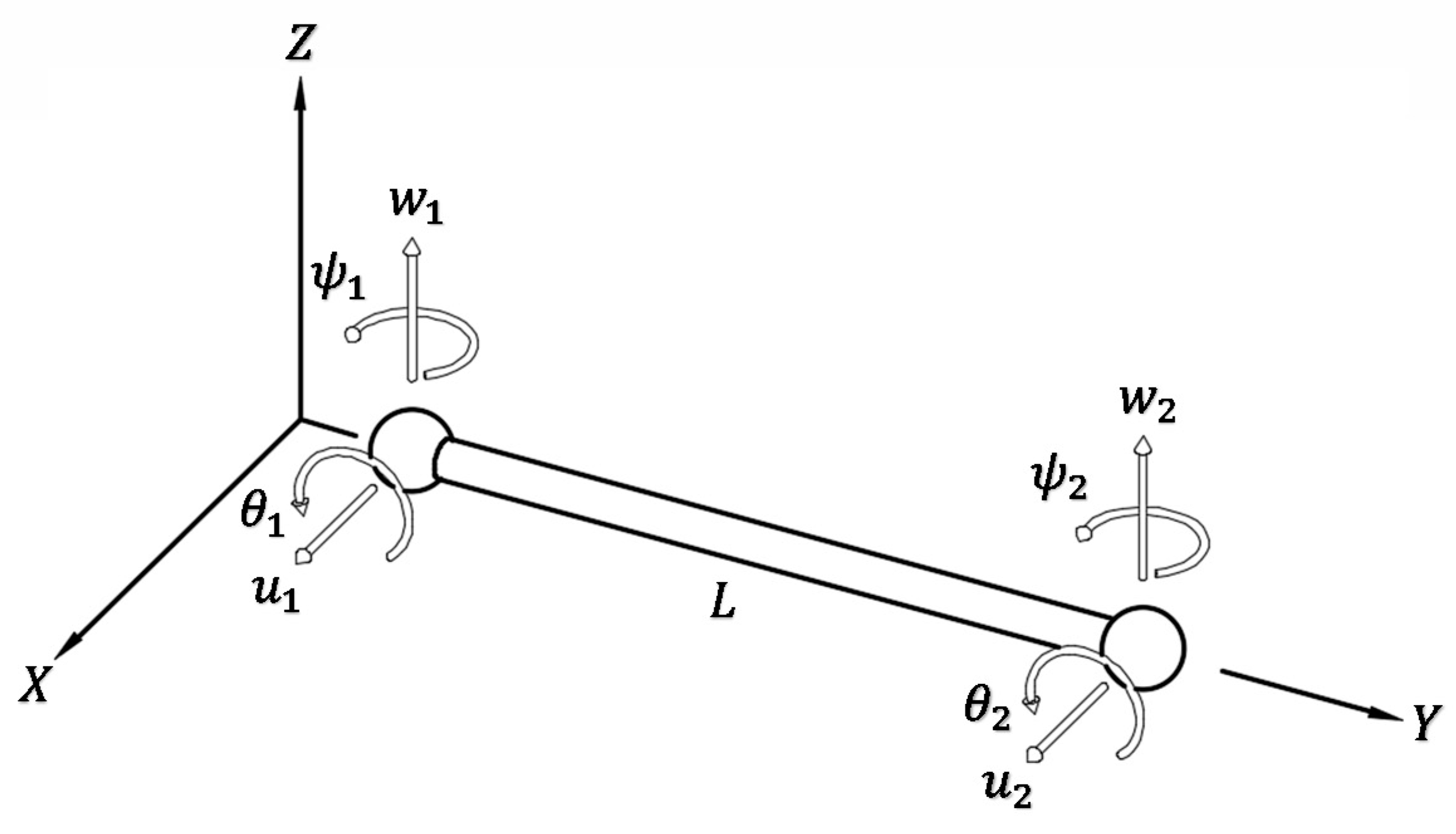
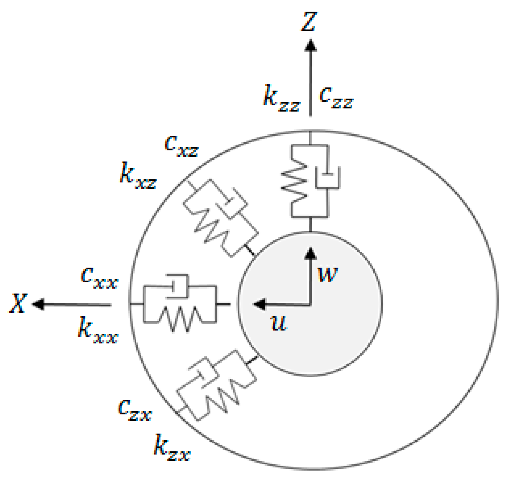
2.1. Mathematical Model of the Rotor-Bearing System

The FE method is used to obtain the mathematical model of the multiple DOF rotor-bearing system. The shaft is modelled with a finite element type beam with four DOF per node, two lateral displacements and two rotations (beam deflections), as illustrated in Figure 1.

The nodal displacement vector is defined as

$$\left\{\delta \right\}={\left\{u_1,w_1,{\psi }_1,{\theta }_1,u_2,w_2,{\psi }_2,{\theta }_2\right\}}^T$$

(1)

where superscript T denotes the transposed vector.

Displacement and rotations corresponding to the movement along X and Z directions are

$$\begin{gathered} \left\{{\delta }_u\right\}={\left\{u_1,{\psi }_1,u_2,{\psi }_2\right\}}^T \\ \left\{{\delta }_w\right\}={\left\{w_1,{\theta }_1,w_2,{\theta }_2\right\}}^T \end{gathered}$$

(2)

The mathematical model of the multiple DOF rotor-bearing system with excitation by unbalanced mass is given by [2]

$$\left[M\right]\left\{\ddot{\delta }\right\}+\left[C\left(\dot{\varphi }\right)\right]\left\{\dot{\delta }\right\}+\left[K\left(\ddot{\varphi }\right)\right]\left\{\delta \right\}={\dot{\varphi }}^2\left\{F_{u\left(1\right)}\left(\varphi \right)\right\}+\ddot{\varphi }\left\{F_{u\left(2\right)}\left(\varphi \right)\right\}$$

(3)

with

$$\begin{gathered} F_{u\left(1\right)}=m_{u}d\left(\sin \left(\varphi +\alpha \right)+\cos \left(\varphi +\alpha \right)\right) \\ {F}_{u\left(2\right)}=m_{u}d\left(\sin \left(\varphi +\alpha \right)-\cos \left(\varphi +\alpha \right)\right) \end{gathered}$$

where $m_u$, $d$ and $\alpha$, are mass, eccentricity and angular position of system unbalance, respectively, $\ddot{\varphi }$ and $\dot{\varphi }$ are angular acceleration and velocity of the rotor-bearing system, respectively, and $\varphi =\dot{\varphi }t$. Moreover, $\left\{\delta \right\}$ is a vector with all the nodal displacements, $\left[M\right]$ is the global mass matrix of the system, $\left[C\left(\dot{\varphi }\right)\right]$ is the global damping matrix that includes gyroscopic effects as a function of the rotational velocity $\left(\dot{\varphi }\left[C_2\right]\right)$ and $\left[C_1\right]$ that represents the damping in the supports, $\left[K\left(\ddot{\varphi }\right)\right]$ is the global stiffness matrix constituted by $\left[K_1\right], \left[K_2\right]$, which include the supports and rotor stiffness, respectively, and $\ddot{\varphi }\left[K_3\right]$, which is a stiffness term as a function of the rotational acceleration of the system. Finally, $\left\{F_{u\left(1\right)}\left(\varphi \right)\right\}$ and $\left\{F_{u\left(2\right)}\left(\varphi \right)\right\}$ are the components of the centrifugal force vector caused by the unbalanced mass. Shape functions for the beam type finite element and a detailed definition for matrices in Equation (3) are provided in Appendix A.

Stiffness and damping matrices provided by the bearings are obtained by determining the generalized forces that these elements exert on the rotor shaft. After applying the virtual work principle to the bearing model shown in Figure 2, forces acting on the rotor can be expressed in a matrix form as [40]

$$\left\{\begin{array}{c}{F}_{u_i}\\ F_{w_i}\end{array}\right\}=-\left[\begin{array}{c}{k}_{xx}\\ k_{zx}\end{array} \begin{array}{c}{k}_{xz}\\ k_{zz}\end{array}\right]\left\{\begin{array}{c}{u}_i\\ w_i\end{array}\right\}-\left[\begin{array}{c}{c}_{xx}\\ c_{zx}\end{array} \begin{array}{c}{c}_{xz}\\ c_{zz}\end{array}\right]\left\{\begin{array}{c}{\dot{u}}_i\\ {\dot{w}}_i\end{array}\right\}$$

(4)

where $i$ denotes the nodal location of the bearing inside the rotordynamic systems. Matrices from the right side of Equation (4) are stiffness and damping matrices corresponding to system supports $\left[K_1\right]$ and $\left[C_1\right]$, respectively.

2.2. Operation Velocity of the Rotor-Bearing System

Two different conditions for the operation velocity of the rotor-bearing system are considered: constant velocity and a linear ramp excitation.

Under the constant velocity scheme, no time variation of the rotating machine excitation is considered. This condition can be expressed as

$$\dot{\varphi }\left(t\right)=\mathsf{\Omega }=\mathrm{constant}$$

(5)

The term “ramp excitation” means a continuous variation in the excitation frequency with a specific ratio with respect to time and can be ascendant (up) or descendent (down). With most real rotating systems, the excitation frequency does not change in a linear manner with respect to time. However, in some cases, frequency variation is sufficiently slow to be approximated by a linear function. For the solution of Equation (3), it is considered a variation of the excitation frequency of the form

$$\dot{\varphi }\left(t\right)={\dot{\varphi }}_0+\ddot{\varphi t}$$

(6)

where:

• ${\dot{\varphi }}_0$ is the excitation frequency at the ramp beginning;
• $\ddot{\varphi }$ is the change ratio with respect to time of the excitation frequency;
• t is the time.

2.3. Mathematical Model for Bearing Rotordynamic Parameters Identification

The development of the mathematical model of the identifier is carried out from the rotordynamic system model given in Equation (3), considering both cases: constant and variable system operation velocity.

2.3.1. Algebraic Identifier with Constant Operation Velocity

As pointed out above, it is necessary to have a mathematical model for the dynamic behavior of the rotor-bearing system to develop algebraic identifiers. From this model and through an algebraic manipulation of the equations, estimators for the unknown parameters are obtained.

If a constant rotational velocity of the system is considered, Equation (3) can be written as

$$\left[M\right]\left\{\ddot{\delta }\right\}+\left[C_1+\mathsf{\Omega }{C}_2\right]\left\{\dot{\delta }\right\}+\left[K_1+K_2\right]\left\{\delta \right\}=m_{u}d{\mathsf{\Omega }}^2\left\{\sin \left(\mathsf{\Omega }\mathrm{t}+\mathsf{\alpha }\right)+\cos \left(\mathsf{\Omega }\mathrm{t}+\mathsf{\alpha }\right)\right\}$$

(7)

Now, Equation (7) is multiplied by $t^2$ and, after that, the result is twice integrated with respect to time, giving

$$\begin{gathered} {{\displaystyle \int }}^{\left(2\right)}\left[K_1\right]t^2\left\{\delta \right\}+\left[C_1\right]\left[{{\displaystyle \int }}^{ }{t}^2\left\{\delta \right\}-2{{\displaystyle \int }}^{\left(2\right)}t\left\{\delta \right\}\right] \\ ={{\displaystyle \int }}^{\left(2\right)}{m}_{u}d{\mathsf{\Omega }}^2\left\{\sin \left(\mathsf{\Omega }\mathrm{t}+\mathsf{\alpha }\right)+\cos \left(\mathsf{\Omega }\mathrm{t}+\mathsf{\alpha }\right)\right\}{t}^2 \end{gathered}$$

(8)

where ${{\displaystyle \int }}^{\left(2\right)}f\left(t\right)$ denotes iterated integrals. Furthermore, bearing stiffness and damping terms to be identified are included in $\left[K_1\right]$ and $\left[C_1\right]$, respectively. Therefore, after the integration of the left side of Equation (8) and an algebraic treatment, the following expression can be obtained

$$\begin{gathered} {{\displaystyle \int }}^{\left(2\right)}\left[\left[M\right]\left\{\ddot{\delta }\right\}+\left[C_1+\mathsf{\Omega }{C}_2\right]\left\{\dot{\delta }\right\}+\left[K_1+K_2\right]\left\{\delta \right\}\right]t^2 \\ ={{\displaystyle \int }}^{\left(2\right)}\left[2\mathsf{\Omega }{C}_{2}t-2M-K_2{t}^2\right]\left\{\delta \right\}+{{\displaystyle \int }}^{ }\left[4M-\mathsf{\Omega }{C}_{2}t\right]t\left\{\delta \right\} \\ -\left\{M\right\}{t}^2\left\{\delta \right\}+{{\displaystyle \int }}^{\left(2\right)}{m}_{u}d{\mathsf{\Omega }}^2\left\{\sin \left(\mathsf{\Omega }\mathrm{t}+\mathsf{\alpha }\right)+\cos \left(\mathsf{\Omega }\mathrm{t}+\mathsf{\alpha }\right)\right\}{t}^2 \end{gathered}$$

(9)

Equation (9) can be separated into individual equation systems for each node where the bearings are located. These equations can be presented in the form

$$\left[\begin{array}{cc}{k}_{xx}& k_{xz}\\ k_{zx}& k_{zz}\end{array}\right] {{\displaystyle \int }}^{\left(2\right)}{t}^2\left\{\begin{array}{c}{u}_i\\ w_i\end{array}\right\}+\left[\begin{array}{cc}{c}_{xx}& c_{xz}\\ c_{zx}& c_{zz}\end{array}\right]\left({{\displaystyle \int }}^{ }{t}^2\left\{\begin{array}{c}{u}_i\\ w_i\end{array}\right\}-2{{\displaystyle \int }}^{\left(2\right)}t\left\{\begin{array}{c}{u}_i\\ w_i\end{array}\right\}\right)=\left\{\begin{array}{c}{b}_{ui}\\ b_{wi}\end{array}\right\}$$

(10)

To solve Equation (10) an equal number of equations and unknowns is needed. For this, Equation (10) is successively integrated three times in order to obtain the missing equations, which are written as

$$\left[\begin{array}{cc}{k}_{xx}& k_{xz}\\ k_{zx}& k_{zz}\end{array}\right] {{\displaystyle \int }}^{\left(3\right)}{t}^2\left\{\begin{array}{c}{u}_i\\ w_i\end{array}\right\}+\left[\begin{array}{cc}{c}_{xx}& c_{xz}\\ c_{zx}& c_{zz}\end{array}\right]\left({{\displaystyle \int }}^{\left(2\right)}{t}^2\left\{\begin{array}{c}{u}_i\\ w_i\end{array}\right\}-2{{\displaystyle \int }}^{\left(3\right)}t\left\{\begin{array}{c}{u}_i\\ w_i\end{array}\right\}\right)={\displaystyle \int }\left\{\begin{array}{c}{b}_{ui}\\ b_{wi}\end{array}\right\}$$

(11)

$$\left[\begin{array}{cc}{k}_{xx}& k_{xz}\\ k_{zx}& k_{zz}\end{array}\right] {{\displaystyle \int }}^{\left(4\right)}{t}^2\left\{\begin{array}{c}{u}_i\\ w_i\end{array}\right\}+\left[\begin{array}{cc}{c}_{xx}& c_{xz}\\ c_{zx}& c_{zz}\end{array}\right]\left({{\displaystyle \int }}^{\left(3\right)}{t}^2\left\{\begin{array}{c}{u}_i\\ w_i\end{array}\right\}-2{{\displaystyle \int }}^{\left(4\right)}t\left\{\begin{array}{c}{u}_i\\ w_i\end{array}\right\}\right)={{\displaystyle \int }}^{\left(2\right)}\left\{\begin{array}{c}{b}_{ui}\\ b_{wi}\end{array}\right\}$$

(12)

$$\left[\begin{array}{cc}{k}_{xx}& k_{xz}\\ k_{zx}& k_{zz}\end{array}\right] {{\displaystyle \int }}^{\left(5\right)}{t}^2\left\{\begin{array}{c}{u}_i\\ w_i\end{array}\right\}+\left[\begin{array}{cc}{c}_{xx}& c_{xz}\\ c_{zx}& c_{zz}\end{array}\right]\left({{\displaystyle \int }}^{\left(4\right)}{t}^2\left\{\begin{array}{c}{u}_i\\ w_i\end{array}\right\}-2{{\displaystyle \int }}^{\left(5\right)}t\left\{\begin{array}{c}{u}_i\\ w_i\end{array}\right\}\right)={{\displaystyle \int }}^{\left(3\right)}\left\{\begin{array}{c}{b}_{ui}\\ b_{wi}\end{array}\right\}$$

(13)

From Equations (10)–(13), a linear system equation is obtained for each node where the bearings are located. These equations can be expressed as

$$\left[A_s\left(t\right)\right]\left\{{\mathsf{\Theta }}_s\right\}=\left\{b_s\left(t\right)\right\}$$

(14)

where $\left\{{\mathsf{\Theta }}_s\right\}={\left\{k_{xx} k_{xz} k_{zx} k_{zz} c_{xx} c_{xz} c_{zx} c_{zz} \right\}}^T$ denotes the transposed vector of parameters to be identified and $\left[A_s\left(t\right)\right], \left\{b_s\left(t\right)\right\}$ are 8 × 8 and 8 × 1, respectively.

As can be observed in Figure 2, eight parameters are required to define stiffness and damping characteristics provided by the system supports. This is because in order to obtain the terms of $\left[A_s\left(t\right)\right]$ and $\left\{b_s\left(t\right)\right\}$ in Equation (14), eight simultaneous equations involving the unknown support parameters are required to obtain their magnitudes.

From Equation (14) it can be concluded that vector $\left\{{\mathsf{\Theta }}_s\right\}$ is identifiable if, and only if, the dynamic system trajectory is persistent. That is to say, the trajectories or dynamic system behaviors satisfy the condition $det\left[A_s\left(t\right)\right]\ne 0$. In general, this condition is maintained at least in a small interval $(t_0,t_0+ϵ]$ where $ϵ$ is a positive and sufficiently small value [29]. Then, the linear system Equation (14) is solved to obtain the algebraic identifier for determining the stiffness and damping parameters of rotor-bearing support with constant operation velocity.

$$\left\{{\mathsf{\Theta }}_s\right\}={\left[{\mathrm{A}}_s\right]}^{-1}\left\{b_s\right\} \forall t\in (t_0,t_0+ϵ].$$

(15)

It is important to mention that to identify the support parameters, lateral vibration measurements at the node and the nodal slopes are required. Moreover, similar information from the adjacent node is also needed. The nodal slopes can be calculated by numerical approximation using the lateral displacements from two adjacent nodes.

2.3.2. Algebraic Identifier with Variable Operation Velocity

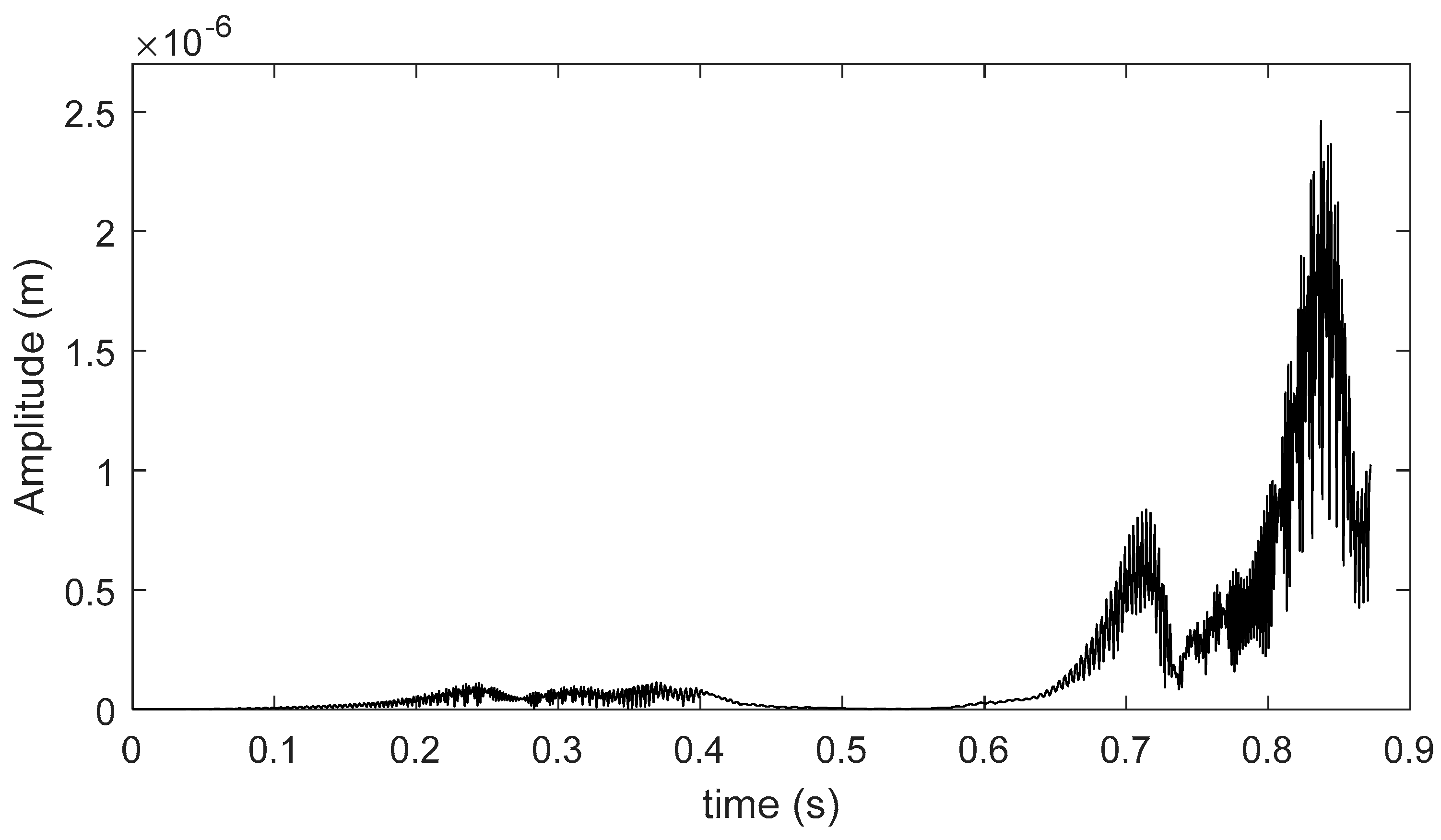
In this section, the rotor-bearing system velocity is considered as a linear ramp of excitation. The mathematical model of the system is defined by Equation (3). In order to develop the parameter identifier, this equation is rewritten as follows

$$\left[M\right]\left\{\ddot{\delta }\right\}+\left[C_1+\dot{\varphi }{C}_2\right]\left\{\dot{\delta }\right\}+\left[K_1+K_2+\ddot{\varphi }{K}_3\right]\left\{\delta \right\}={\dot{\varphi }}^2{F}_1\left(\varphi \right)+\ddot{\varphi }{F}_2\left(\varphi \right)$$

(16)

By multiplying Equation (16) by $t^2$ and integrating the result twice with respect to time, the following is obtained

$$\begin{gathered} {{\displaystyle \int }}^{\left(2\right)}\left[\left[M\right]\left\{\ddot{\delta }\right\}+\left[C_1+\dot{\varphi }{C}_2\right]\left\{\dot{\delta }\right\}+\left[K_1+K_2+\ddot{\varphi }{K}_3\right]\left\{\delta \right\}\right]t^2 \\ ={{\displaystyle \int }}^{\left(2\right)}\left\{{\dot{\varphi }}^2{F}_1\left(\varphi \right)+\ddot{\varphi }{F}_2\left(\varphi \right)\right\}{t}^2 \end{gathered}$$

(17)

where ${{\displaystyle \int }}^{\left(2\right)}\phi \left(t\right)$ are iterated time-integrals of the form ${{\displaystyle \int }}_0^t{{\displaystyle \int }}_0^{{\sigma }_1}\cdots {{\displaystyle \int }}_0^{{\sigma }_{n-1}}\phi \left({\sigma }_n\right)d{\sigma }_n\cdots d{\sigma }_1$ with ${{\displaystyle \int }}^{ }\phi \left(t\right)={{\displaystyle \int }}_0^t\phi \left(\sigma \right)d\sigma$, and $n$ a positive integer.

Similarly for the case of constant velocity, matrices $\left[K_1\right]$ and $\left[C_1\right]$ contain the stiffness and damping parameters provided by the supports. Therefore, after the integration of the left part of Equation (17) and rearranging terms, we have

$$\begin{gathered} {{\displaystyle \int }}^{\left(2\right)}{\left[K\right]}_1{t}^2\left\{\delta \right\}+\left[C_1\right]\left[{{\displaystyle \int }}^{ }{t}^2\left\{\delta \right\}-2{{\displaystyle \int }}^{\left(2\right)}t\left\{\delta \right\}\right]={{\displaystyle \int }}^{ }\left[4Mt-\dot{\varphi }{C}_2{t}^2\right]\left\{\delta \right\} \\ +{{\displaystyle \int }}^{\left(2\right)}\left[C_2\left(\ddot{\varphi }{t}^2+2\dot{\varphi }t\right)-2M-\left(K_2+\ddot{\varphi }{K}_3\right)t^2\right]\left\{\delta \right\}-\left[M\right]t^2\left\{\delta \right\} \\ +{{\displaystyle \int }}^{\left(2\right)}\left\{{\dot{\varphi }}^2{F}_1\left(\varphi \right)+\ddot{\varphi }{F}_2\left(\varphi \right)\right\}{t}^2 \end{gathered}$$

(18)

It is worth mentioning that Equation (18) can be separated into individual equation systems for each node where the bearings are located. These equations can be written as follows

$$\left[\begin{array}{cc}{k}_{xx}& k_{xz}\\ k_{zx}& k_{zz}\end{array}\right] {{\displaystyle \int }}^{\left(2\right)}{t}^2\left\{\begin{array}{c}{u}_i\\ w_i\end{array}\right\}+\left[\begin{array}{cc}{c}_{xx}& c_{xz}\\ c_{zx}& c_{zz}\end{array}\right]\left({{\displaystyle \int }}^{ }{t}^2\left\{\begin{array}{c}{u}_i\\ w_i\end{array}\right\}-2{{\displaystyle \int }}^{\left(2\right)}t\left\{\begin{array}{c}{u}_i\\ w_i\end{array}\right\}\right)=\left\{\begin{array}{c}{b}_{ui}\\ b_{wi}\end{array}\right\}$$

(19)

To solve Equation (19), an equal number of equations and unknows is required. Therefore, Equation (19) is successively integrated three times to obtain the missing equations which are expressed as

$$\left[\begin{array}{cc}{k}_{xx}& k_{xz}\\ k_{zx}& k_{zz}\end{array}\right] {{\displaystyle \int }}^{\left(3\right)}{t}^2\left\{\begin{array}{c}{u}_i\\ w_i\end{array}\right\}+\left[\begin{array}{cc}{c}_{xx}& c_{xz}\\ c_{zx}& c_{zz}\end{array}\right]\left({{\displaystyle \int }}^{\left(2\right)}{t}^2\left\{\begin{array}{c}{u}_i\\ w_i\end{array}\right\}-2{{\displaystyle \int }}^{\left(3\right)}t\left\{\begin{array}{c}{u}_i\\ w_i\end{array}\right\}\right)={\displaystyle \int }\left\{\begin{array}{c}{b}_{ui}\\ b_{wi}\end{array}\right\}$$

(20)

$$\left[\begin{array}{cc}{k}_{xx}& k_{xz}\\ k_{zx}& k_{zz}\end{array}\right] {{\displaystyle \int }}^{\left(4\right)}{t}^2\left\{\begin{array}{c}{u}_i\\ w_i\end{array}\right\}+\left[\begin{array}{cc}{c}_{xx}& c_{xz}\\ c_{zx}& c_{zz}\end{array}\right]\left({{\displaystyle \int }}^{\left(3\right)}{t}^2\left\{\begin{array}{c}{u}_i\\ w_i\end{array}\right\}-2{{\displaystyle \int }}^{\left(4\right)}t\left\{\begin{array}{c}{u}_i\\ w_i\end{array}\right\}\right)={{\displaystyle \int }}^{\left(2\right)}\left\{\begin{array}{c}{b}_{ui}\\ b_{wi}\end{array}\right\}$$

(21)

$$\left[\begin{array}{cc}{k}_{xx}& k_{xz}\\ k_{zx}& k_{zz}\end{array}\right] {{\displaystyle \int }}^{\left(5\right)}{t}^2\left\{\begin{array}{c}{u}_i\\ w_i\end{array}\right\}+\left[\begin{array}{cc}{c}_{xx}& c_{xz}\\ c_{zx}& c_{zz}\end{array}\right]\left({{\displaystyle \int }}^{\left(4\right)}{t}^2\left\{\begin{array}{c}{u}_i\\ w_i\end{array}\right\}-2{{\displaystyle \int }}^{\left(5\right)}t\left\{\begin{array}{c}{u}_i\\ w_i\end{array}\right\}\right)={{\displaystyle \int }}^{\left(3\right)}\left\{\begin{array}{c}{b}_{ui}\\ b_{wi}\end{array}\right\}$$

(22)

From Equations (19)–(22), a linear system equation is obtained for each node where the bearings are located. These equations can be expressed as

$$\left[A_s\left(t\right)\right]\left\{{\mathsf{\Theta }}_s\right\}=\left\{b_s\left(t\right)\right\}$$

(23)

where $\left\{{\mathsf{\Theta }}_s\right\}={\left\{k_{xx} k_{xz} k_{zx} k_{zz} c_{xx} c_{xz} c_{zx} c_{zz} \right\}}^T$ denotes the transposed vector of parameters to be identified and $\left[A_s\left(t\right)\right], \left\{b_s\left(t\right)\right\}$ are 8 × 8 and 8 × 1, respectively.

Again, the condition $det\left[A_s\left(t\right)\right]\ne 0$ must be satisfied to identify the vector $\left\{{\mathsf{\Theta }}_s\right\}$.

From the solution of Equation (23), a mathematical model for an on-line identifier of stiffness and damping bearing parameters can be obtained as

$$\left\{{\mathsf{\Theta }}_s\right\}=\left[A_s{}^{-1}\right]\left\{b_s\right\} \forall t\in (t_0,t_0+ϵ]$$

(24)

As can be observed, algebraic identification of stiffness and damping bearing parameters is independent of system initial conditions and only depends on the displacement vector and the type of ramp excitation. It is important to mention that as with the case of constant velocity, to identify the supports parameters, lateral vibration measurements at the node and the nodal slopes are required. Moreover, similar information from the adjacent node is also needed.

3. Results

In Figure 3, a scheme of the rotor-bearing system considered in this work and its discretization is presented.

To obtain the mathematical model for the rotor-bearing system using the FE method, it was discretized into 11 beam-like elements, as is shown in Figure 3. The system includes two inertial disks located at nodes 1 and 12, while supports (bearings) are placed at nodes 4 and 8. The correct nodal location ensures that the simulation replicates the model’s real conditions. In addition, two unbalanced masses were considered in two different angular positions located on inertial disks $D_1$ and $D_2$.

In

Table 1. Mechanical and geometrical properties of the rotor-bearing shaft.

Parameter	Value	Parameter	Value
Modulus of elasticity	$2\times {10}^{11} \mathrm{N}/{\mathrm{m}}^2$	$L_1$	$0.035 \mathrm{m}$
Density	$7800 \mathrm{kg}/{\mathrm{m}}^3$	$L_2$	$0.010 \mathrm{m}$
Poisson ratio	$0.3$	$L_3$	$0.025 \mathrm{m}$
$r_1$	$0.005 \mathrm{m}$	$L_4$	$0.130 \mathrm{m}$
$r_2$	$0.02 \mathrm{m}$	$L_5$	$0.050 \mathrm{m}$
$r_3$	$0.035 \mathrm{m}$	$L_6$	$0.050 \mathrm{m}$

, the mechanical and geometrical properties of the shaft are shown, while the inertial properties of discs and unbalanced masses are presented in

Table 2. Inertial properties of the disks and unbalance masses.

Parameter	Value	Parameter	Value
$D_1$ mass	$1.2 \mathrm{kg}$	$D_2$ mass	$1.0 \mathrm{kg}$
$D_1$ moment of inertia	$1.2\times {10}^{-3} \mathrm{kg}·{\mathrm{m}}^2$	$D_2$ moment of inertia	$1.0\times {10}^{-3} \mathrm{kg}·{\mathrm{m}}^2$
$D_1$ polar moment of inertia	$2.4\times {10}^{-3} \mathrm{kg}·{\mathrm{m}}^2$	$D_2$ polar moment of inertia	$2.0\times {10}^{-3 }\mathrm{kg}·{\mathrm{m}}^2$
$D_1$ mass unbalance	$5\times {10}^{-7} \mathrm{kg}·\mathrm{m} \angle 0 rad$	$D_2$ mass unbalance	$5\times {10}^{-7} \mathrm{kg}·\mathrm{m} \angle \pi rad$

.

In

Table 3. Stiffness and damping bearing parameters [40].

Parameter	Bearing 1 (Node 4)	Bearing 2 (Node 8)
$k_{xx}$	$8\times {10}^7 \mathrm{N}/\mathrm{m}$	$5\times {10}^7 \mathrm{N}/\mathrm{m}$
$k_{xz}$	$-1\times {10}^7 \mathrm{N}/\mathrm{m}$	$-2\times {10}^7 \mathrm{N}/\mathrm{m}$
$k_{zx}$	$-6\times {10}^7 \mathrm{N}/\mathrm{m}$	$-4\times {10}^7 \mathrm{N}/\mathrm{m}$
$k_{zz}$	$1\times {10}^8 \mathrm{N}/\mathrm{m}$	$7\times {10}^7\mathrm{N}/\mathrm{m}$
$c_{xx}$	$8\times {10}^3 \mathrm{N}·\mathrm{s}/\mathrm{m}$	$6\times {10}^3 \mathrm{N}·\mathrm{s}/\mathrm{m}$
$c_{xz}$	$-3\times {10}^3 \mathrm{N}·\mathrm{s}/\mathrm{m}$	$-1.5\times {10}^3 \mathrm{N}·\mathrm{s}/\mathrm{m}$
$c_{zx}$	$-3\times {10}^3 \mathrm{N}·\mathrm{s}/\mathrm{m}$	$-1.5\times {10}^3 \mathrm{N}·\mathrm{s}/\mathrm{m}$
$c_{zz}$	$1.2\times {10}^4 \mathrm{N}·\mathrm{s}/\mathrm{m}$	$8\times {10}^3 \mathrm{N}·\mathrm{s}/\mathrm{m}$

, the stiffness and damping bearing parameters [40] used for numerical simulation are presented.

On-line algebraic identification of stiffness and damping bearing parameters was determined based on the vibratory response of the rotor-bearing system in the time domain, which was obtained from Equations (3) and (7) by using the Newmark method for numerical integration.

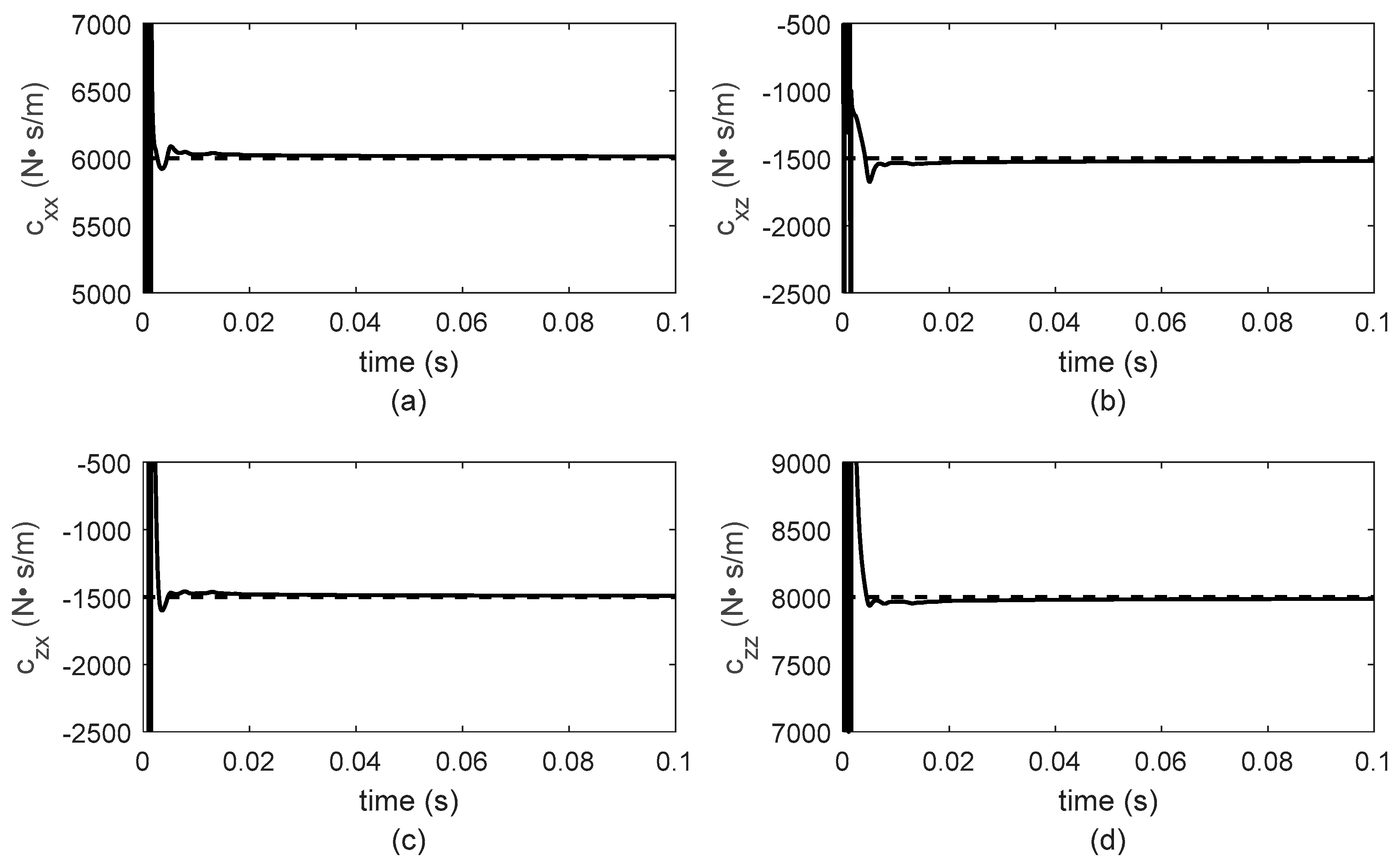
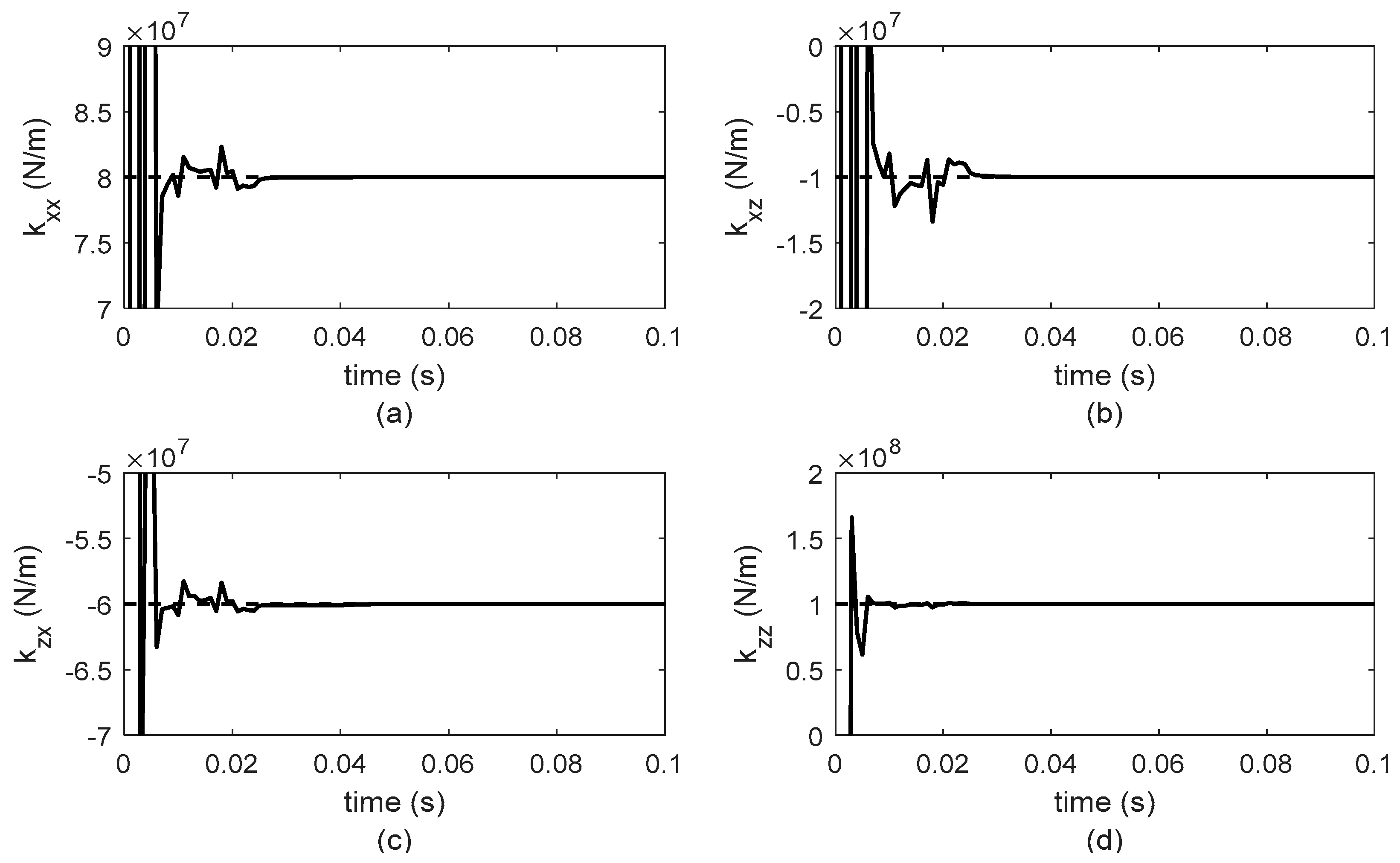
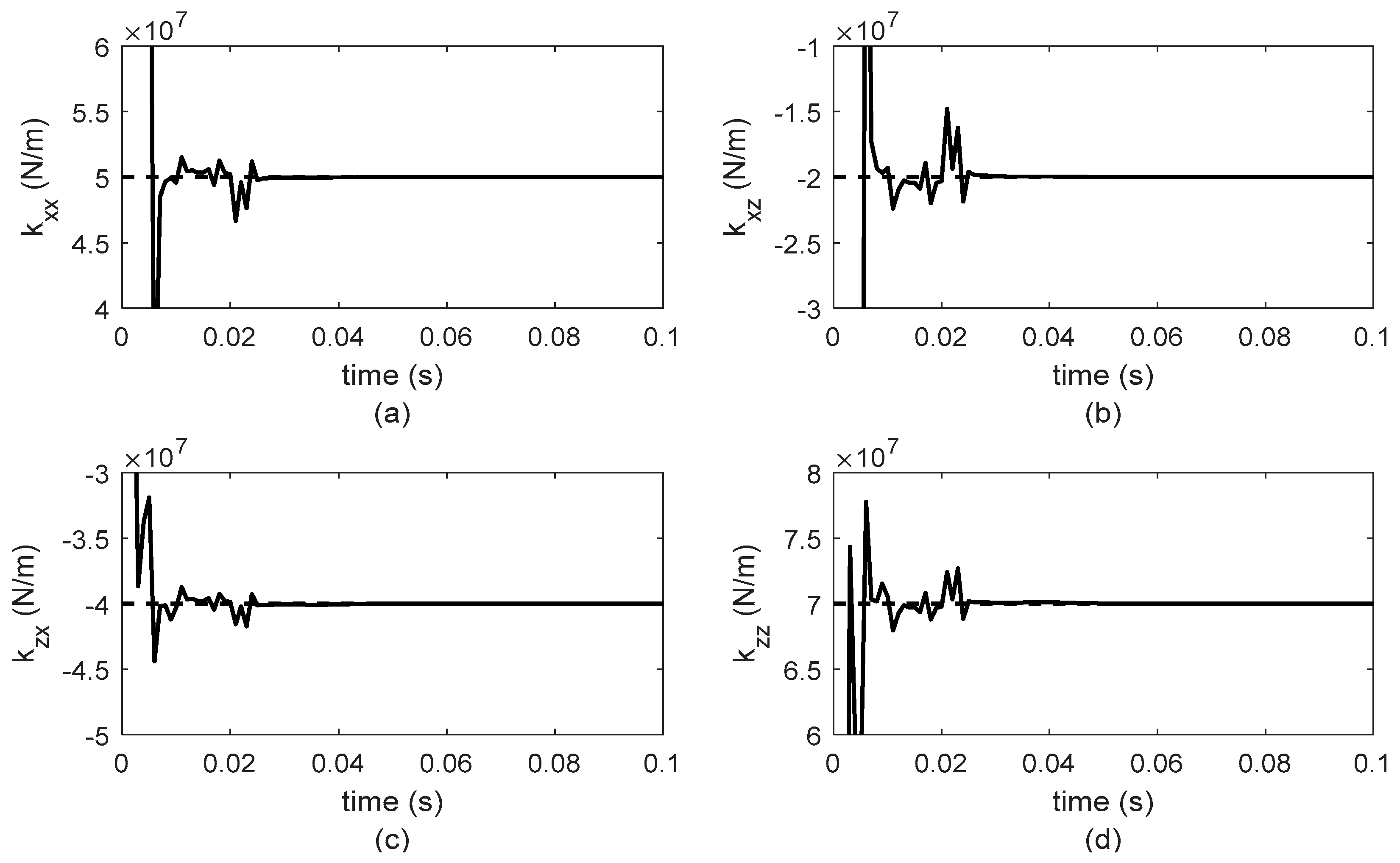
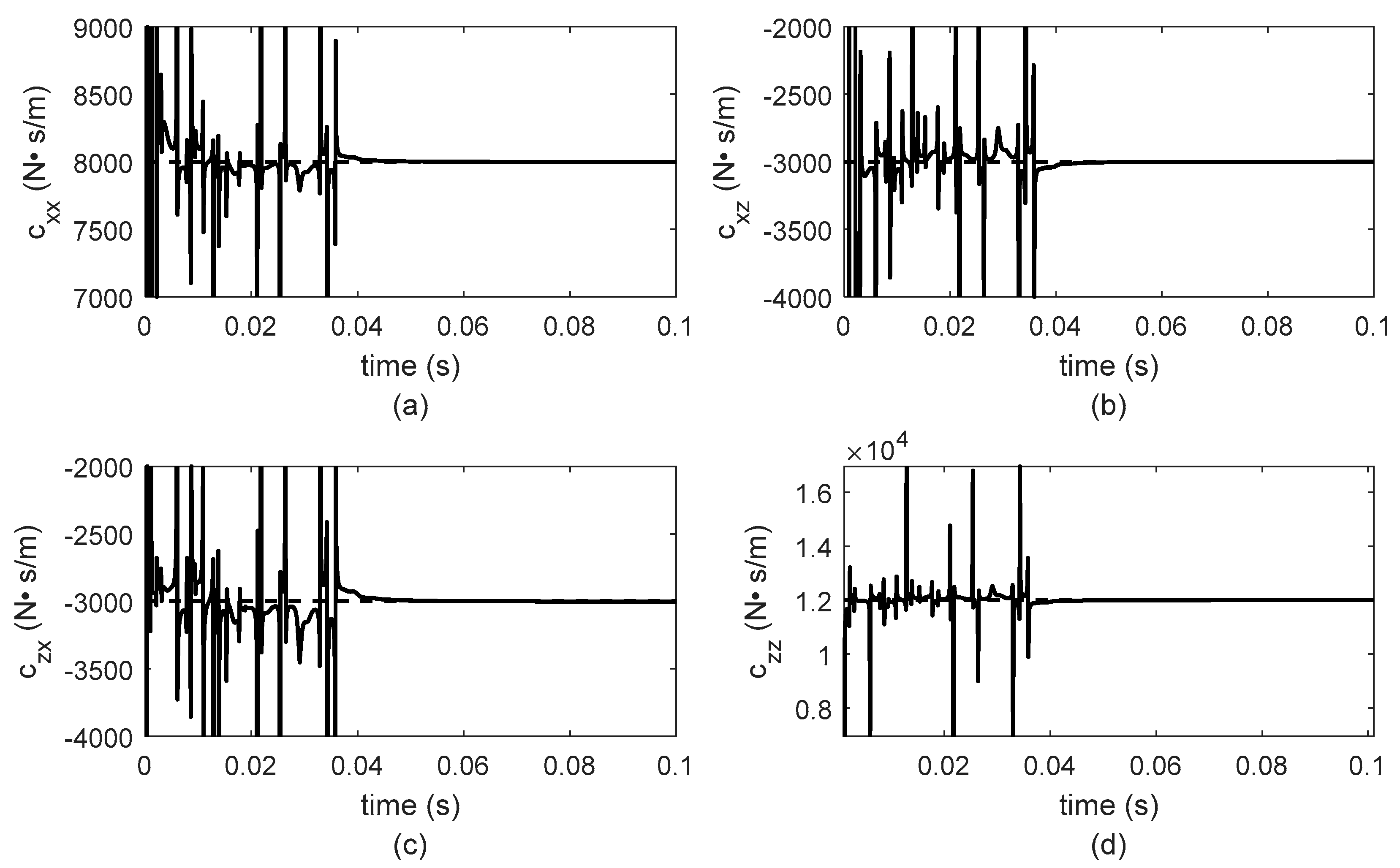
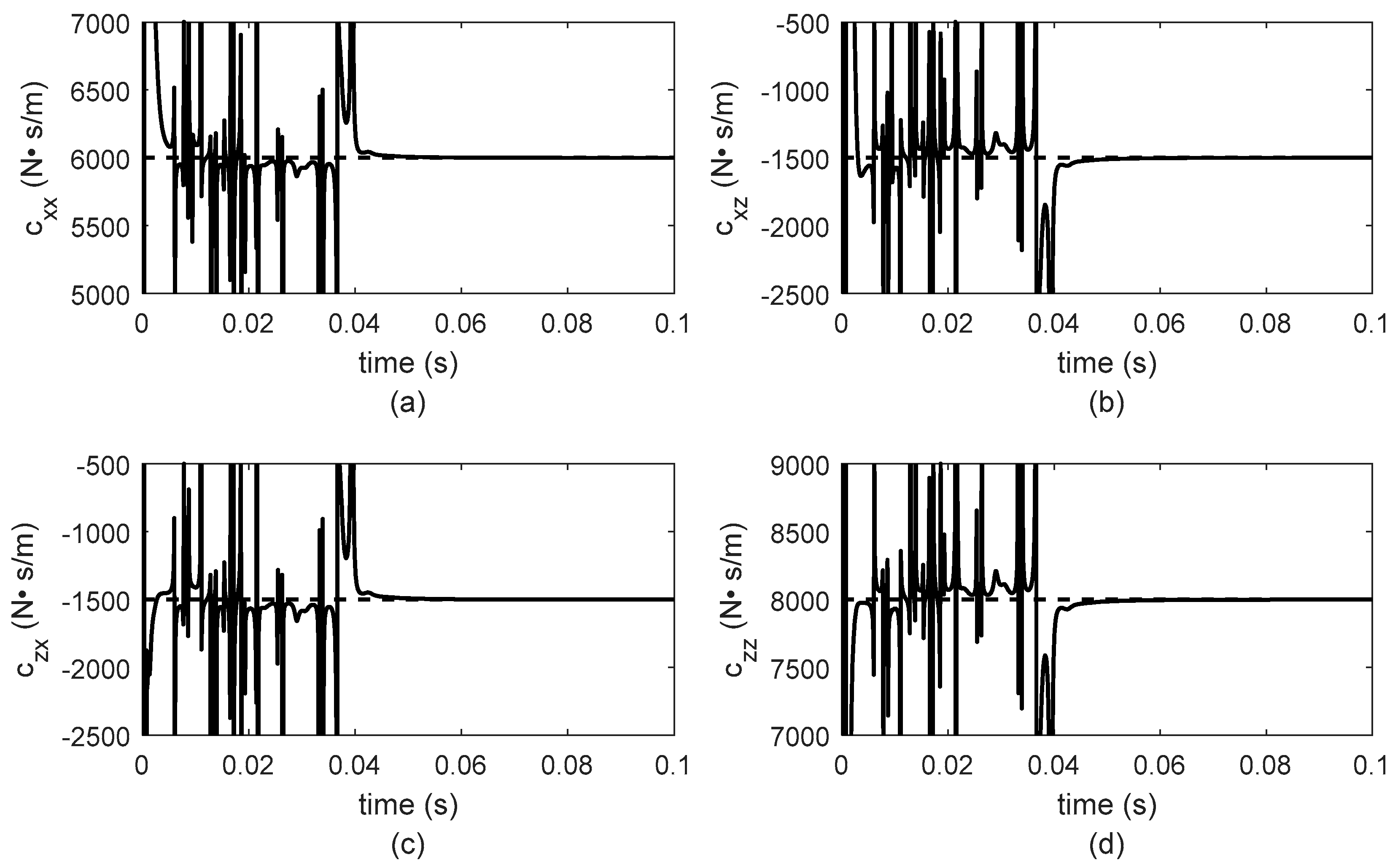
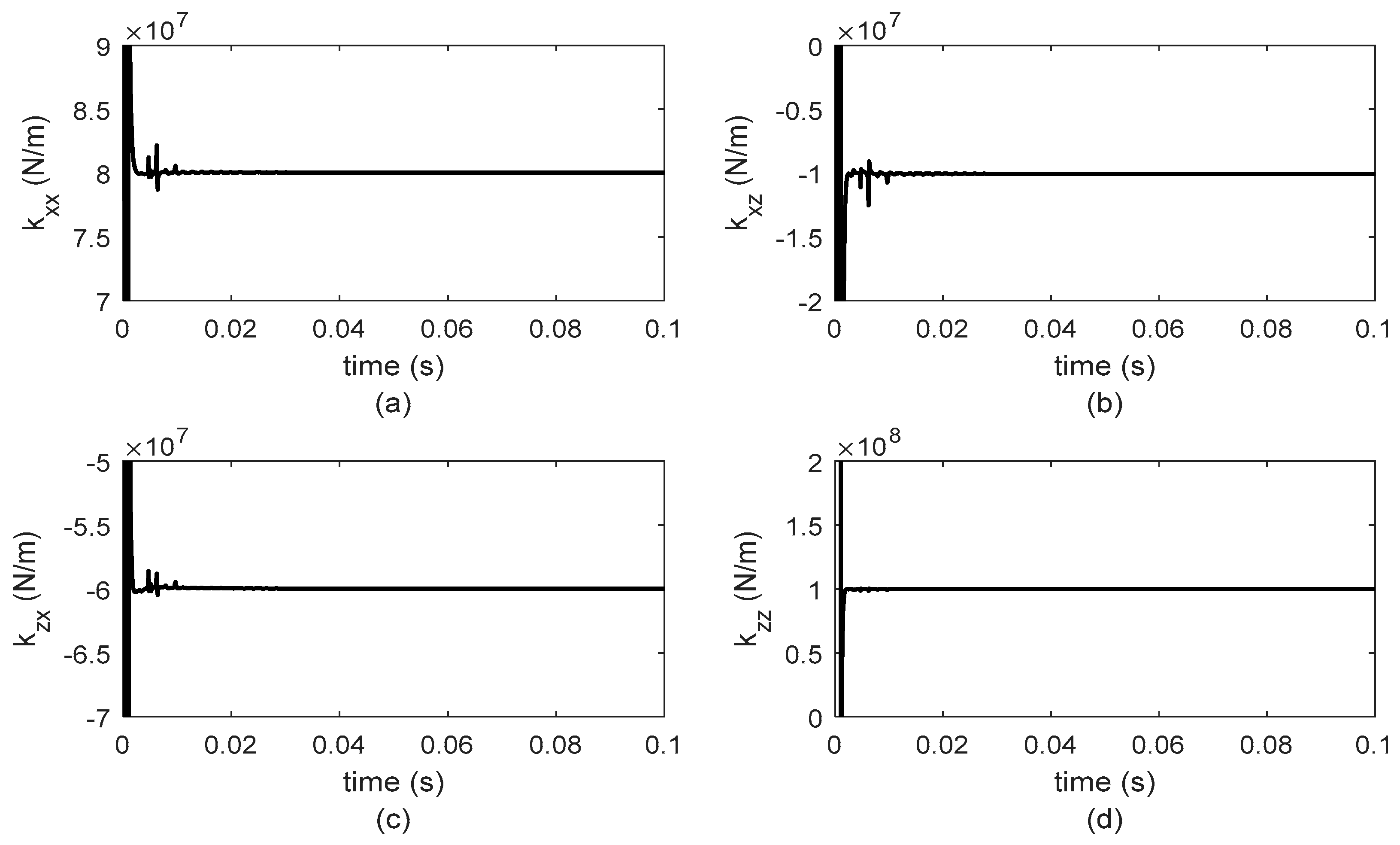
3.1. Algebraic Parameter Identification with Constant System Velocity

The displacement vector used in the algebraic identification procedure was obtained from Equation (7) by using the Newmark method for numerical integration and taking into account a constant rotational velocity of the rotor-bearing system.

In Figure 4, vibration signals at node 4 (corresponding to bearing 1 location) of the rotor-bearing system of Figure 3 are presented. This response is obtained for an operation rotational velocity $\mathsf{\Omega }=600 \mathrm{rpm}$. These signals, the nodal slopes and the corresponding information of the nodes adjacent to the bearing locations are the required data to identify stiffness and damping parameters of the bearings.

Figure 5 and Figure 6 present the obtained results from the numerical simulation for the algebraic identification of stiffness and damping parameters for bearing 1, while Figure 7 and Figure 8 show the results corresponding to bearing 2. It is important to mention that the sample time used in the simulation was 0.1 milliseconds. However, by carrying out numerical simulations with different sample times, it was observed that the shorter the sampling period, the faster the identifier converges.

As can be observed in Figure 5, Figure 6, Figure 7 and Figure 8, the identification of both stiffness and damping parameters of the bearings is carried out in less than 0.1 s, and once the parameter reaches the identified value, this remains for the rest of the time period. For a better analysis of the identifier behavior, only results for 0.1 s are presented in Figure 5, Figure 6, Figure 7 and Figure 8, because it is important to observe the time that the identifier requires to converge to the estimated value.

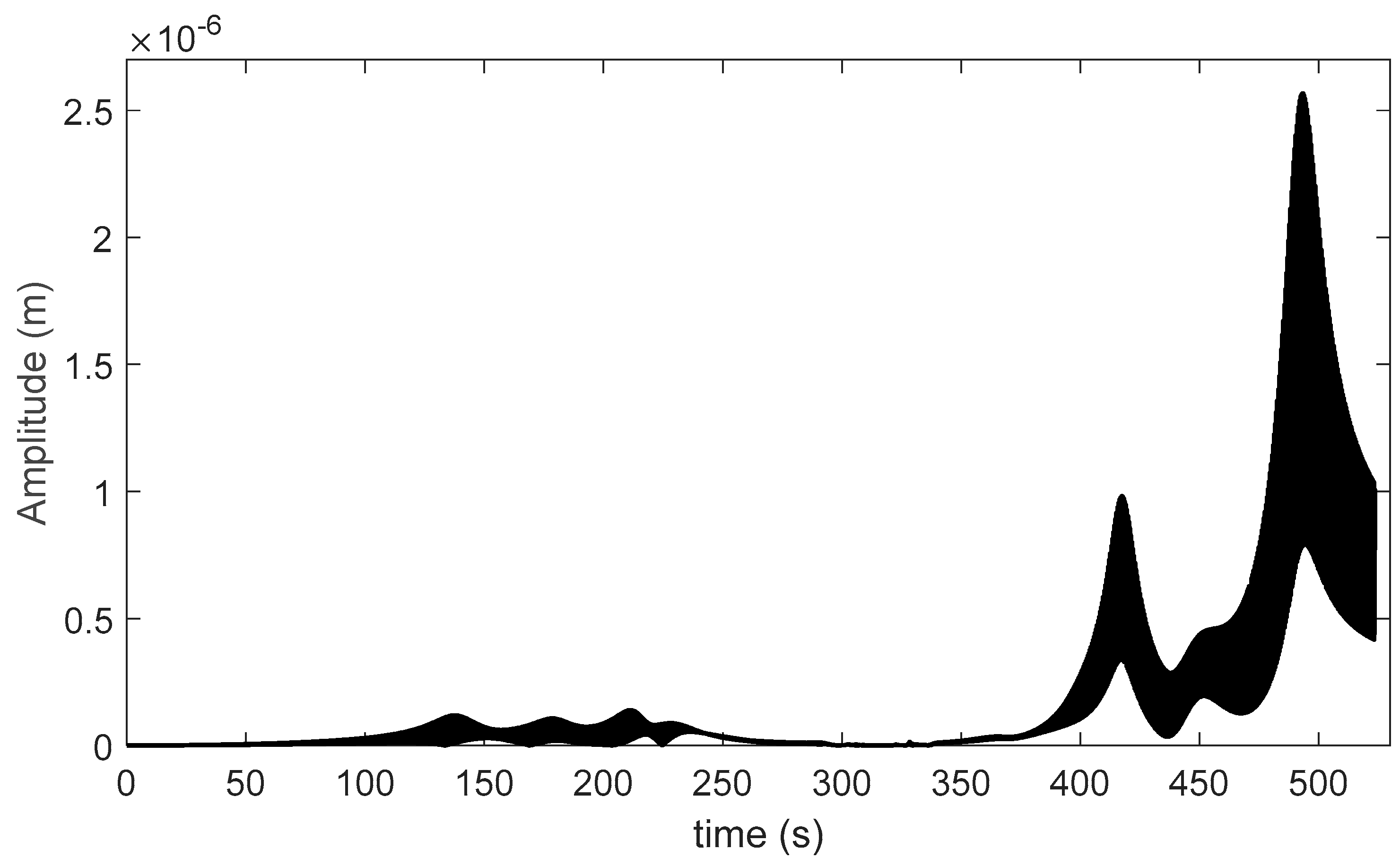
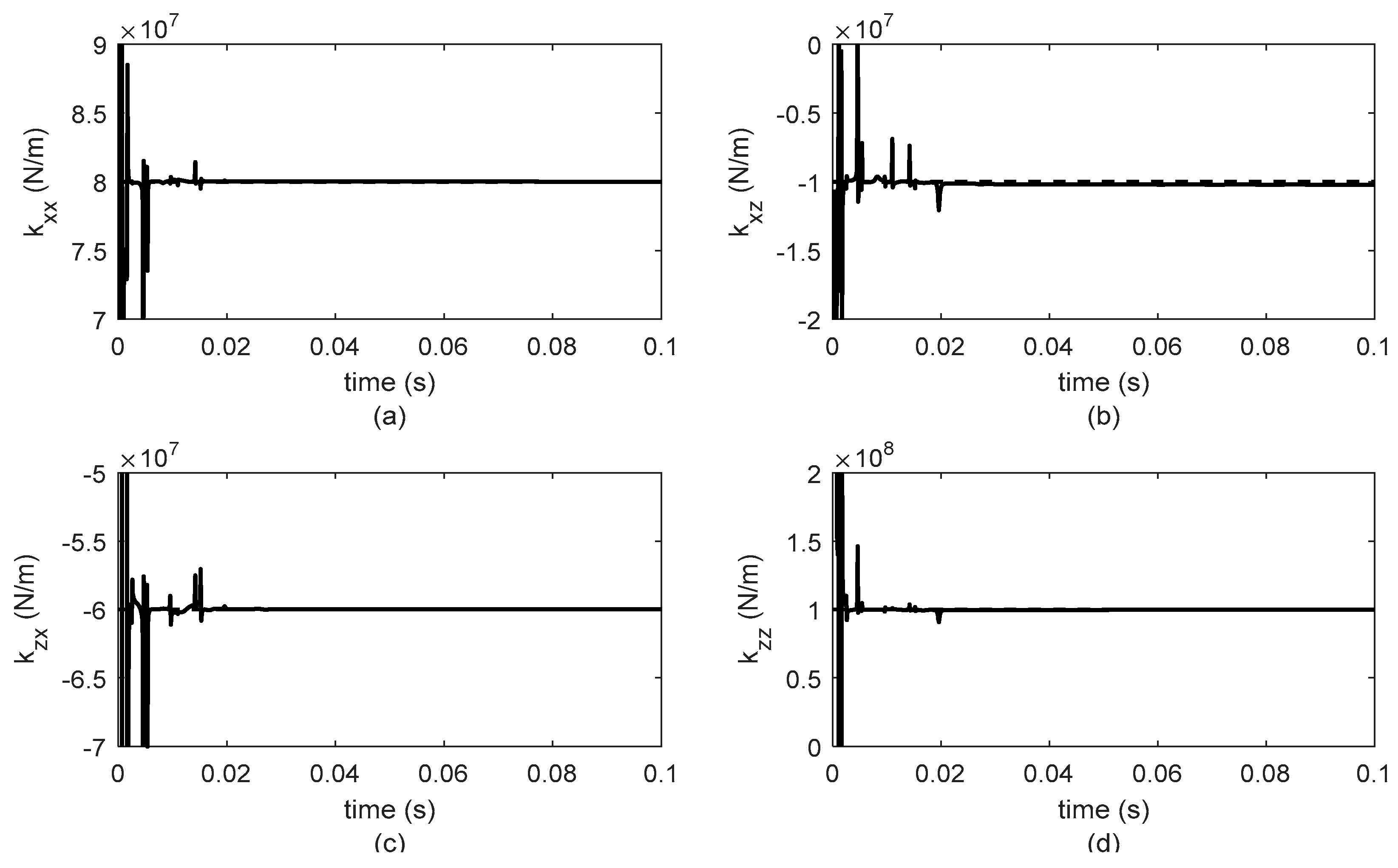
3.2. Algebraic Parameter Identification with Variable System Velocity

The displacement vector used as input data for the algebraic identification is obtained from Equation (3) by using the Newmark method for numerical integration and taking into account a linear ramp excitation with angular acceleration $\ddot{\varphi }=10 rad/s^2$. The rotor-bearing system response at node 4 is shown in Figure 9 where the vibratory behavior of the system in the location of bearing 1 can be appreciated.

In Figure 10, Figure 11, Figure 12 and Figure 13, the behavior of the algebraic identifier for bearing stiffness and damping parameters of both bearings (placed at nodes 4 and 8) is shown as a function of time.

As in the case of constant rotor system velocity, stiffness and damping bearing parameters are identified in les tan 0.1 s as can be observed in Figure 10, Figure 11, Figure 12 and Figure 13. Furthermore, the parameter values remain constant until the rotor-bearing system reaches its nominal operation velocity. For a better analysis of the identifier behavior, the results for 0.1 s are presented in Figure 10, Figure 11, Figure 12 and Figure 13 because it is important to observe the required time for the identifier convergence. The sample time used to solve Equation (3) using the Newmark method was 0.1 milliseconds. The numerical solution of Equation (3) was used as input data for the proposed algebraic identifier. Moreover, achieving this sample time with diverse data acquisition systems for experimental implementation was verified.

4. Discussion

Different numerical simulations were carried out in order to determine the robustness of the proposed identifiers under different conditions for the rotor-bearing system velocity. For the constant velocity case, different magnitudes for the rotor system velocity were considered, while for the variable velocity case, different ramps of excitation were explored.

Figure 14 shows results for the algebraic identification of stiffness and damping parameters for bearing 1 at a constant operation velocity of the rotor-bearing system of 50,000 rpm. A rapid identifier convergence to the estimated values can be observed, meaning that an increase in operation velocity does not affect the identifier performance. It is important to mention that, while the results for the identification of damping parameters of bearing 1 and the stiffness and damping parameters of bearing 2 are not presented, these parameters are correctly identified in less than 0.1 s.

The identifier performance for different ramps’ excitation was analyzed. The acceleration values considered for numerical simulation were: $\ddot{\varphi }=10 rad/s^2$, $\ddot{\varphi }=100 rad/s^2$, $\ddot{\varphi }=1000 rad/s^2$, $\ddot{\varphi }=3000 rad/s^2$ and $\ddot{\varphi }=6000 rad/s^2$. The result for $\ddot{\varphi }=10 rad/s^2$ were reported in the previous section. Due to the similar behavior of the identifier with different acceleration values, only results for $\ddot{\varphi }=6000 rad/s^2$ are shown here. The rotor-bearing system response for a ramp of excitation with the mentioned value of acceleration at node 4 (bearing 1 location) is presented in Figure 15. It can be seen that there is a considerable change in the time scale in comparison with Figure 9 because the acceleration is increased 600 times.

The algebraic identification performance under the conditions described above is shown in Figure 16, Figure 17, Figure 18 and Figure 19 where the estimation for the stiffness and damping bearings parameter is visualized. For this simulation, the system response in Figure 15 is used as input data.

From the results presented in Figure 16, Figure 17, Figure 18 and Figure 19, it can be observed that despite the linear ramp excitation being 600 times faster than the corresponding one in Figure 9, the proposed identifier rapidly converges to the estimated values and remains in these values for the rest of the time period. Note that the algebraic identifier is not affected by the system’s acceleration and only depends on the displacement vector at each instance. The robustness of the algebraic identification method against acceleration ramp variations had already been proved by Mendoza-Larios et al. [36] but only for the identification of unbalance parameters in rotor-bearing parameters.

Furthermore, the obtained results for both cases, constant and variable rotor-bearing velocity, show a transient state of the identifiers before the convergence to the estimated values of stiffness and damping bearing parameters. This behavior is due to the sample time used in the numerical simulations of the identifiers for solving the iterated integrals of Equations (15) and (24), which utilize the trapezoidal rule. According to Kharab and Guenther [41], this method presents major calculation errors in comparison with other integration methods. However, it was found that the smaller the sample time the shorter the error in the trapezoidal rule calculation.

5. Conclusions

In this article the identification problem for stiffness and damping parameters of the supports in rotor-bearing systems was addressed. The system model was obtained by the finite element method and using a finite element type beam, which consider the effects of rotational inertia, gyroscopic moments and shear deformations. The algebraic identification technique was applied to the finite element model to obtain two identifiers for the stiffness and damping parameters attributable to the bearings. The first identifier considers a rotor-bearing system operating at a constant velocity, and the second with a linear ramp of excitation as a system velocity input. The numerical results present the identifier behavior showing a fast convergence and robustness in both operation conditions with different values of constant rotational velocity and ramp of acceleration. The numerical results indicate a fast convergence in the stiffness and damping parameters identification in less than 0.06 s for both considered operation conditions. It is important to mention that the convergence time of the identifier depends mainly on the sample time used in numerical simulations. An important characteristic of the proposed algebraic identifiers is that the unbalance parameters (magnitude and phase) are not needed for their development and implementation because only the vibratory response of the system at the bearings’ location and the adjacent nodes is required. As a first approach we have proved the proposed identifiers in rotor-bearing system models with constant rotordynamic coefficients. However, as a future work, the proposed identifiers can be used to numerically and experimentally determine rotordynamic coefficients, which are a function of the system rotational velocity as in the case of pressurized bearings, by adapting the identifier method to estimate non-constant functions. This is possible because in the mathematical model used for the identifiers’ development, only the effects (stiffness and damping) of the supports are considered without taking into account the nature of the bearings.

References

1. Koutromanos, I. Fundamentals of Finite Element Analysis: Linear Finite Element Analysis, 1st ed.; John Wiley & Sons: New York, NY, USA, 2018. [Google Scholar]
2. Mendoza-Larios, J.G.; Barredo, E.; Colín, J.; Blanco-Ortega, A.; Arias-Montiel, M.; Mayén, J. Computational platform for the analysis and simulation of rotor-bearing systems of multiple degrees of freedom. Rev. Int. Metod. Numer. 2020, 36, 1–10. [Google Scholar]
3. Shen, Z.; Chouvion, B.; Thouverez, F.; Beley, A. Enhanced 3D solid finite element formulation for rotor dynamics simulation. Finite Elem. Anal. Des. 2021, 195, 103584. [Google Scholar] [CrossRef]
4. Tiwari, R. Rotor System: Analysis and Identification, 1st ed.; CRC Press: Boca Raton, FL, USA, 2018. [Google Scholar]
5. Matsushita, O.; Tanaka, M.; Kobayashi, M.; Keogh, P.; Kanki, H. Vibrations of Rotating Machinery. Volume 2. Advanced Rotordynamics: Applications of Analysis, Troubleshooting and Diagnosis, 1st ed.; Springer Japan KK: Tokyo, Japan, 2019. [Google Scholar]
6. Breńkacz, L. Bearing Dynamic Coefficients in Rotordynamics. Computation Methods and Practical Applications, 1st ed.; Wiley-ASME: New York, NY, USA, 2021. [Google Scholar]
7. Narendiranath Babu, T.; Manvel Raj, T.; Lakshmanan, T. A review on application of dynamic parameters of journal bearing for vibration and condition monitoring. J. Mech. 2015, 31, 391–416. [Google Scholar] [CrossRef]
8. Tiwari, R.; Chougale, A. Identification of bearing dynamic parameters and unbalance state in a flexible rotor system fully levitated on active magnetic bearings. Mechatronics 2014, 24, 274–286. [Google Scholar] [CrossRef]
9. Xu, Y.; Zhou, J.; Jin, C.; Guo, Q. Identification of the dynamic parameters of active magnetic bearings based on the transfer matrix model updating method. J. Mech. Sci. Technol. 2016, 30, 2971–2979. [Google Scholar] [CrossRef]
10. Mao, W.; Han, X.; Liu, G.; Liu, J. Bearing dynamic parameters identification of a flexible rotor-bearing system based on transfer matrix method. Inverse Probl. Sci. Eng. 2016, 24, 372–392. [Google Scholar] [CrossRef]
11. Yao, J.; Liu, L.; Yang, F.; Scarpa, F.; Gao, J. Identification and optimization of unbalance parameters in rotor-bearing systems. J. Sound Vib. 2018, 431, 54–69. [Google Scholar] [CrossRef] [Green Version]
12. Colín-Ocampo, J.; Guitérrez-Wing, E.S.; Ramírez-Moroyoqui, F.J.; Abúndez-Pliego, A.; Blanco-Ortega, A.; Mayén, J. A novel methodology for the angular position identification of the unbalance force on asymmetric rotors by response polar plot analysis. Mech. Syst. Signal Process. 2017, 95, 172–186. [Google Scholar] [CrossRef]
13. Mao, W.; Li, J.; Huang, Z.; Liu, J. Bearing dynamic parameters identification for sliding bearing-rotor system with uncertainty. Inverse Probl. Sci. Eng. 2018, 26, 1094–1108. [Google Scholar] [CrossRef]
14. Chen, C.; Jing, J.; Cong, J.; Dai, Z. Identification of dynamic coefficients in circular journals bearings from unbalance response and complementary equations. Proc. Inst. Mech. Eng. Part J. Eng. Tribol. 2019, 233, 1016–1028. [Google Scholar] [CrossRef]
15. Rajasekhara, R.M.; Srinivas, J. An optimized bearing parameter identification approach from vibration response spectra. J. Vibroeng. 2019, 21, 1519–1532. [Google Scholar]
16. Wang, A.; Yao, W.; He, K.; Meng, G.; Cheng, X.; Yang, J. Analytical modelling and numerical experiment for simultaneous identification of unbalance and rolling-bearing coefficients of the continuous single-disc and single-span rotor-bearing system with Rayleigh beam model. Mech. Syst. Signal Process. 2019, 116, 322–346. [Google Scholar] [CrossRef]
17. Wang, X.; Li, H.; Meng, G. Rotordynamic coefficients of a controllable magnetorheological fluid lubricated floating ring bearing. Tribol. Int. 2017, 114, 1–14. [Google Scholar] [CrossRef]
18. Kang, Y.; Shi, Z.; Zhang, H.; Zhen, D.; Gu, F. A novel method for the dynamic coefficients identification of journal bearings using Kalman filter. Sensors 2020, 20, 565. [Google Scholar] [CrossRef] [PubMed] [Green Version]
19. Chen, Y.; Yang, R.; Sugita, N.; Mao, J.; Shinshi, T. Identification of bearing dynamic parameters and unbalanced forces in a flexible rotor system supported by oil-film bearings and active magnetic devices. Actuators 2021, 10, 216. [Google Scholar] [CrossRef]
20. Taherkhani, Z.; Ahmadian, H. Stochastic model updating of rotor support parameters using Bayesian approach. Mech. Syst. Signal Process. 2021, 158, 107702. [Google Scholar] [CrossRef]
21. Brito, G.C., Jr.; Machado, R.D.; Neto, A.C.; Kimura, L.Y. A method for the experimental estimation of direct and cross-coupled dynamic coefficients of tilting-pad journal bearings of vertical hydro-generators. Struct. Health Monit. 2021, 1–17. [Google Scholar] [CrossRef]
22. San Andrés, L.; Jeung, S.H. Orbit-model force coefficients for fluid film bearings: A step beyond linearization. ASME J. Eng. Gas Turbines Power 2015, 132, 022502. [Google Scholar]
23. Yang, L.H.; Wang, W.M.; Zhao, S.Q.; Sun, Y.H.; Yu, L. A new nonlinear dynamic analysis method of rotor system supported by oil-film journal bearings. Appl. Math. Model. 2014, 38, 5239–5255. [Google Scholar] [CrossRef]
24. Dyk, S.; Smolík, L.; Rendl, J. Predictive capability of various linearization approaches for floating-ring bearings in nonlinear dynamics of turbochargers. Mech. Mach. Theory 2020, 149, 103843. [Google Scholar] [CrossRef]
25. Nelles, O. Nonlinear System Identification. From Classical Approaches to Neural Networks, Fuzzy Models, and Gaussian Processes, 1st ed.; Springer Nature: Cham, Switzerland, 2020. [Google Scholar]
26. Tangirala, A.K. Principles of System Identification: Theory and Practice, 1st ed.; CRC Press: Boca Raton, FL, USA, 2015. [Google Scholar]
27. Aster, R.C.; Borchers, B.; Thurber, C.H. Parameter Estimation and Inverse Problems, 3rd ed.; Elsevier: Cambridge, MA, USA, 2019. [Google Scholar]
28. Arias-Montiel, M.; Beltrán-Carbajal, F.; Silva-Navarro, G. On-line algebraic identification of eccentricity parameters in active rotor-bearing systems. Int. J. Mech. Sci. 2014, 85, 152–159. [Google Scholar] [CrossRef]
29. Sira-Ramírez, H.; García-Rodríguez, C.; Cortés-Romero, J.; Luviano-Juárez, A. Algebraic Identification and Estimation Methods in Feedback Control Systems, 1st ed.; John Wiley & Sons: West Sussex, UK, 2014. [Google Scholar]
30. Trujillo-Franco, L.G.; Abundis-Fong, H.F.; Campos-Amezcua, R.; Gomez-Martinez, R.; Martinez-Perez, A.I.; Campos-Amezcua, A. Single output and algebraic modal parameters identification of a wind turbine blade: Experimental results. Appl. Sci. 2021, 11, 3016. [Google Scholar] [CrossRef]
31. Silva-Navarro, G.; Beltrán-Carbajal, F.; Trujillo-Franco, L.G.; Peza-Solís, J.F.; García-Pérez, O.A. Online estimation techniques for natural and excitation frequencies on MDOF vibrating mechanical systems. Actuators 2021, 10, 41. [Google Scholar] [CrossRef]
32. Trujillo-Franco, L.G.; Silva-Navarro, G.; Beltrán-Carbajal, F.; Campos-Mercado, E.; Abundis-Fong, H.F. On-line modal parameter identification applied to linear and nonlinear vibration absorbers. Actuators 2020, 9, 119. [Google Scholar] [CrossRef]
33. Beltrán-Carbajal, F.; Silva-Navarro, G. Generalized nonlinear stiffness identification on controlled mechanical vibrating systems. Asian J. Control 2019, 21, 1281–1292. [Google Scholar] [CrossRef]
34. Beltran-Carbajal, F.; Silva-Navarro, G.; Trujillo-Franco, L.G. On-line parametric estimation of damped multiple frequency oscillations. Electr. Power Syst. Res. 2018, 154, 423–432. [Google Scholar] [CrossRef]
35. Beltrán-Carbajal, F.; Silva-Navarro, G.; Trujillo-Franco, L.G. A sequential algebraic parametric identification approach for nonlinear vibrating mechanical systems. Asian J. Control 2017, 19, 1–11. [Google Scholar] [CrossRef]
36. Mendoza-Larios, J.G.; Colín-Ocampo, J.; Blanco-Ortega, A.; Abúndez-Pliego, A.; Gutiérrez-Wing, E.S. Automatic balancing of a rotor-bearing system: On-line algebraic identifier for a rotordynamic balancing system. Rev. Ibearoam. Autom. Inform. Ind. 2016, 13, 281–292. [Google Scholar]
37. Colín-Ocampo, J.; Mendoza-Larios, J.G.; Blanco-Ortega, A.; Abúndez-Pliego, A.; Gutiérrez-Wing, E.S. Unbalance determination in rotor-bearing systems at constant velocity: Algebraic identification method. Ing. Mec. Tecnol. Des. 2016, 5, 385–394. (In Spanish) [Google Scholar]
38. Beltrán-Carbajal, F.; Silva-Navarro, G. On the algebraic parameter identification of vibrating mechanical systems. Int. J. Mech. Sci. 2015, 92, 178–186. [Google Scholar] [CrossRef]
39. Beltrán-Carbajal, F.; Silva-Navarro, G.; Arias-Montiel, M. Active unbalance control of rotor systems using on-line algebraic identification methods. Asian J. Control 2013, 15, 1627–1637. [Google Scholar] [CrossRef]
40. Lalanne, M.; Ferraris, G. Rotordynamics Prediction in Engineering, 2nd ed.; John Wiley & Sons: West Sussex, UK, 1998. [Google Scholar]
41. Kharab, A.; Guenther, R.B. An Introduction to Numerical Methods. A MATLAB Approach; CRC Pess: Boca Raton, FL, USA, 2019. [Google Scholar]
Figure 1. Beam-like finite element for the modelling of the rotor-bearing shaft.
Mathematics 09 02747 g001
Figure 2. Stiffness and damping parameters in bearings [40].
Mathematics 09 02747 g002
Figure 3. Rotor-bearing system scheme [40].
Mathematics 09 02747 g003
Figure 4. Vibration signal at node 4 (bearing 1) at 600 rpm: (a) X direction; (b) Z direction.
Mathematics 09 02747 g004
Figure 5. Identified stiffness parameters for bearing 1 at 600 rpm. (a) k x x , (b) k x z , (c) k z x , (d) k z z .
Mathematics 09 02747 g005
Figure 6. Identified damping parameters for bearing 1 at 600 rpm. (a) c x x , (b) c x z , (c) c z x , (d) c z z .
Mathematics 09 02747 g006
Figure 7. Identified stiffness parameters for bearing 2 at 600 rpm. (a) k x x , (b) k x z , (c) k z x , (d) k z z .
Mathematics 09 02747 g007
Figure 8. Identified damping parameters for bearing 2 at 600 rpm. (a) c x x , (b) c x z , (c) c z x , (d) c z z .
Mathematics 09 02747 g008
Figure 9. System vibratory response at node 4 with a linear ramp of excitation of 10   r a d / s 2 .
Mathematics 09 02747 g009
Figure 10. Identified stiffness parameters for bearing 1 with a linear ramp of excitation of 10   r a d / s 2 . (a) k x x , (b) k x z , (c) k z x , (d) k z z .
Mathematics 09 02747 g010
Figure 11. Identified damping parameters for bearing 1 with a linear ramp of excitation of 10   r a d / s 2 . (a) c x x , (b) c x z , (c) c z x , (d) c z z .
Mathematics 09 02747 g011
Figure 12. Identified stiffness parameters for bearing 2 with a linear ramp of excitation of 10   r a d / s 2 . (a) k x x , (b) k x z , (c) k z x , (d) k z z .
Mathematics 09 02747 g012
Figure 13. Identified damping parameters for bearing 2 with a linear ramp of excitation of 10   r a d / s 2 . (a) c x x , (b) c x z , (c) c z x , (d) c z z .
Mathematics 09 02747 g013
Figure 14. Identified stiffness parameters for bearing 1. (a) k x x , (b) k x z , (c) k z x , (d) k z z at 50,000 rpm.
Mathematics 09 02747 g014
Figure 15. System vibratory response at node 4 with a linear ramp excitation with acceleration of 6000   r a d / s 2 .
Mathematics 09 02747 g015
Figure 16. Identified stiffness parameters for bearing 1 with a ramp excitation of 6000   r a d / s 2 . (a) k x x , (b) k x z , (c) k z x , (d) k z z .
Mathematics 09 02747 g016
Figure 17. Identified damping parameters for bearing 1 with a ramp excitation of 6000   r a d / s 2 . (a) c x x , (b) c x z , (c) c z x , (d) c z z .
Mathematics 09 02747 g017
Figure 18. Identified stiffness parameters for bearing 2 with a ramp excitation of 6000   r a d / s 2 . (a) k x x , (b) k x z , (c) k z x , (d) k z z .
Mathematics 09 02747 g018
Figure 19. Identified damping parameters for bearing 2 with a ramp excitation of 6000   r a d / s 2 . (a) c x x , (b) c x z , (c) c z x , (d) c z z .
Mathematics 09 02747 g019