This section deals with the comparison of the above-described methods of numerical integration and Laplace inversion for several test problems.
5.1. Deterministic PDE Problem with Constant Coefficients
We start with simple one dimensional deterministic problem with a known analytical solution in order to check the viability of the proposed numerical integration techniques. The deterministic example corresponds to one fixed event
. Instead of the bounded spatial domain
, the whole real axis
is considered. Thus, no boundary conditions are needed. We also assume that
,
, and
are constants, i.e., the following wave equation is considered
subject to initial conditions
,
.
This problem admits an analytical solution that can be written in terms of Bessel function of the first kind, see [
23], p. 574, Equation 6.1.5, as follows
for
:
where
and
are the modified Bessel function of the first kind;
for
:
where
and
are Bessel function of the first kind.
In order to test the proposed numerical integration methods we apply Laplace transform, as described in
Section 2, and obtain a deterministic version of Equation (
13):
Applying the non-unitary Fourier transform with angular frequency
Equation (
13) takes the following form
Algebraic Equation (
30) is solved directly
Hence, the solution
of (
28) can be obtained by applying inverse Fourier transform to (
31).
In the next Example 1, we consider a particular case of Equation (
25) with constant coefficients and trigonometric initial conditions.
Example 1. Let us consider deterministic problem (25) with coefficients , , , and initial conditions and . Numerical solution is constructed in the truncated domain
,
,
, for discrete uniformly distributed nodes (
16),
,
, by applying the described in previous section methods, see Algorithm 1. We set
.
Applying the inverse Fourier transform to (
31), one obtains
where
is the imaginary unit. Once the solution of ODE (
28) is obtained, formula (
15) is used to restore the solution of the PDE while using various numerical integration techniques.
Note that Equation (
25) admits the analytical solution, as described above. Because the function
is close to zero, we compute the relative error of the discrete numerical solution at the mesh nodes in order to estimate the accuracy of the methods
where
is the matrix of numerical solution
,
,
, as computed by Algorithm 1;
is the reference value at the point
. In this example, as the exact solution is known, the reference value is equal to this exact solution. For other cases where the exact solution is not available, a reference value is obtained using accurate finite difference method (FDM) for solving the original PDE (
7). The total computational time for the proposed methods are presented in
Table 1, together with the maximum of
.
The adaptative quadrature (MatLAB function
integral [
24]) has the same order of accuracy as the midpoint rule, but it requires greater computational resources. Thus, it will not be considered in further more complicated examples.
For the Talbot algorithm
is chosen to guarantee the accuracy up to 10 significant digits [
22]. Even in that case, the method performs much faster than standard numerical integration methods for (
15). Thus, the Talbot inverse method is found to be the most effective method for the deterministic case with constant coefficients.
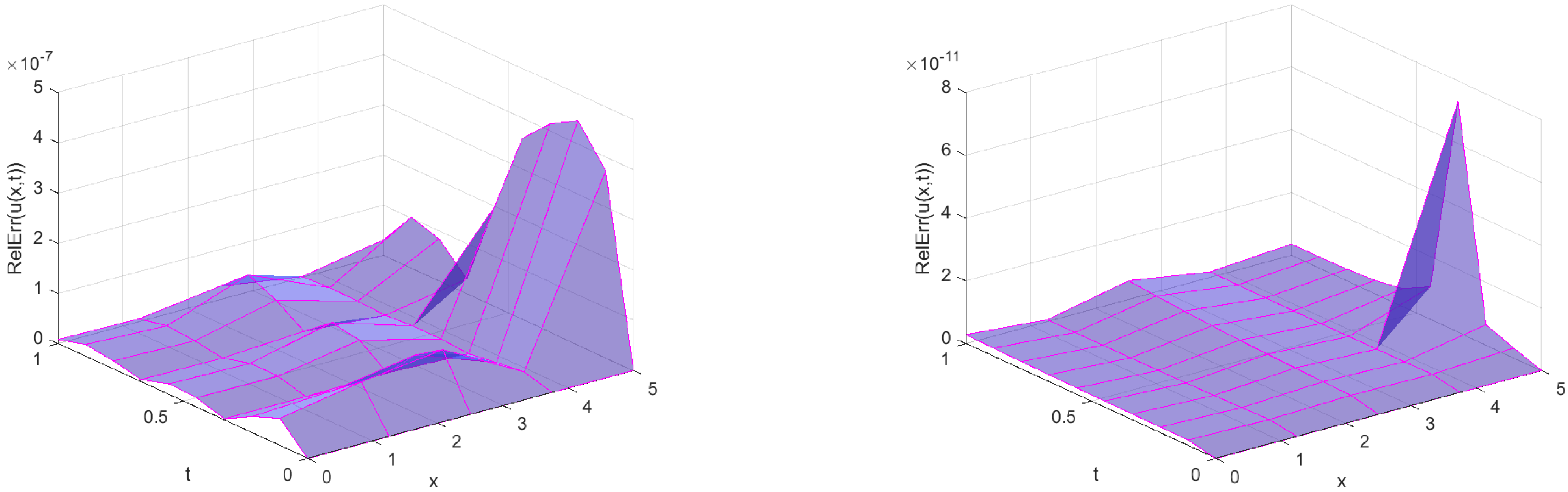
The relative errors for Midpoint rule and Talbot inverse methods are plotted in
Figure 1. Because no boundary conditions are posed for the problem, the largest values of the relative errors are situated at the boundary
.
Table 2 presents a comparison of GL and EF-GL quadratures in terms of the maximum relative error and the CPU-time varying the number of nodes
. It is important to notice that the CPU-time may vary from simulation to simulation, thus only the order should be taken into account. In the case of GL quadrature, we find out that the computational time is similar with increasing number of nodes, while the CPU-time for EF-GL method is increasing exponentially. The convergence of the GL quadrature is shown, while taking the results shown in
Table 1 into account: the error reduces significantly with an increasing number of nodes. The potential improvement of the GL method by the exponential fitting expectedly has higher computational cost, due to the solution of the nonlinear system at each point of the computational domain. However, the accuracy of the EF-Gl quadrature for this example with oscillating integrand has not been improved when comparing with the standard GL rule. Thus, it will not be considered in further more complicated examples.
The accuracy of the midpoint rule depends on the truncation
and step size
. A bigger domain, as well as smaller step size, lead to an increased computational time.
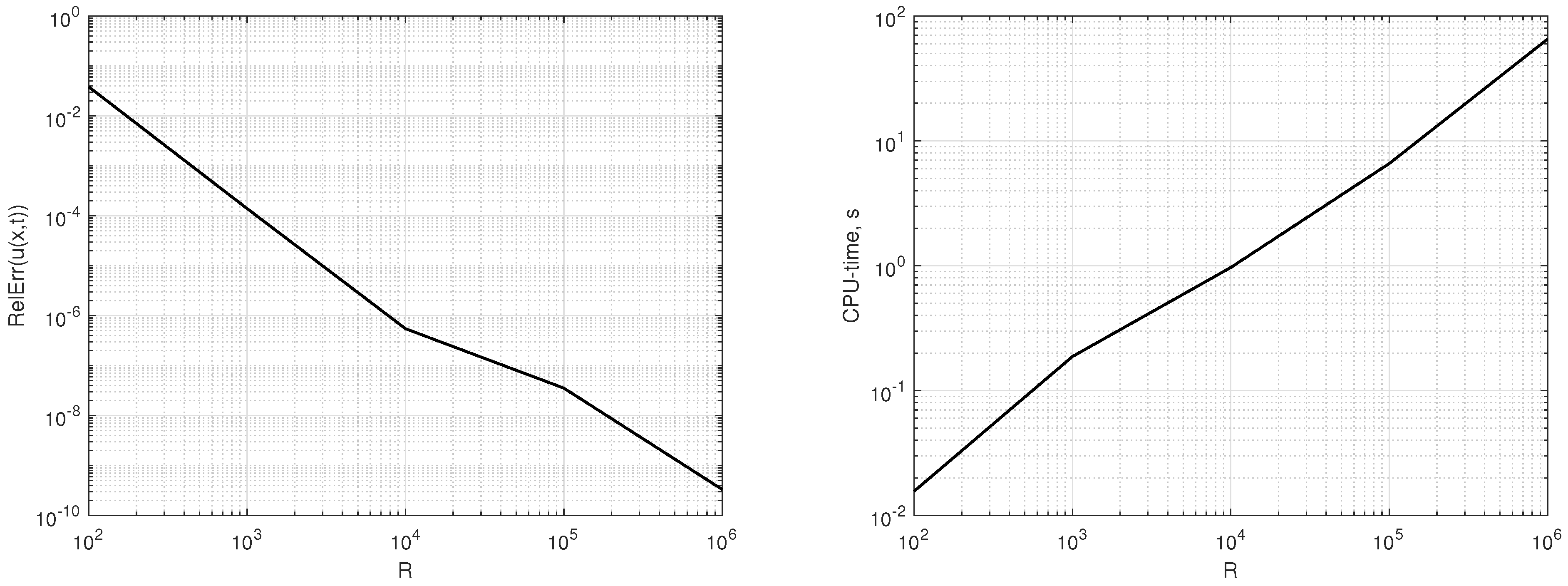
Figure 2 presents the plots of errors and the CPU-time for fixed step size
with respect to increasing domain. The accuracy in dependence on the step size
is also studied. In
Table 3, the maximum relative error is reported for various
and fixed
. The maximum relative error is decreasing with step size until
(
); further fragmentation of the step size does not reduce the error for
.
5.2. Deterministic PDE with Non-Constant Coefficients
In the case of non-constant coefficients in (
13), the analytical solution is not always available; thus, FDM is applied to construct a reference numerical solution. Note that the function
that is used in expression (
17) means the value of the numerical solution of the ODE (
13) at the fixed point
for fixed parameter
.
Equation (
13) is discretized by the central differences on the same mesh
,
, as follows
where
stands for the approximated value of
at the node
. The values at the boundaries are found from the boundary conditions by applying the Laplace transform
Hence, the integrand (
17) has to be evaluated at each fixed node of the computational grid in order to approximate integral (
15), which provokes a significant augment of the CPU-time. In the next example, we increase the complexity by regarding a variable coefficients deterministic problem.
Because the analytical solution for the deterministic PDE problem in general form (
7) is not available, a numerical method has to be employed to obtain the reference numerical solution. We consider an explicitly centred in time and space finite difference scheme for the mesh function
:
where
,
. The initial conditions (
8) are used in order to obtain the solution at the first time levels
and
. The derivative in (
8) is approximated by the forward difference. Because the considered scheme is conditionally stable, the step sizes
and
are chosen to guarantee the stability. In order to obtain a good approximation, which could be considered as the reference solution, the mesh should be chosen appropriately fine.
Example 2. Let us consider a deterministic vibrating string problem (7) on rectangle , , . We set non-constant coefficients , , , initial conditions and , and boundary conditions . The numerical solution is constructed by the Algorithm 1, choosing
,
. For the midpoint rule,
and
are used.
Table 4 presents the comparison of the methods in terms of maximum relative error and computational time. The reference solution is the numerical solution that is computed by the FDM (
36) in refined mesh (
,
= 16,000), which preserves the stability of the scheme. Because an explicit method is used and no iterative procedures are needed for solving nonlinear system at each time-level, the total computational time is comparably small: 0.15 s.
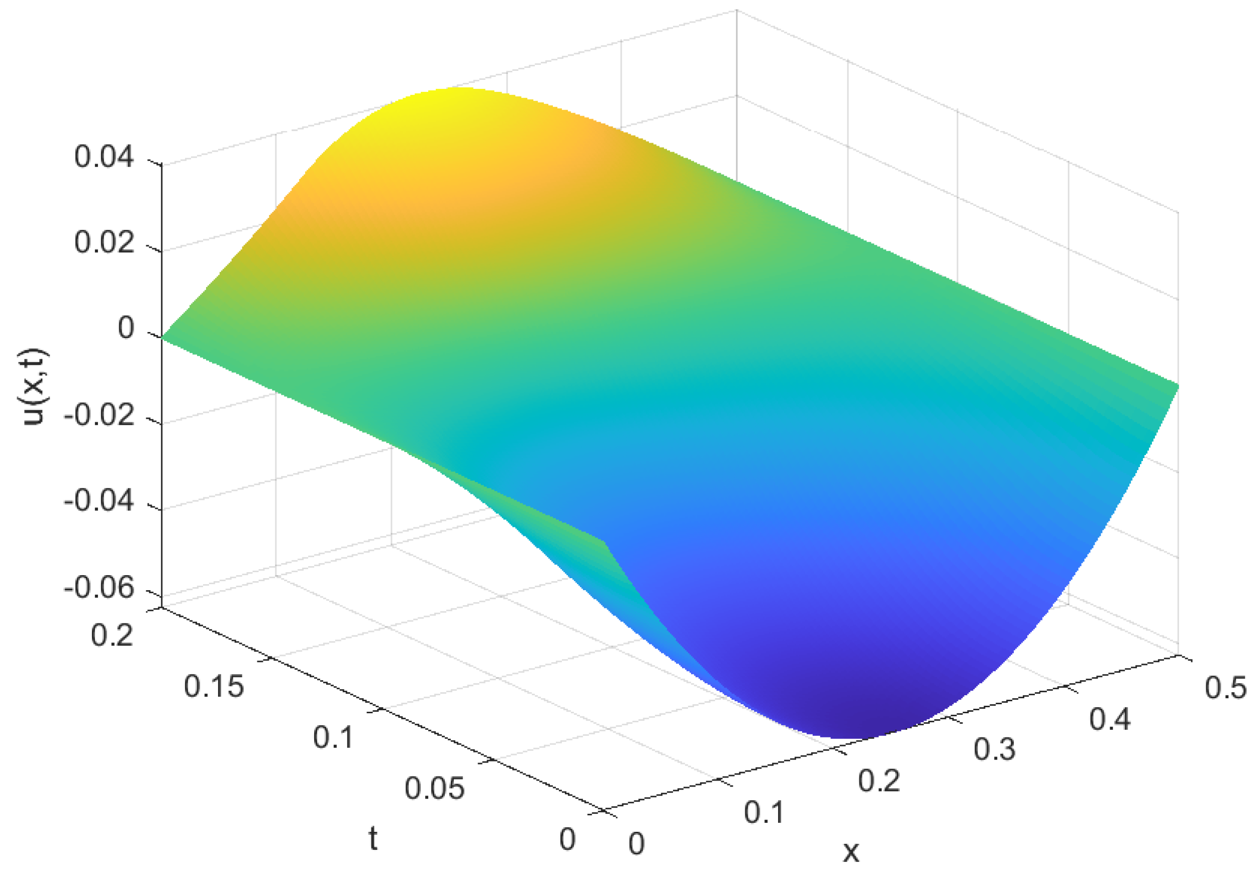
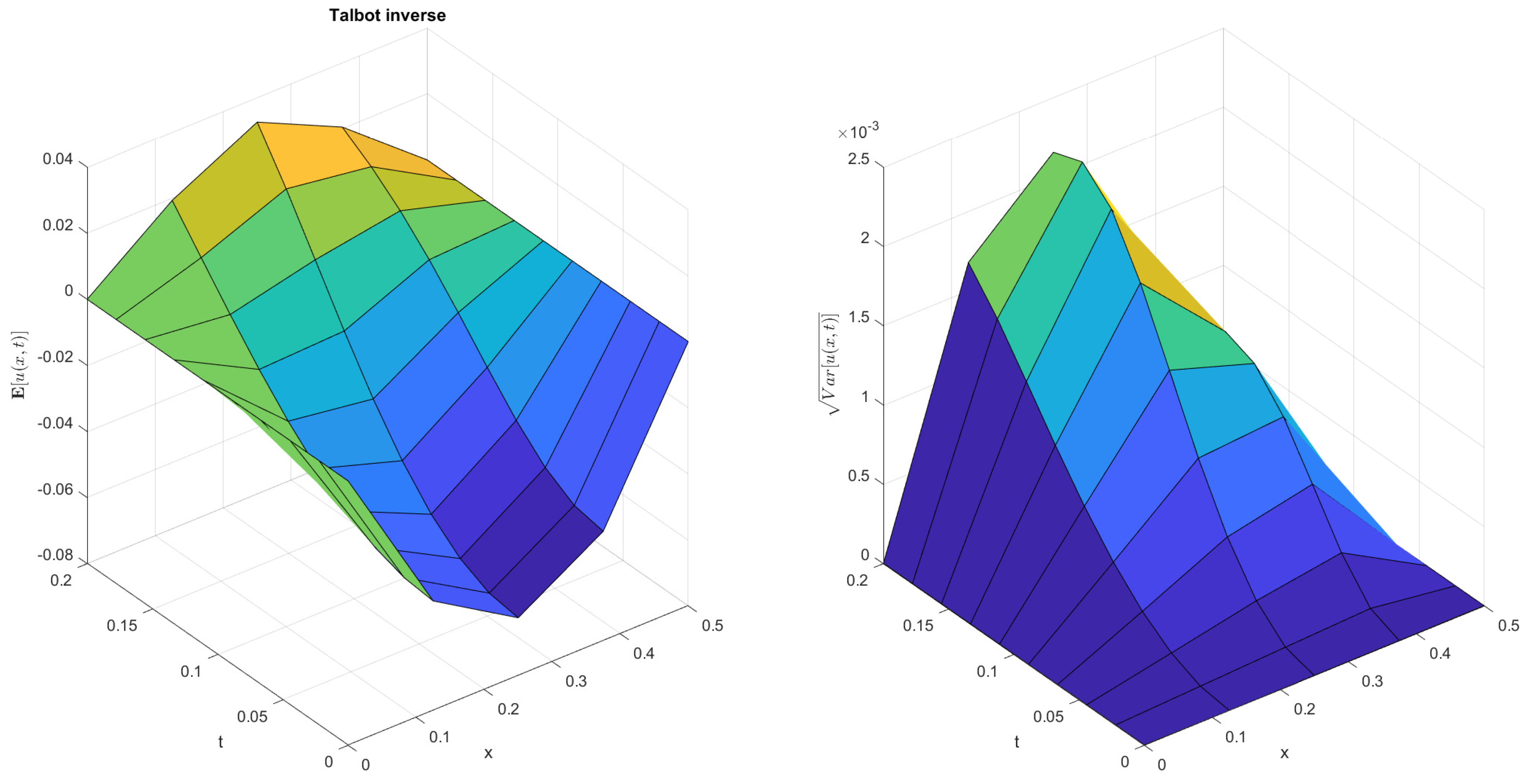
Figure 3 plots the reference solution.
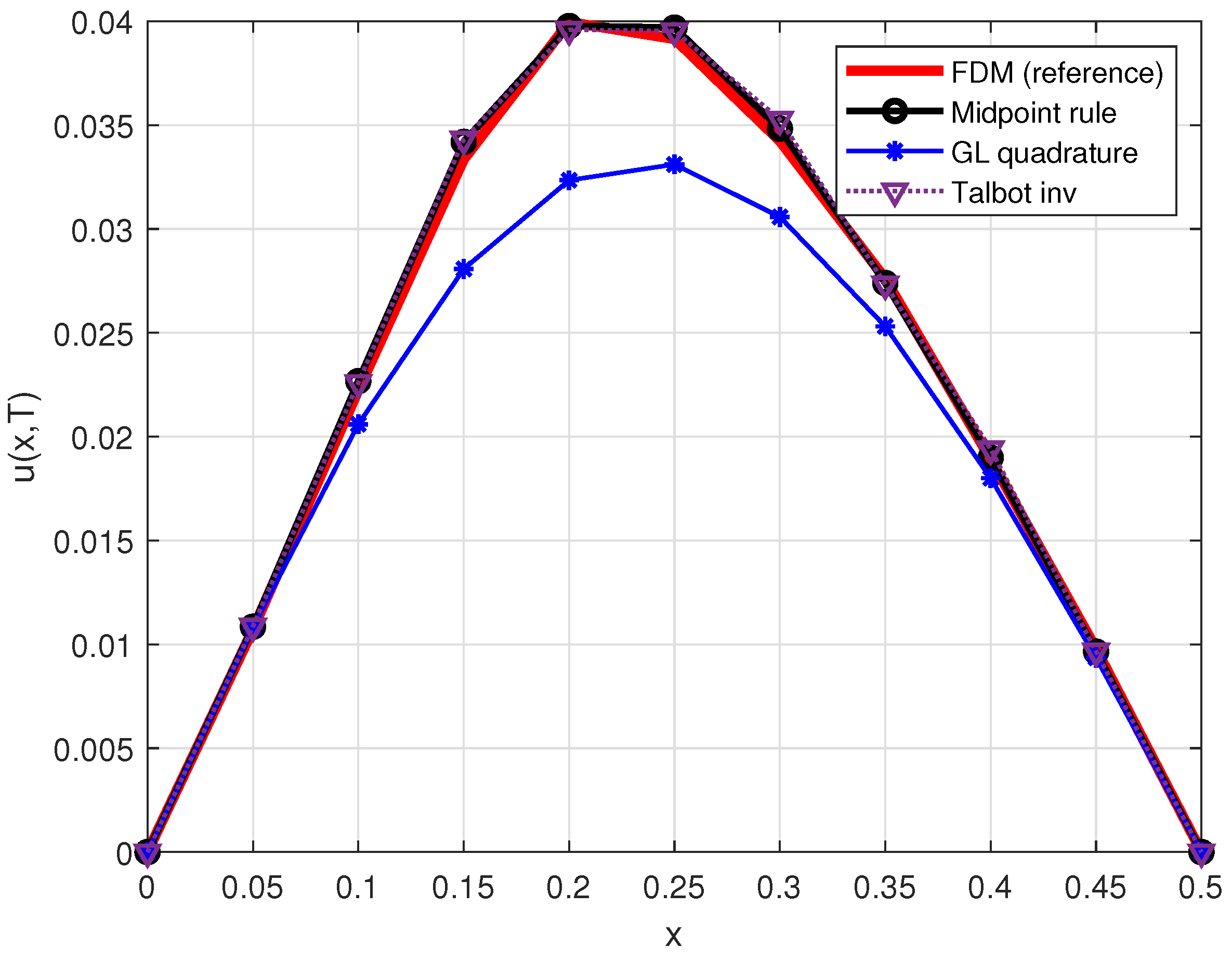
Figure 4 plots the solution at the moment
. The midpoint rule and Talbot inverse method perform more accurately than GL quadrature of nine nodes, but they require more computational time due to larger number of calls of integrand (
17). However, taking 25 nodes in the GL quadrature, the accuracy has been improved significantly.
5.3. Random PDE with Constant Coefficients
In this subsection, we deal with random models with constant coefficient random variables. It is remarkable that, in this case, we need not only the computation of the approximation s.p. solution, but also the computation of its statistical moments.
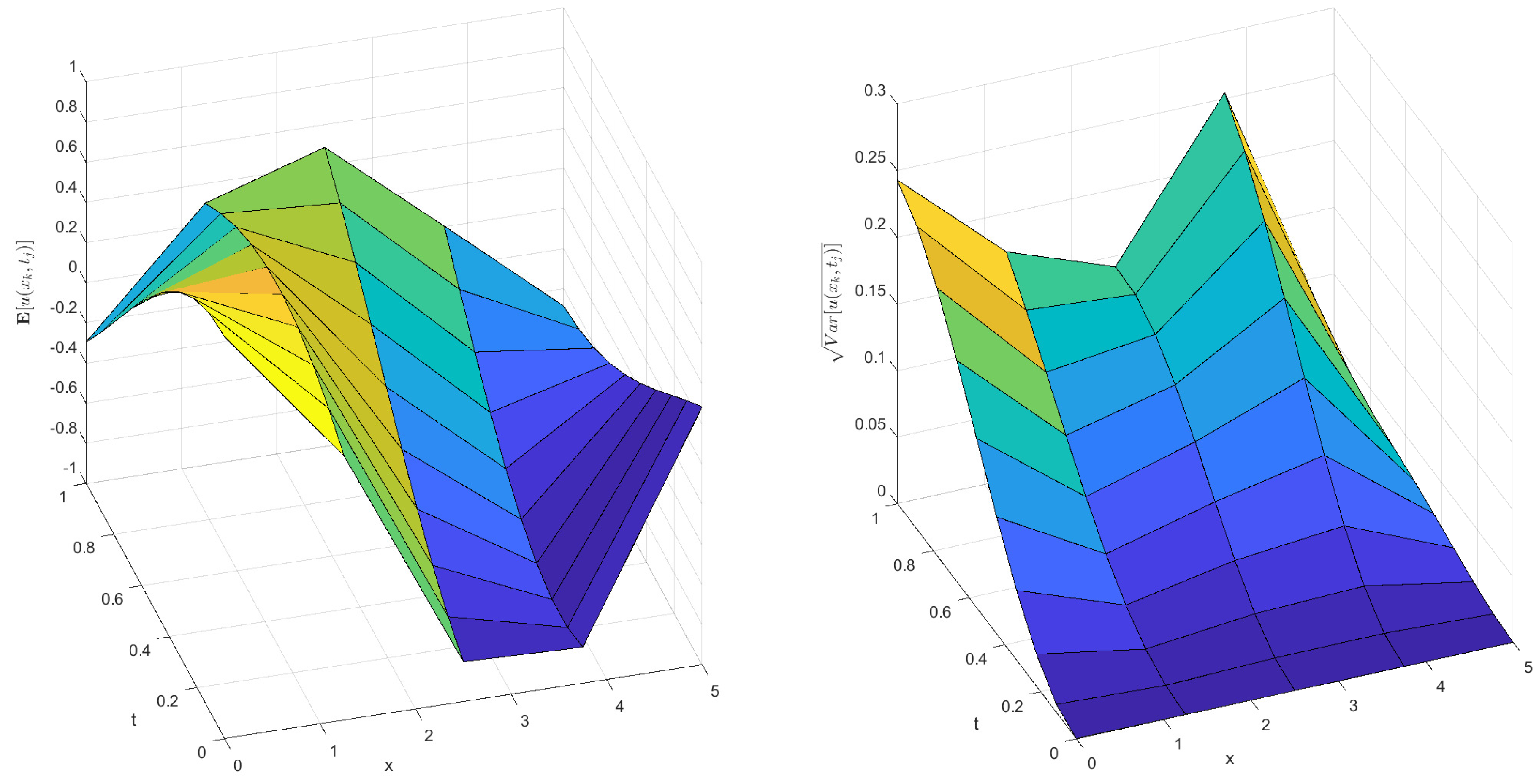
Example 3. We consider a random version of problem (25), with , . In order to approximate the mean and variance of the solutions, the Monte Carlo method with simulations is used. Expectation and variance of the exact solution for the random hyperbolic PDE (
25) are plotted in
Figure 5. As in previous examples, we compare the proposed methods of integration and Laplace inverse in terms of maximum relative error and computational time.
Table 5 presents the results for various
. The CPU-time refers to the total computational time for all
simulations. Note that, for 1000 simulations, the exact solution (
26)–(
27) requires
s to perform the simulations. Thus, Midpoint rule (
,
), Talbot inverse and GL quadrature require less computational time than calculation by the exact formula. As expected, the computational time is increasing with the number of simulations linearly, but errors preserve the order in most cases.
5.4. Random PDE with Non-Constant Coefficients
To complete the study, a random variable coefficient problem is considered.
Example 4. The vibration of the string in is described by Equation (7), subject to the initial conditions and ; and boundary conditions . We set up the parameters: Unlike the deterministic Example 2 with non-constant coefficients where FDM provides a reference analytical solution, reference values are not available here due to the computational complexity that arises in the evaluation of the statistical moments of the approximate stochastic process when time step advances [
18]. A survival reference FDM solution is taking the Monte Carlo method for an appropriate set of realizations. In this case, the number of realizations is
and CPU-time is 16,212 s.
Figure 6 plots the numerical solution. The zero-variance at the boundaries is caused by the boundary conditions. Similar plots are obtained for the considered methods. Thus, we compare them in terms of the maximum relative error, see
Table 6. As it is expected from the previous examples, the most accurate solution is obtained by the midpoint rule and Talbot inverse, although this advantage pays the price of additional computational cost.


