Abstract
In this article, modified techniques, namely the variational iteration transform and Shehu decomposition method, are implemented to achieve an approximate analytical solution for the time-fractional Fornberg–Whitham equation. A comparison is made between the results of the variational iteration transform method and the Shehu decomposition method. The solution procedure reveals that the variational iteration transform method and Shehu decomposition method is effective, reliable and straightforward. The variational iteration transform methods solve non-linear problems without using Adomian’s polynomials and He’s polynomials, which is a clear advantage over the decomposition technique. The solutions achieved are compared with the corresponding exact result to show the efficiency and accuracy of the existing methods in solving a wide variety of linear and non-linear problems arising in various science areas.
1. Introduction
In recent decades, the fractional calculus (FC) implemented in several phenomena in physics, engineering, fluid mechanics, biology and other applied sciences can be defined very effectively using fractional calculus mathematical tools. Fractional derivatives (FDs) provide an excellent tool for describing the hereditary and memory properties of different processes and materials. The FD has occurred in several engineering and sciences problems such as diffusion and reaction processes, frequency-dependent signal processing and system identification, damping behaviour materials, relaxation and creeping for viscoelastic materials [1,2,3,4].
The analysis of nonlinear wave equations and their solutions is of vital significance in several fields of science. Travelling wave ideas are among the most attractive solutions for nonlinear fractional partial differential equations (FPDEs). Nonlinear FPDEs are commonly known as complex physical and mechanical processes. Therefore, it is of great significance to get exact solutions for nonlinear FPDEs, and in general, travelling wave solutions are among the exciting types of solutions for nonlinear FPDEs. On the other hand, other nonlinear FPDEs, such as the Kortewegde-Vries or the Camassa-Holm equations, have been identified to have several moving wave results. These are design equations for nonlinear multi-directional dispersive waves in shallow water [5,6].
The study of the Fornberg–Whitham equation (FWE) is of great importance in many fields of mathematical physics. The Fornberg–Whitham equation [7,8] is given as
The qualitative behavior of wave breakage, a nonlinear dispersive wave equation, appears in the study. The FWE is shown to allow peakon solutions as a numerical simulation for limiting wave heights and the occurrence of wave breaks. In 1978, Fornberg and Whitham achieve a peaked solution of the form , where C is constant. Tian and Zhou [2] have identified the implicit type of wave propagation solutions called antikink-like wave solutions and kink-like wave solutions. The analysis of FWEs by different numerical and analytical methods, such as Laplace decomposition technique [9], Lie Symmetry [10], variational iteration technique [11], differential transformation technique [12], new iterative technique [13], homotopy-perturbation technique [14] and homotopy analysis transform technique [15].
The variational iteration method was first developed by J.H.He and was successfully applied to autonomous ODEs in [16,17]. This technique has been demonstrated to be an effective method for solving different types of problems. Similarly, this method is modified with the Shehu transform method’s help, so the modified technique is called the variational iteration transform method (VITM). Different types of DEs and PDEs have solved VITM. For instance, this technique is used for solving linear fractional differential equations in [18]. This technique is applied in [19] for solving nonlinear oscillator equations. As a benefit of VITM over Adomian’s decomposition process, the former approach provides the problem’s solution without computing Adomian’s polynomials. This system gives a fast solution to the problem while the [20] mesh point methods provide approximation at mesh points. This method is also useful for obtaining an accurate approximation of the exact solution. G. Adomian is the American mathematician who introduced the Adomian decomposition method. It is focused on searching for solutions in the form of a series and on the decomposition of the nonlinear operator into a sequence where the terms are recurrently computed to use Adomian polynomials [21]. This technique is modified with Shehu transformation, so the modified approach is the Shehu decomposition method. This method is applied to the nonhomogeneous fractional differential equations [22,23,24].
The present manuscript is concerned with the analytical solution of time-fractional Fornberg–Whitham equation. The solution of time-fractional Fornberg–Whitham equation is a topic for the researchers since long. Recently the analytical solution of time-fractional Fornberg–Whitham equation is the main focus of the researchers and mathematicians. This was the challenging work to extend or develop the existing techniques for the solution of fractional-order Fornberg–Whitham equation. Many of them have got success and developed innovative techniques to solve fractional-order Fornberg–Whitham equation. In this regard, the current research work is a novel contribution towards the analytical solution of fractional-order Fornberg–Whitham equations. The present research work is conducted in a very simple and straightforward manner to achieve the analytical solutions of the targeted problems with a small amount of numerical calculations. The convergence of the proposed method is trivial. In conclusion the proposed technique are considered to be the sophisticated contribution towards the analytical solution of fractional-order partial differential equations which are frequently arising in science and engineering.
This article has used the Shehu decomposition method and the variational iteration transform method to solve the fractional-order Fornberg–Whitham equation, including Caputo sense in the fractional derivative. The SDM and VITM obtain semi-analytic solutions in the form of series solutions. It simply improves the original problem lucidly, and so one can test the result with high accuracy and convergence.
The outline of this article is as follows. In Section 2, the basic definition of Shehu transform and fractional calculus are discussed. In Section 3, the variational iteration transform method and Shehu decomposition method are discussed. In Section 4, two test examples of fractional-order Fornberg–Whitham equation are given to elucidate the suggested schemes. In Section 5, conclusions of the work.
2. Preliminaries Concepts
In this section of the article, we represent Caputo’s fractional operator to inspect our proposed problem. In addition to this, we will give the basic concept of Shehu transform, inverse Shehu transform and the Shehu transform of nth derivative for further analysis and investigation.
Definition 1.
The Riemann-Liouville fractional integral is given by [25,26]
Definition 2.
The fractional-order derivative Caputo‘s operator of is defined as [25,26]
Definition 3.
Shehu transform is modern and similar to other integral transform described for exponential order functions. In set A, we take a function is represented by [23,24,27]
The Shehu transform which is given by for a function is defined as
The Shehu transform of a function is : then is called the inverse of which is given as
Definition 4.
Consider be the m-th order classical derivative of the function , then its Shehu integral transform is given by the following formula [23,24,27]:
Definition 5.
The fractional order derivatives of Shehu transformation for [23,24,27]
3. The Conceptualization of VITM
In this section discuses the VITM solution for FPDEs.
with the initial condition
where is the Caputo fractional derivative of order , , and , are linear and non-linear functions, respectively, and are source operators.
The Shehu transform is implemented to Equation (9),
Shehu transform the differentiation property is applying, we get
The iterative scheme required the Lagrange multiplier as
A Lagrange multiplier as
using inverse Shehu transformation , Equation (13) can be written as
the initial value can be find as
4. The Conceptualization of SDM
In this section, we discus the SDM solution of FPDEs.
with the initial condition
where is the Caputo fractional derivative of order , and are linear and non-linear functions, respectively, and is source functions.
Apply Shehu transform to Equation (17),
Applying the differentiation property of Shehu transform, we have
SDM solution of infinite series ,
The non-linear terms is given as
The non-linear term can be find with the help of Adomian polynomials. So the Adomian polynomial formula is define as
Using the inverse Shehu transform to Equation (24),
Identify the following terms,
In general for , is define as
5. Implementation of Techniques
Example 1.
Consider the following fractional-order nonlinear Fornberg–Whitham:
with the initial condition
Taking Shehu transform of (27),
Applying inverse Shehu transform
Using ADM procedure, we get
for
for
for
The SDM solution for example (1) is
The simplification of Equation (33)
The approximate solution by VITM.
For
The exact solution of Equation (27) at,
6. Results and Discussion
The present research work aims to find an analytical solution of time-fractional Fornberg–Whitham equations, implemented the efficient analytical methods. The variational iteration transform technique and Shehu decomposition technique are used to solve the targeted problems. To check the validity of the proposed methods, the solution of some illustrative problems are suggested. The solutions graphs are plotted for both fractional and integer-order problems. In Figure 1, (a) the exact and the approximate solution of example 1 at and (b) the analytical solution of different fractional-order of and . In Figure 2, (a) 3d graph of the exact and (b) the SDM and VITM solutions are plotted at . It is observed that the exact, SDM and VITM solutions are in close contact with the exact result of the given problems. Also in Figure 3, (a) the exact and VITM and SDM solutions plot of example 1, (b) are calculated at different fractional-order , and Figure 4 show fractional-order . It is confirmed that VITM and SDM results are in strong agreement with each other. The similar graphical analysis and discussion can be made for the solutions of example 2 in Figure 5, the 3d graph (a) the exact solution and (b) the SDM and VITM solution are discussed at . Also in Figure 6, (a) the exact and VITM and SDM results plot of example 2 and (b) are calculated at different fractional-order . In these graphs, it is investigated that both methods have a sufficient degree of accuracy. In Table 1 the SDM and VITM results are compared in terms of absolute errors for different fractional-order respectively. It has been shown that the proposed techniques have identical accuracy. It is investigated that results of fractional-order problems are convergent to an integer-order result as fractional-order analysis to integer-order. The same phenomenon of convergence of fractional-order solutions towards integral-order solutions is observed.
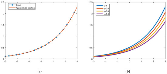
Figure 1.
(a) Exact and approximate solution plot at of example 1. (b) Approximate solution plot of different fractional of example 1.
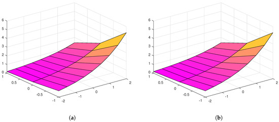
Figure 2.
(a) Exact plot of example 1. (b) Comparison between approximate solution by SDM and VITM plot of example 1 at .
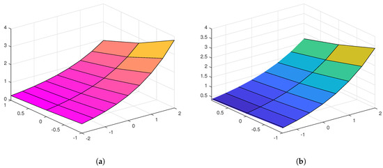
Figure 3.
(a) Comparison between approximate solution by SDM and VITM plot of example 1 at . (b) Comparison between approximate solution by SDM and VITM plot of example 1 at .
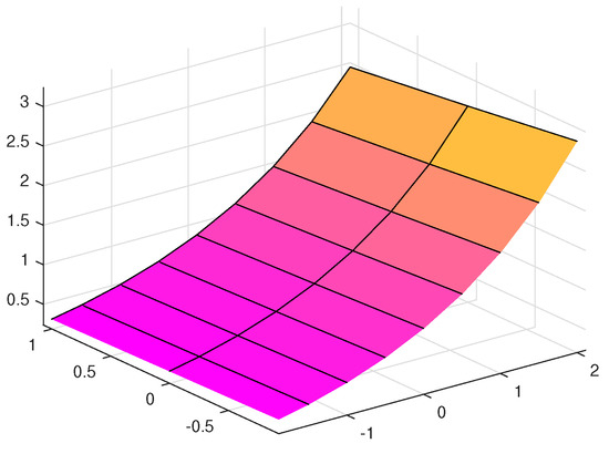
Figure 4.
Comparison between approximate solution by SDM and VITM plot of example 1 at .
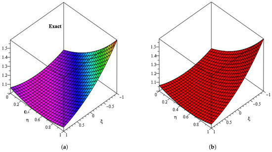
Figure 5.
(a) Exact solution plot of example 2. (b) Comparison between approximate solution by SDM and VITM plot of Example 2 at .
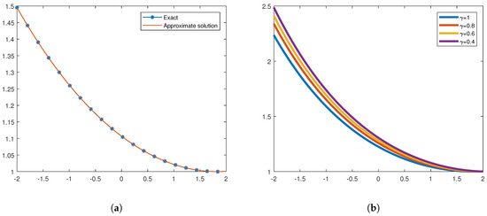
Figure 6.
(a) Exact and approximate solution plot of example 2. (b) Approximate solution plot of different fractional of of example 2.

Table 1.
The comparison between SDM and VITM for the approximate solution of example 1.
7. Conclusions
In this paper, we implemented Shehu decomposition method and variational iteration transform method for solving time-fractional Fornberg–Whitham equation. Some examples of the analytical solution are measured to confirm the accuracy and efficiency of the available method. Graphs and table of the solutions are plotted to show the closed contact between the obtained and exact solutions. The proposed techniques are easier and faster in their concepts and more effective in solving linear and non-linear fractional-order partial differential equation and useful technique for solving a broader class of non-linear fractional models in high precision applied mathematics.
Author Contributions
Conceptualization, N.A.S. and E.R.E.-Z.; methodology, N.A.S.; software, I.D. and E.R.E.-Z.; validation, S.T.; formal analysis, N.A.S. and I.D.; data curation, S.T.; writing–original draft preparation N.A.S.; writing–review and editing, I.D.; supervision, J.D.C.; project administration, N.A.S.; funding acquisition, J.D.C. All authors have read and agreed to the published version of the manuscript.
Funding
This research received no external funding.
Acknowledgments
This work was supported by Korea Institute of Energy Technology Evaluation and Planning (KETEP) grant funded by the Korea government (MOTIE) (No. 20192010107020, Development of hybrid adsorption chiller using unutilized heat source of low temperature). S. Taherifar, would like to express her sincere gratitude to the Research Council of Shahid Chamran University of Ahvaz for its financial support (Grant No. SCU.MC99.29826).
Conflicts of Interest
The authors have no conflict of interest.
References
- Hilfer, R. (Ed.) Applications of Fractional Calculus in Physics; World Scientific: Singapore, 2000; Volume 35, pp. 87–130. [Google Scholar]
- Magin, R.L. Fractional Calculus in Bioengineering; Begell House: Redding, CA, USA, 2006; Volume 2. [Google Scholar]
- Sabatier, J.A.T.M.J.; Agrawal, O.P.; Machado, J.T. Advances in Fractional Calculus; Springer: Dordrecht, The Netherlands, 2007; Volume 4. [Google Scholar]
- Al-luhaibi, M.S. An analytical treatment to fractional Fornberg–Whitham equation. Math. Sci. 2017, 11, 1–6. [Google Scholar] [CrossRef]
- Camacho, J.C.; Rosa, M.; Gandarias, M.L.; Bruzon, M.S. Classical symmetries, travelling wave solutions and conservation laws of a generalized Fornberg–Whitham equation. J. Comput. Appl. Math. 2017, 318, 149–155. [Google Scholar] [CrossRef]
- Bruzon, M.S.; Marquez, A.P.; Garrido, T.M.; Recio, E.; de la Rosa, R. Conservation laws for a generalized seventh order KdV equation. J. Comput. Appl. Math. 2019, 354, 682–688. [Google Scholar] [CrossRef]
- Whitham, G.B. Variational methods and applications to water waves. Proceedings of the Royal Society of London. Series A. Math. Phys. Sci. 1967, 299, 6–25. [Google Scholar]
- Fornberg, B.; Whitham, G.B. A numerical and theoretical study of certain nonlinear wave phenomena. Philosophical Transactions of the Royal Society of London. Ser. A Math. Phys. Sci. 1978, 289, 373–404. [Google Scholar]
- Kumar, D.; Singh, J.; Baleanu, D. A new analysis of the Fornberg–Whitham equation pertaining to a fractional derivative with Mittag-Leffler-type kernel. Eur. Phys. J. Plus 2018, 133, 1–10. [Google Scholar] [CrossRef]
- Hashemi, M.S.; Haji-Badali, A.; Vafadar, P. Group invariant solutions and conservation laws of the Fornberg–Whitham equation. Z. Naturforschung A 2014, 69, 489–496. [Google Scholar] [CrossRef]
- Lu, J. An analytical approach to the Fornberg–Whitham type equations by using the variational iteration method. Comput. Math. Appl. 2011, 61, 2010–2013. [Google Scholar] [CrossRef][Green Version]
- Merdan, M.; Gokdogan, A.; Yildirim, A.; Mohyud-Din, S.T. Numerical simulation of fractional Fornberg–Whitham equation by differential transformation method. Abstr. Appl. Anal. 2012, 2012, 965367. [Google Scholar] [CrossRef]
- Ramadan, M. New Iterative Method for Solving the Fornberg-Whitham Equation and Comparison with Homotopy Perturbation Transform Method. Br. J. Math. Comput. Sci. 2014, 4, 1213–1227. [Google Scholar] [CrossRef]
- Abidi, F.; Omrani, K. Numerical solutions for the nonlinear Fornberg–Whitham equation by He’s methods. Int. J. Mod. Phys. B 2011, 25, 4721–4732. [Google Scholar] [CrossRef]
- Wang, K.; Liu, S. Application of new iterative transform method and modified fractional homotopy analysis transform method for fractional Fornberg–Whitham equation. J. Nonlinear Sci. Appl. 2016, 9, 2419–2433. [Google Scholar] [CrossRef]
- He, J.H. Approximate solution of nonlinear differential equations with convolution product nonlinearities. Comput. Methods Appl. Mech. Eng. 1998, 167, 69–73. [Google Scholar] [CrossRef]
- He, J.H. Variational iteration method for autonomous ordinary differential systems. Appl. Math. Comput. 2000, 114, 115–123. [Google Scholar] [CrossRef]
- Wu, G.C.; Baleanu, D. Variational iteration method for fractional calculus-a universal approach by Laplace transform. Adv. Differ. Equ. 2013, 2013, 1–9. [Google Scholar] [CrossRef]
- Anjum, N.; He, J.H. Laplace transform: Making the variational iteration method easier. Appl. Math. Lett. 2019, 92, 134–138. [Google Scholar] [CrossRef]
- Dehghan, M. Finite difference procedures for solving a problem arising in modeling and design of certain optoelectronic devices. Math. Comput. Simul. 2006, 71, 16–30. [Google Scholar] [CrossRef]
- Adomian, G. Solving Frontier Problems of Physics: The Decomposition Method; Kluwer Academic Publishers: Boston, MA, USA, 1994. [Google Scholar]
- Khalouta, A.; Kadem, A. A New Method to Solve Fractional Differential Equations: Inverse Fractional Shehu Transform Method. Appl. Appl. Math. 2019, 14, 926–941. [Google Scholar]
- Bokhari, A.; Baleanu, D.; Belgacem, R. Application of Shehu transform to Atangana-Baleanu derivatives. J. Math. Comput. Sci. 2019, 20, 101–107. [Google Scholar] [CrossRef]
- Belgacem, R.; Baleanu, D.; Bokhari, A. Shehu Transform and Applications to Caputo-Fractional Differential Equations. Int. J. Anal. Appl. 2019, 17, 917–927. [Google Scholar]
- Machado, J.; Baleanu, D.; Chen, W.; Sabatier, J. New trends in fractional dynamics. J. Vib. Control. SAGE Publ. 2014, 20, 963. [Google Scholar] [CrossRef]
- Baleanu, D.; Guvenc, Z.; Machado, J. New Trends in Nanotechnology and Fractional Calculus Applications; Springer: Dordrecht, The Netherlands, 2010. [Google Scholar]
- Maitama, S.; Zhao, W. New integral transform: Shehu transform a generalization of Sumudu and Laplace transform for solving differential equations. arXiv 2019, arXiv:1904.11370. [Google Scholar]
Publisher’s Note: MDPI stays neutral with regard to jurisdictional claims in published maps and institutional affiliations. |
© 2021 by the authors. Licensee MDPI, Basel, Switzerland. This article is an open access article distributed under the terms and conditions of the Creative Commons Attribution (CC BY) license (http://creativecommons.org/licenses/by/4.0/).