Four-Quadrant Riemann Problem for a 2 × 2 System Involving Delta Shock

Abstract

In this paper, a four-quadrant Riemann problem for a $2\times 2$ system of hyperbolic conservation laws is considered in the case of delta shock appearing at the initial discontinuity. We also remove the restriction in that there is only one planar wave at each initial discontinuity. We include the existence of two elementary waves at each initial discontinuity and classify 14 topologically distinct solutions. For each case, we construct an analytic solution and compute the numerical solution.

1. Introduction

In 1977, in doctoral dissertation (thesis advisor, H. Kranzer), Korchinski [1] considered the Riemann problem (RP) for the system:

$$\left\{\begin{array}{c}{u}_t+{(\frac{1}{2}{u}^2)}_x=0,\hfill \\ v_t+{(\frac{1}{2}uv)}_x=0.\hfill \end{array}\right.$$

(1)

They found that the delta function is supported on a discontinuity, which was motivated by some numerical calculations of the Lax-Friedrich scheme, which was later called a delta shock.

For a hyperbolic system of conservation laws, the four-quadrant RP is the initial value problem:

$$U_t+f{(U)}_x+g{(U)}_y=0$$

(2)

with the initial data $U(x,y,0)=U_i, i=1,\cdots ,4,$ where i denotes the ith quadrant. Here, $U(x,y,t)={\left(u_1(x,y,t),\cdots ,u_n(x,y,t)\right)}^T$ denotes an n-dimensional vector of conserved quantities, and f and g are nonlinear fluxes.

Since Zhang and Zheng’s illuminating conjecture [2] on the classification and structure of the solution of four-quadrant RP for 2-D gas dynamics systems in 1990, many studies have been conducted on simplified gas-dynamics-like models.

In 1994, Tan and Zhang [3,4] studied a four-quadrant RP for a 2-D system:

$$\left\{\begin{array}{c}{u}_t+{(u^2)}_x+{(uv)}_y=0,\hfill \\ v_t+{(uv)}_x+{(v^2)}_y=0.\hfill \end{array}\right.$$

(3)

In a series of papers, they classified and constructed an analytic solution in the case of initial data involving four contact discontinuities ($4J$) [3] and in the case of the initial data involving rarefaction waves [4]. They found the delta shock in this model independently of Korchinski, and Tan et al. [5] established the concept of a delta shock. In addition, Pang et al. [6,7], and Shen [8] considered three constant initial data for the system (3).

Under the assumption that $\rho =const.\equiv 1$, Zhang et al. [9] considered a four-quadrant RP for pressure-gradient equations (4) of the compressible Euler system:

$$\left\{\begin{array}{c}{u}_t+p_x=0,\hfill \\ v_t+p_y=0,\hfill \\ E_t+{(pu)}_x+{(pv)}_y=0,\hfill \end{array}\right.$$

(4)

where p is the pressure, $(u,v)$ is the velocity, and $E=(u^2+v^2)/2+p$ is the energy. Shen and Sun [10] considered the system (4) with the initial data of three constants in three fan domains.

Sheng and Zhang [11] solved a four-quadrant RP for a 2-D system, which is called the transportation equation:

$$\left\{\begin{array}{c}{\rho }_t+{(\rho u)}_x+{(\rho v)}_y=0,\hfill \\ {(\rho u)}_t+{(\rho u^2)}_x+{(\rho uv)}_y=0,\hfill \\ {(\rho v)}_t+{(\rho uv)}_x+{(\rho v^2)}_y=0.\hfill \end{array}\right.$$

(5)

Cheng et al. [12] considered the RP for the zero-pressure gas dynamics model (5) with three constant states, and Mach reflection-like configurations appear in some of the solutions.

The 2-D RP for Chaplygin gas dynamics with three and four constant states were investigated by Wang et al. [13] and Chen and Qu [14], respectively. Shearer [15] studied the RP for $2\times 2$ systems of nonstrictly hyperbolic conservation laws with quadratic nonlinearities that are nondegenerate. In addition, Andrianov and Warnecke [16] considered the RP for compressible duct flows.

Most of the RPs cited above were applied under the following assumption [17]:

(H) Outside a neighborhood of the origin, each jump of the initial data projects exactly one plane elementary wave.

This is a restricted assumption for systems because an $n\times n$ system can generally develop n waves at each initial discontinuity. Most of the RPs citations below were done without the above assumption $(H)$.

In a series of papers [18,19], Hwang and Lindquist solved the 2-D RP of the system (6), which is a generalization of the 1-D Keyfitz–Kranzer–Issacson–Temple model [20,21,22]:

$$\left\{\begin{array}{c}{s}_t+f^A{(s,c)}_x+f^B{(s,c)}_y=0,\hfill \\ {(cs)}_t+{(c{f}^A(s,c))}_x+{(c{f}^B(s,c))}_y=0,\hfill \end{array}\right.$$

(6)

where

$$f^k(s,c)=s^2[1+k(1-c)(1-s)], 0<k<\frac{1}{2}, \mathrm{for}k=A, B.$$

(7)

Under the fundamental assumption of $u=v$, Sun [23] constructed six topologically distinct solutions for a nonstrictly hyperbolic system (8):

$$\left\{\begin{array}{c}{\rho }_t+{(\rho u)}_x+{(\rho u)}_y=0,\hfill \\ u_t+{(\frac{u^2}{2})}_x+{(\frac{u^2}{2})}_y=0.\hfill \end{array}\right.$$

(8)

Shen et al. [24] constructed ten solutions for the system (9):

$$\left\{\begin{array}{c}{u}_t+{(u^2)}_x+{(u^2)}_y=0,\hfill \\ {\rho }_t+{(\rho u)}_x+{(\rho u)}_y=0.\hfill \end{array}\right.$$

(9)

This equation can also be considered to be a simplified gas-dynamics-like model because it can be derived from 2-D isentropic Euler equations [25]. Because this is an isotropic case ($f=g$ in Equation (2)), they considered interactions in the $\eta >\xi$ plane by applying the transformation and symmetry. Hwang et al. [26] considered a 2-D RP with three constant initial data for the system (9). They classified and constructed 12 solutions.

In this paper, our interest is to classify and construct the analytic solution for a $2\times 2$ hyperbolic system (9) in the case of initial four-quadrant data without the assumption $(H)$. We consider Riemann’s initial data involving delta shock. The numerical solution is also computed for comparison with the analytical solution.

We apply the 2-D direct construction method within the entire plane. This approach has certain advantages because the wave interactions in the full plane can be seen, and the constructed analytic solutions can be compared with numerical solutions. The results show extremely interesting structures of wave interactions of the RP, and the numerical solution is remarkably coincident with the constructed analytic solution. Because the theory gives little insight for the qualitative behavior of wave interactions, we need to construct the solution for each system. Furthermore, since general theory does not exist for multidimensional system, 2-D RP for systems must be investigated on a case-by-case basis.

In Section 2, preliminaries, including elementary waves, are presented. In Section 3, the initial data involving the delta shock are formally classified as 52 cases, which results in 14 solutions. We construct analytic and numerical solutions for each case.

2. Preliminaries

The system (9) is changed to a self-similar form

$$\left\{\begin{array}{c}-\xi u_{\xi }-\eta u_{\eta }+{(u^2)}_{\xi }+{(u^2)}_{\eta }=0,\hfill \\ -\xi {\rho }_{\xi }-\eta {\rho }_{\eta }+{(\rho u)}_{\xi }+{(\rho u)}_{\eta }=0,\hfill \end{array}\right.$$

(10)

through $\xi =x/t, \eta =y/t$. The system (10) has two eigenvalues and the corresponding right eigenvectors:

$${\lambda }_1=\frac{u-\eta }{u-\xi }, {\lambda }_2=\frac{2u-\eta }{2u-\xi }, r_1={(0,1)}^T, r_2={(u,\rho )}^T.$$

(11)

Then, the ${\lambda }_1$ field is linearly degenerated and the ${\lambda }_2$ field is genuinely nonlinear if $\eta \ne \xi$ and $u\ne 0$.

From the initial discontinuity between two sides $(u_l,{\rho }_l)$ and $(u_r,{\rho }_r)$ in the counterclockwise direction, we use the notation $R_{lr}, J_{lr}, S_{lr}, S_{{\delta }_{lr}}$ for the rarefaction wave, contact discontinuity, shock, and delta shock, respectively.

From the Rankine–Hugoniot condition, the contact discontinuity satisfies

$$\frac{d\eta }{d\xi }=\frac{\eta -u_l}{\xi -u_l}=\frac{\eta -u_r}{\xi -u_r},$$

(12)

which shows that it is directed to the singular point $(u_l,u_l)=(u_r,u_r)$. Here, $J_{lr}(\xi )$ can be expressed as

$$J_{lr}(\xi ):\xi =u_l=u_r.$$

(13)

Again, from the jump condition, the shock satisfies

$$\frac{d\eta }{d\xi }=\frac{\eta -(u_l+u_r)}{\xi -(u_l+u_r)}, \frac{{\rho }_l}{u_l}=\frac{{\rho }_r}{u_r},$$

(14)

which shows that it directs to the singular point $(u_l+u_r,u_l+u_r)$. The entropy condition is defined as three characteristic ”incoming” lines and the remaining ”outgoing” line. The shock $S_{lr}(\xi )$ can be expressed as follows:

$$\begin{array}{c}{S}_{lr}(\xi ):\xi =u_l+u_r, \frac{{\rho }_l}{u_l}=\frac{{\rho }_r}{u_r},\\ \left(0<u_l<u_r \mathrm{or} u_l<u_r<0 \mathrm{for} \eta >\xi , 0<u_r<u_l \mathrm{or} u_r<u_l<0 \mathrm{for} \eta <\xi \right).\end{array}$$

(15)

Again, from the generalized Rankine–Hugoniot condition, the delta shock is directed to the singular point $(u_l+u_r,u_l+u_r)$. The entropy condition of delta shock implies that all characteristics on both sides of the delta shock are ”non-outgoing” [24]. The delta shock $S_{{\delta }_{lr}}(\xi )$ can be expressed as follows:

$$S_{{\delta }_{lr}}(\xi ):\xi =u_l+u_r, (u_l<0<u_r \mathrm{for} \eta >\xi , u_r<0<u_l \mathrm{for} \eta <\xi ).$$

(16)

The delta shock is described in detail in [3,5,24,27,28].

However, because the second characteristic line satisfies

$$\frac{d\eta }{d\xi }=\frac{\eta -2u}{\xi -2u}$$

(17)

which shows that it directs $(2u,2u)$, $R_{lr}(\xi )$ can be expressed as follows:

$$R_{lr}(\xi ):\xi =2u, \frac{\rho }{u}=\frac{{\rho }_l}{u_l}, \left(u_r\le u\le u_l \mathrm{for} \eta >\xi , u_l\le u\le u_r \mathrm{for} \eta <\xi \right).$$

(18)

Here, (13), (15), (16), and (18) represent the waves that are parallel to the $\eta$-axis. The waves parallel to the $\xi$-axis can be described in a similar manner.

3. Construction of the Solution

We consider a four-quadrant RP for system (9). From the entropy condition, all four characteristics are incoming from both sides of the delta shock. This means that 0 is between the two states. Thus, we must consider the order of $u_1$, $u_2$, $u_3$, $u_4$, and 0 because of delta shock, which brings a total of 5! = 120 cases. The cases including a delta shock are reduced to 52 cases, which resulted in 14 topologically distinct solutions.

Because we remove the assumption $(H)$, there is one or two waves at infinity for each discontinuity. Consider the values of u on either side of the initial discontinuity. If they have the same sign, then we have two waves: a contact shock (JS) or contact rarefaction (JR). If they have different signs, then we have only one wave: $S_{\delta }$ or R.

Because one of the fields of the system (9) is linearly degenerate, contact discontinuity appears as a solution of the RP. For the numerical solution, to reduce the numerical dissipations of the contact discontinuity, the flux functions of the semi-discrete central upwind scheme are modified. Further details can be found in [26,29,30]. In this study, the computational domain is $[-4,4]\times [-4,4]$ and t = 0.2, ${\rho }_i=0.77$ for $i=1,\cdots ,4$. We use 1200 × 1200 cells, and the CFL is 0.05.

3.1. Two Delta Shocks

For the classification of waves at the initial discontinuities, we count the exterior waves that come from the positive $\eta$-axis at first, and then at the axes in the counterclockwise direction. In the classification of the initial data, 21034 and 41032 indicate that $u_2<u_1<0<u_3<u_4$ and $u_4<u_1<0<u_3<u_2$, respectively.

3.1.1. No Shock Wave

The upper and lower sides of the line $\eta =\xi$ form a symmetrical structure in each of the following cases

$$\begin{array}{c}\mathrm{Case}1: \begin{array}{c}JR+S_{\delta }+JR+S_{\delta } (21034), S_{\delta }+RJ+S_{\delta }+RJ (41032)\hfill \end{array}\hfill \\ \mathrm{Case}2: \begin{array}{c}JR+S_{\delta }+S_{\delta }+RJ(24103, 42103), S_{\delta }+RJ+JR+S_{\delta }(10324, 10342)\hfill \end{array}\hfill \\ \mathrm{Case}3: \begin{array}{c}{S}_{\delta }+R+R+S_{\delta } (31024, 31042), R+S_{\delta }+S_{\delta }+R (24031, 42031)\hfill \end{array}\hfill \\ \mathrm{Case}4: \begin{array}{c}{S}_{\delta }+R+R+S_{\delta } (13024, 13042), R+S_{\delta }+S_{\delta }+R (24013, 42013)\hfill \end{array}\hfill \end{array}$$

Case 1.$JR+S_{\delta }+JR+S_{\delta } (u_2<u_1<0<u_3<u_4)$

From the initial discontinuity at the positive $\eta$-axis, the contact $J_{1a}$ and the rarefaction $R_{a2}$ are developed, and a new state $(u_a,{\rho }_a)$ satisfies $u_a=u_1$ and $\frac{{\rho }_a}{u_a}=\frac{{\rho }_2}{u_2}$. Here, $J_{1a}$ is directed to the singular point $(u_1,u_1)$, and the rarefaction $R_{a2}$ is directed to the singular point $(2u,2u)$ for $u_2\le u\le u_1$. From the initial discontinuity at the negative $\xi$-axis, the exterior wave connecting states $(u_2,{\rho }_2)$ and $(u_3,{\rho }_3)$ is $S_{{\delta }_{23}}$ parallel to the negative $\xi$-axis. In addition, $S_{{\delta }_{23}}$ is directed to the singular point $(u_2+u_3,u_2+u_3)$. From the initial discontinuity at the negative $\eta$-axis, $J_{3c}$ and $R_{c4}$ are developed, and a new state $(u_c,{\rho }_c)$ satisfies $u_c=u_3$ and $\frac{{\rho }_c}{u_c}=\frac{{\rho }_4}{u_4}$. Moreover, $J_{3c}$ is directed to the singular point $(u_3,u_3)$, and the rarefaction $R_{c4}$ is directed to $(2u,2u)$ for $u_3\le u\le u_4$. From the initial discontinuity at the positive $\xi$-axis, the exterior wave connecting states $(u_4,{\rho }_4)$ and $(u_1,{\rho }_1)$ is $S_{{\delta }_{41}}$ parallel to the positive $\xi$-axis. Finally, $S_{{\delta }_{41}}$ is directed to the singular point $(u_4+u_1,u_4+u_1)$.

The straight delta shock $S_{{\delta }_{23}}$ completely penetrates the rarefaction wave $R_{a2}$ at point $A(2u_2,u_1+u_2)$, and then the curved delta shock $\eta =\eta (\xi )$ from A to $B(2u_1,\frac{u_1^2+u_3^2-2u_1{u}_2}{u_3-u_2})$ satisfies

$$\frac{d\eta }{d\xi }=\frac{\eta -(u+u_3)}{\xi -(u+u_3)}, \xi =2u, \frac{\rho }{u}=\frac{{\rho }_2}{u_2}, u_2\le u\le u_1,$$

(19)

and we obtain

$$\eta =\xi +\frac{1}{u_3-u_2}{\left(\frac{\xi }{2}-u_3\right)}^2, 2u_2\le \xi \le 2u_1.$$

(20)

This straight delta shock $S_{{\delta }_{a3}}$ meets the contact discontinuity $J_{1a}$ at point $C(u_1,\frac{u_3^2-u_1{u}_2}{u_3-u_2})$ and continues to the singular point $D(u_1+u_3,u_1+u_3)$, and has the form

$$\eta -(u_1+u_3)=\frac{u_1-u_2}{u_3-u_2}(\xi -(u_1+u_3)), 2u_1\le \xi \le u_1+u_3.$$

(21)

By contrast, the delta shock $S_{{\delta }_{41}}$ penetrates the whole rarefaction wave $R_{c4}$, and the straight delta shock $S_{{\delta }_{c1}}$ from the point $E(2u_3,\frac{u_1^2+u_3^2-2u_3{u}_4}{u_1-u_4})$ then meets $J_{3c}$ at the point $F(u_3,\frac{u_1^2-u_3{u}_4}{u_1-u_4})$ and continues to the singular point D. The solutions are provided in Figure 1 and show good agreement. The initial condition is $u_1=-0.15, u_2=-0.37$, $u_3=0.43$, $u_4=0.56.$

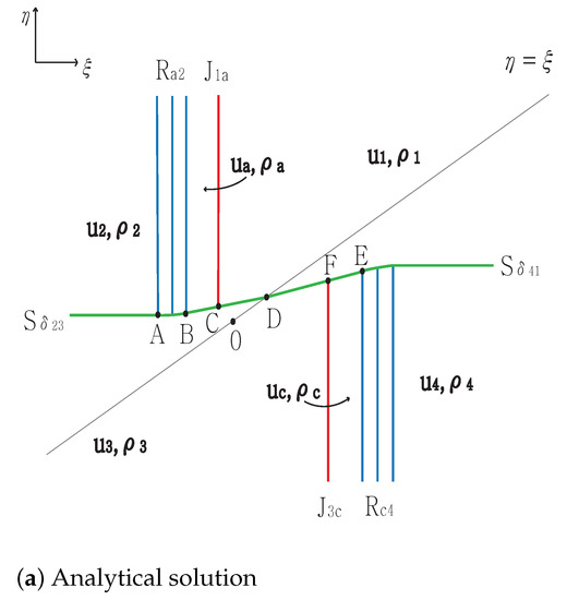
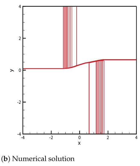
Figure 1. Case 1. $JR+S_{\delta }+JR+S_{\delta }$.

Case 2.$JR+S_{\delta }+S_{\delta }+RJ (u_2<u_4<u_1<0<u_3)$

From the initial discontinuity, a delta shock is formed at the negative $\xi$-axis and negative $\eta$-axis, and contact rarefaction is formed at the positive $\eta$-axis and positive $\xi$-axis. The delta shock $S_{{\delta }_{23}}$ penetrates the entire rarefaction wave $R_{a2}$. The straight delta shock $S_{{\delta }_{a3}}$ from point $A(2u_1,\frac{u_1^2+u_3^2-2u_1{u}_2}{u_3-u_2})$ meets the contact discontinuity $J_{1a}$ at point $C(u_1,\frac{u_1{u}_2-u_3^2}{u_2-u_3})$ and continues to the singular point $B(u_1+u_3,u_1+u_3)$.

By contrast, the delta shock $S_{{\delta }_{34}}$ completely penetrates the rarefaction wave $R_{4d}$. The straight delta shock $S_{{\delta }_{3d}}$ from the point $D(\frac{u_1^2+u_3^2-2u_1{u}_4}{u_3-u_4},2u_1)$ meets the contact discontinuity $J_{d1}$ at point $E(\frac{u_1{u}_4-u_3^2}{u_4-u_3},u_1)$, and then continues to the singular point $B(u_1+u_3,u_1+u_3)$. The solutions are shown in Figure 2. The initial condition for the numerical computation is $u_1=-0.37, u_2=-0.56, u_3=0.15, u_4=-0.43.$

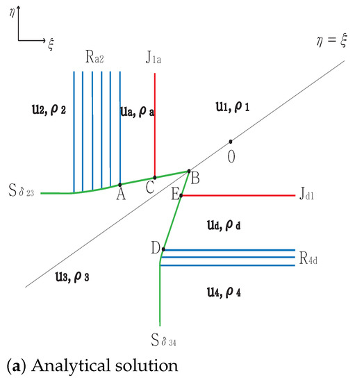
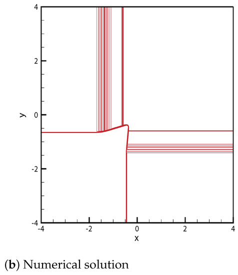
Figure 2. Case 2. $JR+S_{\delta }+S_{\delta }+RJ$.

Case 3.$R+S_{\delta }+S_{\delta }+R (u_2<u_4<0<u_3<u_1)$

In this case, only one wave is formed at each initial discontinuity. From the initial discontinuity at the positive $\eta$-axis, the exterior wave connecting states $(u_1,{\rho }_1)$ and $(u_2,{\rho }_2)$ is the rarefaction $R_{12}$ parallel to the positive $\eta$-axis. The rarefaction $R_{12}$ is directed to $(2u,2u)$ for $u_2\le u\le u_1$. From the initial discontinuity at the negative $\xi$-axis, the exterior wave connecting states $(u_2,{\rho }_2)$ and $(u_3,{\rho }_3)$ is $S_{{\delta }_{23}}$, which is directed to the singular point $(u_2+u_3,u_2+u_3)$. From the initial discontinuity at the negative $\eta$-axis, the exterior wave connecting states $(u_3,{\rho }_3)$ and $(u_4,{\rho }_4)$ is $S_{\delta 34}$, which is directed to the singular point $(u_3+u_4,u_3+u_4)$. From the initial discontinuity at the positive $\xi$-axis, the exterior wave connecting states $(u_4,{\rho }_4)$ and $(u_1,{\rho }_1)$ is the rarefaction $R_{41}$, which is directed to $(2u,2u)$ for $u_4\le u\le u_1$.

The straight delta shock $S_{{\delta }_{23}}$ meets the rarefaction wave $R_{a2}$ at point $A(2u_2,u_1+u_2)$, and the curved delta shock $\eta =\eta (\xi )$ from A to $B(0,\frac{u_3^2}{u_3-u_2})$ then satisfies

$$\frac{d\eta }{d\xi }=\frac{\eta -(u+u_3)}{\xi -(u+u_3)}, \xi =2u, \frac{\rho }{u}=\frac{{\rho }_2}{u_2}, u_2\le u\le 0,$$

(22)

and we obtain

$$\eta =\xi +\frac{1}{u_3-u_2}{\left(\frac{\xi }{2}-u_3\right)}^2, 2u_2\le \xi \le 0.$$

(23)

Simultaneously, a new shock and a new contact discontinuity occur at B. This is an extremely interesting phenomenon in which the delta shock is switched into shock and contact discontinuity. This new shock satisfies the equations in (22) in $0\le u\le u_3$. Similarly, this curved shock has the same form as (23), and continues to $C(2u_3,2u_3)$. In addition, $J_{e3}$ formed at point B ends at the singular point $D(u_3,u_3)$ and satisfies

$$\eta -u_3=\frac{u_2}{u_2-u_3}(\xi -u_3), 0\le \xi \le u_3.$$

(24)

By contrast, $S_{{\delta }_{34}}$ meets $R_{41}$ at the point $E(u_3+u_4,2u_4)$. The curved delta shock continues to point $F(\frac{u_3^2}{u_3-u_4},0)$, and $J_{3e}$ and $S_{eu} (0\le u\le u_3)$ are formed at F. This shock continues to point C, and $J_{3e}$ ends at the singular point D. This contact discontinuity $J_{3e}$ meets the contact discontinuity $J_{e3}$ at point D. Both rarefaction waves $R_{12}$ and $R_{41}$ meet at the same singular point $(2u,2u)$ for $u_3\le u\le u_1$ between C and $G(2u_1,2u_1)$. The solutions are shown in Figure 3. The initial condition is $u_1=0.56, u_2=-0.37$, $u_3=0.43$, $u_4=-0.15.$

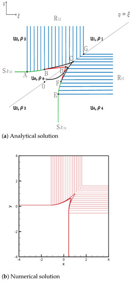
Figure 3. Case 3. $R+S_{\delta }+S_{\delta }+R$.

Case 4.$S_{\delta }+R+R+S_{\delta } (u_1<u_3<0<u_4<u_2)$

As in case 3, only one wave, either a delta shock or rarefaction, is formed at each initial discontinuity. The straight delta shock $S_{{\delta }_{12}}$ meets the rarefaction wave $R_{23}$ at point $A(u_1+u_2,2u_2)$. The curved delta shock continues from A to $B(\frac{u_1^2}{u_1-u_2},0)$. Simultaneously, a new shock and a new contact discontinuity occur at B. This shock formed at point B completely penetrates the rarefaction wave $R_{23}$ from B to $C(\frac{u_1^2+u_3^2-2u_2{u}_3}{u_1-u_2},2u_3)$, and ends at the singular point $D(u_1+u_3,u_1+u_3)$. Here, $J_{1e}$ formed at point B ends at the singular point $E(u_1,u_1)$.

By contrast, $S_{{\delta }_{41}}$ meets $R_{34}$ at the point $F(2u_4,u_4+u_1)$. The curved delta shock continues to point $G(0,\frac{u_1^2}{u_1-u_4})$, and $J_{e1}$ and $S_{ue} (u_3\le u\le 0)$ are formed at G. This shock formed at point G completely penetrates the rarefaction wave $R_{34}$ from G to $H(2u_3,\frac{u_1^2+u_3^2-2u_3{u}_4}{u_1-u_4})$ and ends at the singular point D. In addition, $J_{e1}$ formed at point G ends at the singular point $E(u_1,u_1)$. The solutions are shown in Figure 4. The initial condition is $u_1=-0.37, u_2=0.56, u_3=-0.15, u_4=0.43.$

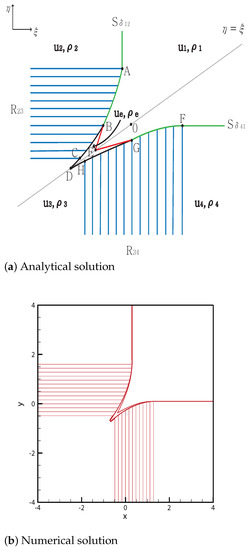
Figure 4. Case 4. $S_{\delta }+R+R+S_{\delta }$.

3.1.2. One Shock Wave

$\begin{array}{c}\mathrm{Case}5: \left\{\begin{array}{c}JS+S_{\delta }+JR+S_{\delta } (12034), S_{\delta }+RJ+S_{\delta }+SJ (14032)\hfill \\ JR+S_{\delta }+JS+S_{\delta } (21043), S_{\delta }+SJ+S_{\delta }+RJ (41023)\hfill \end{array}\right.\hfill \\ \mathrm{Case}6: \left\{\begin{array}{c}JR+S_{\delta }+S_{\delta }+SJ (21403), JS+S_{\delta }+S_{\delta }+RJ (41203)\hfill \\ S_{\delta }+SJ+JR+S_{\delta } (10234), S_{\delta }+RJ+JS+S_{\delta } (10432)\hfill \end{array}\right.\hfill \end{array}$

Case 5.$S_{\delta }+RJ+S_{\delta }+SJ (u_1<u_4<0<u_3<u_2)$

From the initial discontinuity, a delta shock is formed at the positive $\eta$-axis and negative $\eta$-axis, and the rarefaction-contact and shock-contact are formed at the negative $\eta$-axis and positive $\xi$-axis, respectively. The delta shock $S_{{\delta }_{12}}$ completely penetrates the rarefaction wave $R_{2b}$. The straight delta shock $S_{{\delta }_{1b}}$ from the point $A(\frac{u_1^2+u_3^2-2u_2{u}_3}{u_1-u_2},2u_3)$ meets the contact discontinuity $J_{b3}$ at point $C(\frac{u_2{u}_3-u_1^2}{u_2-u_1},u_3)$, and then continues to the singular point $B(u_1+u_3,u_1+u_3)$.

By contrast, the delta shock $S_{{\delta }_{34}}$ intersects with the shock $S_{4d}$ at point $D(u_3+u_4,u_4+u_1)$. Then, the new delta shock $S_{{\delta }_{3d}}$ from D to B satisfies

$$\eta -(u_1+u_3)=\frac{u_3-u_4}{u_1-u_4}(\xi -(u_1+u_3)), u_1+u_3\le \xi \le u_3+u_4.$$

(25)

The straight delta shock $S_{{\delta }_{3d}}$ meets the contact discontinuity $J_{d1}$ at point $E(\frac{u_1{u}_4-u_3^2}{u_4-u_3},u_1)$ and continues to the singular point B. The solutions are shown in Figure 5. The initial condition is $u_1=-0.37, u_2=0.56, u_3=0.43, u_4=-0.15.$

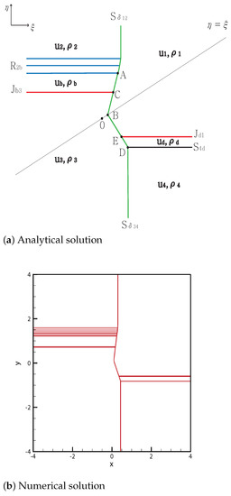
Figure 5. Case 5. $S_{\delta }+RJ+S_{\delta }+SJ$.

Case 6.$JS+S_{\delta }+S_{\delta }+RJ (u_4<u_1<u_2<0<u_3)$

From the initial discontinuity, a delta shock is formed at the negative $\xi$-axis and negative $\eta$-axis, and contact shock and contact rarefaction contact are formed at the positive $\eta$-axis and positive $\xi$-axis, respectively. The delta shock $S_{{\delta }_{23}}$ meets the shock $S_{a2}$ at point $A(u_1+u_2,u_2+u_3)$. The new delta shock $S_{{\delta }_{a3}}$ formed at A meets the contact discontinuity $J_{1a}$ at $C(u_1,\frac{u_1{u}_2-u_3^2}{u_2-u_3})$ and continues to the singular point $B(u_1+u_3,u_1+u_3)$.

By contrast, the delta shock $S_{{\delta }_{34}}$ penetrates the entire rarefaction wave $R_{4d}$, and the straight delta shock $S_{{\delta }_{3d}}$ from the point $D(\frac{u_1^2+u_3^2-2u_1{u}_4}{u_3-u_4},2u_1)$ then meets the contact discontinuity $J_{d1}$ at the point $E(\frac{u_1{u}_4-u_3^2}{u_4-u_3},u_1)$ and continues to the singular point $B(u_1+u_3,u_1+u_3)$. The solutions are shown in Figure 6. The initial condition is $u_1=-0.43,$ $u_2=-0.37,$ $u_3=0.15,$ $u_4=-0.56.$

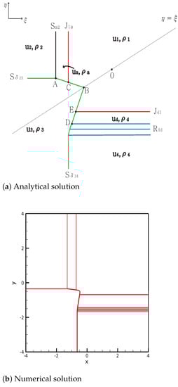
Figure 6. Case 6. $JS+S_{\delta }+S_{\delta }+RJ$.

3.1.3. Two Shock Waves

$\begin{array}{c}\mathrm{Case}7: \begin{array}{c}JS+S_{\delta }+JS+S_{\delta } (12043), S_{\delta }+SJ+S_{\delta }+SJ (14023)\hfill \end{array}\hfill \\ \mathrm{Case}8: \begin{array}{c}JS+S_{\delta }+S_{\delta }+SJ (12403, 14203), S_{\delta }+SJ+JS+S_{\delta } (10243, 10423)\hfill \end{array}\hfill \end{array}$

Case 7.$JS+S_{\delta }+JS+S_{\delta } (u_1<u_2<0<u_4<u_3)$

From the initial discontinuity, a delta shock is formed at the negative $\xi$-axis and positive $\xi$-axis, and a contact shock is formed at the positive $\eta$-axis and negative $\eta$-axis. The delta shock $S_{{\delta }_{23}}$ meets the shock $S_{a2}$ at point $A(u_1+u_2,u_2+u_3)$. The new delta shock $S_{{\delta }_{a3}}$ formed at A meets the contact discontinuity $J_{1a}$ at $C(u_1,\frac{u_1{u}_2-u_3^2}{u_2-u_3})$ and continues to the singular point $B(u_1+u_3,u_1+u_3)$ without changing the direction because $u_a=u_1$.

However, the delta shock $S_{{\delta }_{41}}$ intersects with the shock $S_{c4}$ at the point $D(u_3+u_4,u_4+u_1)$. The new delta shock $S_{{\delta }_{c1}}$ formed at D meets the contact discontinuity $J_{3c}$ at the point $E(u_3,\frac{u_3{u}_4-u_1^2}{u_4-u_1})$ and continues to the singular point $B(u_1+u_3,u_1+u_3)$. The solutions are shown in Figure 7. The initial condition is $u_1=-0.37, u_2=-0.15, u_3=0.56, u_4=0.43.$

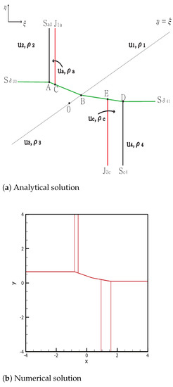
Figure 7. Case 7. $JS+S_{\delta }+JS+S_{\delta }$.

Case 8. $JS+S_{\delta }+S_{\delta }+SJ (u_1<u_2<u_4<0<u_3)$

From the initial discontinuity, a delta shock is formed at the negative $\xi$-axis and negative $\eta$-axis, and a contact shock is formed at the positive $\eta$-axis and positive $\xi$-axis. The delta shock $S_{{\delta }_{23}}$ meets the shock $S_{a2}$ at point $A(u_1+u_2,u_2+u_3)$. The new delta shock $S_{{\delta }_{a3}}$ formed at A meets the contact discontinuity $J_{1a}$ at $C(u_1,\frac{u_1{u}_2-u_3^2}{u_2-u_3})$ and continues to the singular point $B(u_1+u_3,u_1+u_3)$.

By contrast, the delta shock $S_{{\delta }_{34}}$ intersects with the shock $S_{4d}$ at point $D(u_3+u_4,u_4+u_1)$. The new delta shock $S_{{\delta }_{3d}}$ formed at D meets the contact discontinuity $J_{d1}$ at $E(u_3,\frac{u_3{u}_4-u_1^2}{u_4-u_1})$ and continues to the singular point $B(u_1+u_3,u_1+u_3)$. The solutions are shown in Figure 8. The initial condition is $u_1=-0.56, u_2=-0.43, u_3=0.15, u_4=-0.37.$

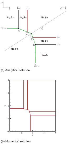
Figure 8. Case 8. $JS+S_{\delta }+S_{\delta }+SJ$.

3.2. One Delta Shock

3.2.1. No Shock Wave

$\mathrm{Case}9: \left\{\begin{array}{c}JR+JR+R+S_{\delta } (32104), S_{\delta }+R+RJ+RJ (34102)\hfill \\ R+S_{\delta }+JR+JR (20341), RJ+RJ+S_{\delta }+R (40321)\hfill \end{array}\right.$

Case 9. $R+S_{\delta }+JR+JR (u_2<0<u_3<u_4<u_1)$

From the initial discontinuity at the positive $\eta$-axis, the exterior wave connecting states $(u_1,{\rho }_1)$ and $(u_2,{\rho }_2)$ is the rarefaction $R_{12}$. The rarefaction $R_{12}$ is directed toward $(2u,2u)$ for $u_2\le u\le u_1$. From the initial discontinuity at the negative $\xi$-axis, the exterior wave connecting states $(u_2,{\rho }_2)$ and $(u_3,{\rho }_3)$ is the delta shock $S_{{\delta }_{23}}$. The delta shock $S_{{\delta }_{23}}$ is directed to the singular point $(u_2+u_3,u_2+u_3)$. From the initial discontinuity at the negative $\eta$-axis, the contact discontinuity $J_{3c}$ and rarefaction $R_{c4}$ and $(u_c,{\rho }_c)$ between $J_{3c}$ and $R_{c4}$ satisfy $u_c=u_3$ and $\frac{{\rho }_c}{u_c}=\frac{{\rho }_4}{u_4}$. Here, $J_{3c}$ is directed toward the singular point $(u_3,u_3)$, and the rarefaction $R_{c4}$ is directed toward $(2u,2u)$ for $u_3\le u\le u_4$. From the initial discontinuity at the positive $\xi$-axis, the contact discontinuity $J_{4d}$ and the rarefaction $R_{d1}$ and a new state $(u_d,{\rho }_d)$ between $J_{4d}$ and $R_{d1}$ are formed. The state $(u_d,{\rho }_d)$ satisfies $u_d=u_4$ and $\frac{{\rho }_d}{u_d}=\frac{{\rho }_1}{u_1}$. In addition, $J_{4d}$ is directed toward the singular point $(u_4,u_4)$, and the rarefaction $R_{d1}$ is directed toward $(2u,2u)$ for $u_4\le u\le u_1$. The delta shock $S_{{\delta }_{23}}$ meets the rarefaction wave $R_{12}$ at point $(2u_2,u_2+u_3)$. Then, a curved delta shock continues toward point $A(0,\frac{u_3^2}{u_3-u_2})$. Simultaneously, $J_{e3}$ and $S_{ue} (0\le u\le u_3)$ are formed at A. This curved shock continues toward point $B(2u_3,2u_3)$, and $J_{e3}$ ends at the singular point $C(u_3,u_3)$. By contrast, both $R_{12}$ and $R_{c4}$ meet at $(2u,2u)$ for $u_3\le u\le u_4$ between $B(2u_3,2u_3)$ and $D(2u_4,2u_4)$. In addition, $J_{4d}$ penetrates the entire rarefaction wave, $R_{c4}$. The straight contact discontinuity continues from $(2u_3,\frac{2u_3{u}_4-u_3^2}{u_4})$ toward $C(u_3,u_3)$. Consequently, three contact discontinuities $J_{e3}, J_{3c}$, and $J_{ce}$ meet at their singular point C. Both rarefaction waves $R_{12}$ and $R_{d1}$ meet at $(2u,2u)$ for $u_4\le u\le u_1$ between D and $E(2u_1,2u_1)$. The solutions are shown in Figure 9. The initial condition is $u_1=0.56, u_2=-0.15, u_3=0.37, u_4=0.43.$

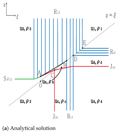
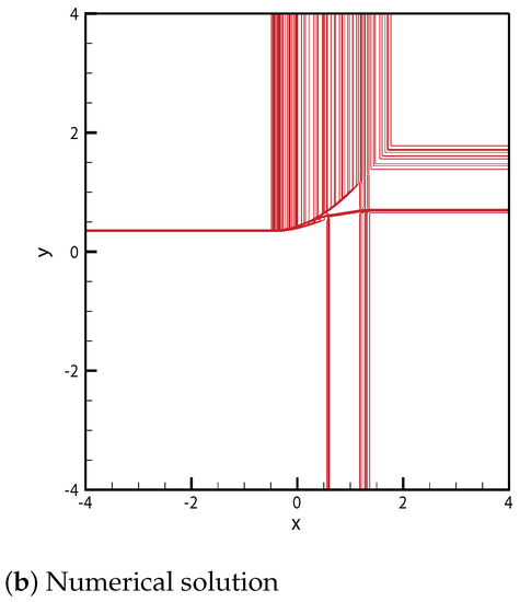
Figure 9. Case 9. $R+S_{\delta }+JR+JR$.

3.2.2. One Shock Wave

$\begin{array}{c}\mathrm{Case}10: \left\{\begin{array}{c}JS+JR+R+S_{\delta } (13204), S_{\delta }+R+RJ+SJ (13402)\hfill \\ R+S_{\delta }+JS+JR (20413), RJ+SJ+S_{\delta }+R (40213)\hfill \end{array}\right.\hfill \\ \mathrm{Case}11: \left\{\begin{array}{c}JS+JR+R+S_{\delta } (31204), S_{\delta }+R+RJ+SJ (31402)\hfill \\ R+S_{\delta }+JS+JR (20431), RJ+SJ+S_{\delta }+R (40231)\hfill \end{array}\right.\hfill \\ \mathrm{Case}12: \left\{\begin{array}{c}JR+JS+R+S_{\delta } (21304), S_{\delta }+R+SJ+RJ (41302)\hfill \\ R+S_{\delta }+JR+JS (20134), SJ+RJ+S_{\delta }+R (40132)\hfill \end{array}\right.\hfill \\ \mathrm{Case}13: \left\{\begin{array}{c}JR+JS+R+S_{\delta } (23104), S_{\delta }+R+SJ+RJ (43102)\hfill \\ R+S_{\delta }+JR+JS (20314), SJ+RJ+S_{\delta }+R (40312)\hfill \end{array}\right.\end{array}$

Case 10.$S_{\delta }+R+RJ+SJ (u_1<u_3<u_4<0<u_2)$

From the initial discontinuity, a delta shock is formed at the positive $\eta$-axis, and a rarefaction is formed at the negative $\xi$-axis, and the rarefaction-contact and shock-contact are formed at the negative $\eta$-axis and positive $\xi$-axis, respectively. The delta shock $S_{{\delta }_{12}}$ meets the rarefaction wave $R_{23}$ at point $A(u_1+u_2,2u_2)$. Then, the curved delta shock continues toward point $B(\frac{u_1^2}{u_1-u_2},0)$. A new shock and a new contact discontinuity are formed at B, and this curved shock ends at point $C(\frac{u_1^2+u_3^2-2u_2{u}_3}{u_1-u_2},2u_3)$. Then, $S_{e3}$ continues from point C to $D(u_1+u_3,u_1+u_3)$, and $J_{1e}$ continues from point B to point $E(u_1,u_1)$. By contrast, $J_{c4}$ intersects with $S_{4d}$ at point $F(u_4,u_4+u_1)$ and the new contact discontinuity $J_{ed}$ from F ends at their singular point E, which equals the singular point of $J_{d1}$ and $J_{1e}$. Therefore, the three contact discontinuities meet at the singular point E. The shock $S_{ce}(=S_{4d})$ completely penetrates $R_{3c}$ and then stops at the singular point D. The solutions are shown in Figure 10. The initial condition is $u_1=-0.73, u_2=0.15, u_3=-0.56$, $u_4=-0.25.$

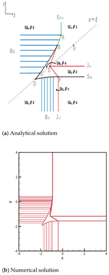
Figure 10. Case 10. $S_{\delta }+R+RJ+SJ$.

Case 11.$R+S_{\delta }+JS+JR (u_2<0<u_4<u_3<u_1)$

From the initial discontinuity, rarefaction is formed at the positive $\eta$-axis, and a delta shock is formed at the negative $\xi$-axis, and contact shock and contact rarefaction are formed at the negative $\eta$-axis and positive $\xi$-axis, respectively. The delta shock $S_{{\delta }_{23}}$ meets the rarefaction wave $R_{12}$ at point $A(2u_2,u_2+u_3)$, and the curved delta shock continues toward point $B(0,\frac{u_3^2}{u_3-u_2})$. Simultaneously, $S_{ue} (0\le u\le u_3)$ and $J_{e3}$ occur at B. The curved shock continues from B toward $C(2u_3,2u_3)$. In addition, $J_{e3}$ formed at point B ends at the singular point $D(u_3,u_3)$.

By contrast, $J_{4d}$ meets $S_{c4}$ at point $E(u_3+u_4,u_4)$ and $J_{ce}$ at the singular point D. Therefore, three contact discontinuities $J_{e3}, J_{3c}$, and $J_{ce}$ meet at their singular point D. The shock $S_{ed}(=S_{c4})$ meets the rarefaction wave $R_{d1}$ at point $F(u_3+u_4,2u_4)$, and the curved shock continues toward C. Both rarefaction waves $R_{12}$ and $R_{d1}$ meet at $(2u,2u)$ for $u_3\le u\le u_1$ between C and $G(2u_1,2u_1)$. The solutions are shown in Figure 11. The initial condition is $u_1=0.56, u_2=-0.15, u_3=0.43, u_4=0.21.$

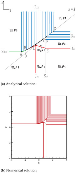
Figure 11. Case 11. $R+S_{\delta }+JS+JR$.

Case 12.$S_{\delta }+R+SJ+RJ (u_4<u_1<u_3<0<u_2)$

From the initial discontinuity, a delta shock is formed at the positive $\eta$-axis and rarefaction is formed at the negative $\xi$-axis; in addition, shock-contact and rarefaction-contact are formed at the negative $\eta$-axis and positive $\xi$-axis, respectively. The straight delta shock $S_{{\delta }_{12}}$ meets $R_{23}$, and then a curved delta shock continues toward $A(\frac{u_1^2}{u_1-u_2},0)$. The new shock formed at A completely penetrates $R_{23}$ and stops at the singular point $B(u_1+u_3,u_1+u_3)$. Moreover, $J_{1e}$ formed at point A ends at the singular point $C(u_1,u_1)$. However, the shock $S_{3c}$ completely penetrates the rarefaction wave $R_{4d}$ from D to the point $E(\frac{u_1^2+u_3^2-2u_1{u}_4}{u_3-u_4},2u_1)$ and it stops at the singular point B. In addition, $J_{c4}$ completely penetrates $R_{ce}(=R_{4d})$ from $F(u_4,2u_4)$ to G and satisfies

$$\frac{d\eta }{d\xi }=\frac{\eta -u}{\xi -u}, \eta =2u, \frac{\rho }{u}=\frac{{\rho }_4}{u_4}, u_4\le u\le u_1.$$

(26)

which gives

$$\xi =\eta -\frac{{\eta }^2}{4u_4}, 2u_4\le \eta \le 2u_1.$$

(27)

The straight contact discontinuity $J_{ed}$ continues from $G(\frac{2u_1{u}_4-u_1^2}{u_4},2u_1)$ to C, satisfying

$$\eta -u_1=\frac{u_4}{u_4-u_1}(\xi -u_1), 2u_1\le \eta \le u_1.$$

(28)

Here, $J_{ed}$ meets $J_{1e}$ and $J_{d1}$ at their singular point C. The solutions are shown in Figure 12. The initial condition is $u_1=-0.43, u_2=0.15, u_3=-0.37, u_4=-0.56.$

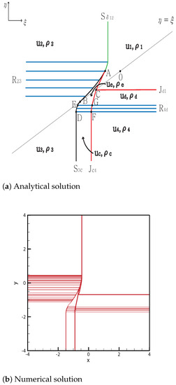
Figure 12. Case 12. $S_{\delta }+R+SJ+RJ$.

Case 13.$S_{\delta }+R+SJ+RJ (u_4<u_3<u_1<0<u_2)$

In this case, the exterior waves at the initial discontinuity are exactly the same as those in case 12. The upper structures are also extremely similar to those in the previous case.

By contrast, both $R_{23}$ and $R_{4d}$ meet at $(2u,2u)$ for $u_3\le u\le u_1$ between $B(2u_1,2u_1)$ and $D(2u_3,2u_3)$. The shock $S_{3c}$ meets $R_{4d}$ at $(u_3+u_4,2u_4)$, and the curved shock then continues toward point D. Here, $J_{c4}$ penetrates the entire rarefaction $R_{4d}$ and the straight contact discontinuity continues from $(\frac{2u_1{u}_4-u_1^2}{u_4},2u_1)$ to $C(u_1,u_1)$, which is a singular point of three contact discontinuities $J_{1e}, J_{d1}$, and $J_{ed}$. In case 12, the shock $S_{3c}$ completely penetrates the rarefaction $R_{4d}$, but $S_{3c}$ partially penetrates $R_{4d}$ in case 13. This difference makes them topologically distinct. The solutions are shown in Figure 13. The initial condition is $u_1=-0.37, u_2=0.15, u_3=-0.43, u_4=-0.56.$

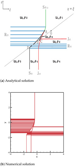
Figure 13. Case 13. $S_{\delta }+R+SJ+RJ$.

3.2.3. Two Shock Waves

$\mathrm{Case}14: \left\{\begin{array}{c}JS+JS+R+S_{\delta } (12304), S_{\delta }+R+SJ+SJ (14302)\hfill \\ R+S_{\delta }+JS+JS (20143), SJ+SJ+S_{\delta }+R (40123)\hfill \end{array}\right.$

Case 14. $JS+JS+R+S_{\delta } (u_1<u_2<u_3<0<u_4)$

From the initial discontinuity, a contact shock is formed at the positive $\eta$-axis and negative $\xi$-axis, and rarefaction and delta shock are formed at the negative $\eta$-axis and positive $\xi$-axis, respectively. In addition, $J_{2b}$ intersects with $S_{a2}$ at point $P(u_1+u_2,u_2)$ and the new contact discontinuity $J_{ae}$ occurs from P to $A(u_1,u_1)$. The shock $S_{a2}(=S_{eb})$ continues from P without changing the direction because $u_e=u_a$ and $u_b=u_2$. This shock $S_{eb}$ meets the shock $S_{b3}$ at the point $Q(u_1+u_2,u_2+u_3)$, and the new shock $S_{e3}$ is formed at Q and ends at the singular point $H(u_1+u_3,u_1+u_3)$. By contrast, $S_{{\delta }_{41}}$ meets $R_{34}$ at the point $R(2u_4,u_4+u_1)$, and the curved delta shock is then from R to $S(0,\frac{u_1^2}{u_1-u_4})$. Simultaneously, $J_{e1}$ and $S_{ue} (u_3\le u\le 0)$ are formed at S. The curved shock from S to T and the straight shock continues from the point $T(2u_3,\frac{u_1^2+u_3^2-2u_3{u}_4}{u_1-u_4})$ and meets $S_{e3}$ at the singular point $H(u_1+u_3,u_1+u_3)$. However, the new contact discontinuity $J_{e1}$ is from S to A and meets two contact discontinuities $J_{1a}$ and $J_{ae}$ at their singular point $A(u_1,u_1)$. The solutions are shown in Figure 14. The initial condition is $u_1=-0.56, u_2=-0.43,$ $u_3=-0.37,$ $u_4=0.15.$

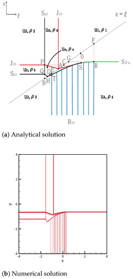
Figure 14. Case 14. $JS+JS+R+S_{\delta }$.

References

- Korchinski, D.J. Solutions of a Riemann Problem for a 2 × 2 System of Conservation Laws Possessing No Classical Weak Solutions. Ph.D. Thesis, Adelphi University, New York, NY, USA, 1977. [Google Scholar]
- Zhang, T.; Zheng, Y.X. Conjecture on the structure of solutions of the Riemann problem for two-dimensional gas dynamics systems. SIAM J. Math. Anal. 1990, 21, 593–630. [Google Scholar] [CrossRef]
- Tan, D.C.; Zhang, T. Two-dimensional Riemann problem for a hyperbolic system of nonlinear conservation laws: I. four-J cases. J. Differ. Equ. 1994, 111, 203–254. [Google Scholar] [CrossRef]
- Tan, D.C.; Zhang, T. Two-dimensional Riemann problem for a hyperbolic system of nonlinear conservation laws: II. Initial data involving some rarefaction waves. J. Differ. Equ. 1994, 111, 255–282. [Google Scholar] [CrossRef]
- Tan, D.C.; Zhang, T.; Chang, T.; Zheng, Y. Delta-shock waves as limits of vanishing viscosity for hyperbolic systems of conservation laws. J. Differ. Equ. 1994, 112, 1–32. [Google Scholar] [CrossRef]
- Pang, Y.; Tian, J.P.; Yang, H. Two-dimensional Riemann problem for a hyperbolic system of conservation laws in three pieces. Appl. Math. Comput. 2012, 219, 1695–1711. [Google Scholar] [CrossRef]
- Pang, Y.; Tian, J.P.; Yang, H. Two-dimensional Riemann problem involving three J’s for a hyperbolic system of nonlinear conservation laws. Appl. Math. Comput. 2013, 219, 4614–4624. [Google Scholar] [CrossRef]
- Shen, C. Riemann problem for a two-dimensional quasilinear hyperbolic system. Electron. J. Differ. Equ. 2015, 2015, 1–13. [Google Scholar]
- Zhang, P.; Li, J.; Zhang, T. On two-dimensional Riemann problem for pressure-gradient equations of the Euler system. Discret. Contin. Dyn. Syst. 1998, 4, 609–634. [Google Scholar] [CrossRef]
- Shen, C.; Sun, M. The Riemann problem for the pressure-gradient system in three pieces. Appl. Math. Lett. 2009, 22, 453–458. [Google Scholar] [CrossRef][Green Version]
- Sheng, W.; Zhang, T. The Riemann Problem for the Transportation Equations in Gas Dynamics; American Mathematical Soc.: Providence, RI, USA, 1999; Volume 654. [Google Scholar]
- Cheng, H.; Liu, W.; Yang, H. Two-dimensional Riemann problems for zero-pressure gas dynamics with three constant states. J. Math. Anal. Appl. 2008, 343, 127–140. [Google Scholar] [CrossRef][Green Version]
- Wang, G.; Chen, B.; Hu, Y. The two-dimensional Riemann problem for Chaplygin gas dynamics with three constant states. J. Math. Anal. Appl. 2012, 393, 544–562. [Google Scholar] [CrossRef]
- Chen, T.; Qu, A. Two-dimensional Riemann problem for Chaplygin gas dynamics in four pieces. J. Math. Anal. Appl. 2017, 448, 580–597. [Google Scholar] [CrossRef]
- Shearer, M. The Riemann problem for 2 × 2 systems of hyperbolic conservation laws with case I quadratic nonlinearities. J. Differ. Equations 1989, 80, 343–363. [Google Scholar] [CrossRef]
- Andrianov, N.; Warnecke, G. On the solution to the Riemann problem for the compressible duct flow. SIAM J. Appl. Math. 2004, 64, 878–901. [Google Scholar]
- Yang, H. Generalized plane delta-shock waves for n-dimensional zero-pressure gas dynamics. J. Math. Anal. Appl. 2001, 260, 18–35. [Google Scholar] [CrossRef]
- Hwang, W.; Lindquist, W.B. The 2-dimensional Riemann problem for a 2 × 2 hyperbolic conservation law I. Isotropic media. SIAM J. Math. Anal. 2002, 34, 341–358. [Google Scholar] [CrossRef]
- Hwang, W.; Lindquist, W.B. The 2-dimensional Riemann problem for a 2 × 2 hyperbolic conservation law II. Anisotropic media. SIAM J. Math. Anal. 2002, 34, 359–384. [Google Scholar] [CrossRef]
- Isaacson, E.L. Global solution of a Riemann Problem for a Non-Strictly Hyperbolic System of Conservation Laws Arising in Enhanced Oil Recovery; Enhanced Oil Recovery Institute, University of Wyoming: Laramie, WY, USA, 1989. [Google Scholar]
- Keyfitz, B.L.; Kranzer, H.C. A system of non-strictly hyperbolic conservation laws arising in elasticity theory. Arch. Ration. Mech. Anal. 1980, 72, 219–241. [Google Scholar] [CrossRef]
- Temple, B. Global solution of the Cauchy problem for a class of 2 × 2 nonstrictly hyperbolic conservation laws. Adv. Appl. Math. 1982, 3, 335–375. [Google Scholar] [CrossRef]
- Sun, M. Construction of the 2D Riemann solutions for a nonstrictly hyperbolic conservation law. Bull. Korean Math. Soc. 2013, 50, 201–216. [Google Scholar] [CrossRef]
- Shen, C.; Sun, M.; Wang, Z. Global structure of Riemann solutions to a system of two-dimensional hyperbolic conservation laws. Nonlinear Anal. 2011, 74, 4754–4770. [Google Scholar] [CrossRef]
- Li, S.; Shen, C. Measure-Valued Solutions to a Non-Strictly Hyperbolic System with Delta-Type Riemann Initial Data. Int. J. Nonlinear Sci. Numer. Simul. 2020, 21, 1. [Google Scholar] [CrossRef]
- Hwang, J.; Shin, M.; Shin, S.; Hwang, W. Two dimensional Riemann problem for a 2 × 2 system of hyperbolic conservation laws involving three constant states. Appl. Math. Comput. 2018, 321, 49–62. [Google Scholar] [CrossRef]
- Keyfitz, B.L.; Kranzer, H.C. Spaces of weighted measures for conservation laws with singular shock solutions. J. Differ. Equ. 1995, 118, 420–451. [Google Scholar] [CrossRef]
- Li, J.; Zhang, T.; Yang, S. The Two-Dimensional Riemann Problem in Gas Dynamics; Longman; Chapman and Hall/CRC: Boca Raton, FL, USA, 1998; Volume 98. [Google Scholar]
- Kurganov, A.; Lin, C.T. On the reduction of numerical dissipation in central-upwind schemes. Commun. Comput. Phys. 2007, 2, 141–163. [Google Scholar]
- Shin, M.; Shin, S.; Hwang, W. A treatment of contact discontinuity for central upwind scheme by changing flux functions. J. Korean Soc. Ind. Appl. Math. 2013, 17, 29–45. [Google Scholar] [CrossRef][Green Version]
Publisher’s Note: MDPI stays neutral with regard to jurisdictional claims in published maps and institutional affiliations. |
© 2021 by the authors. Licensee MDPI, Basel, Switzerland. This article is an open access article distributed under the terms and conditions of the Creative Commons Attribution (CC BY) license (http://creativecommons.org/licenses/by/4.0/).