1. Introduction
Diffusion processes are often used to describe the development of dynamic systems in a broad variety of scientific disciplines, including physics, biology, population dynamics, neurology, finance, and queueing. There is much interest in analyzing the “first-passage time” (FPT) issue in various situations. This entails determining the probability distribution of a random variable that describes the moment at which a process, beginning from a fixed initial state, reaches a defined boundary or threshold for the first time, which may also be time-varying. Unfortunately, closed-form solutions for the FPT densities are only accessible in a limited number of instances, leaving the more difficult job of determining the FPT densities through time-dependent boundaries.
Some general methods to solve FPT problems are based on:
Analytical methods to determine the Laplace transform of FPT probability density function (pdf) and its moments for time-homogeneous diffusion process and constant boundaries (cf., for instance, Darling and Siegert [
1], Blake and Lindsey [
2], Giorno et al. [
3]);
Symmetry properties of transition density to obtain closed-form results on the FPT densities through time-dependent boundaries and other related functions (cf., for instance, Di Crescenzo et al. [
4]);
Construction of FPT pdf by making use of certain transformations among diffusion processes (cf., for instance, Gutiérrez et al. [
5], Di Crescenzo et al. [
6], Giorno and Nobile [
7]);
Formulation of integral equations for the FPT density (cf., for instance, Buonocore et al. [
8], Gutiérrez et al. [
9], Di Nardo et al [
10]);
Analysis of the asymptotic behavior of FPT pdf for large boundary or large times (cf., for instance, Nobile et al. [
11,
12])
Efficient numerical algorithms and simulation procedures to estimate FPT pdf’s (cf., for instance, Herrmann and Zucca [
13], Giraudo et al. [
14], Taillefumier and Magnasco [
15], Giorno and Nobile [
16], Naouara and Trabelsi [
17]).
In the present paper, we focus on the FPT problem for the Feller-type diffusion process.
Let
,
, be a time-inhomogeneous Feller-type diffusion process, defined in the state space
, which satisfies the following stochastic differential equation:
where
is a standard Wiener process. Hence, the infinitesimal drift and infinitesimal variance of
are
and we assume that
,
,
are continuous functions for all
.
The Feller diffusion process plays a relevant role in different fields: in mathematical biology to model the growth of a population (cf. Feller [
18], Lavigne and Roques [
19], Masoliver [
20], Pugliese and Milner [
21]), in queueing systems to describe the number of customers in a queue (cf. Di Crescenzo and Nobile [
22]), in neurobiology to analyze the input–output behavior of single neurons (see, for instance, Giorno et al. [
23], Buonocore et al. [
24], Ditlevsen and Lánský [
25], Lánský et al. [
26], Nobile and Pirozzi [
27], D’Onofrio et al. [
28]), in mathematical finance to model interest rates and stochastic volatility (see Cox et al. [
29], Tian and Zhang [
30], Maghsoodi [
31], Peng and Schellhorn [
32]). In population dynamics, the Feller-type diffusion process arises as a continuous approximation of a linear birth–death process with immigration (cf., for instance, Giorno and Nobile [
33]). The Feller process has the advantage of having a state space bounded from below, a property that in the neuronal models allows the inclusion of the effect of reversal hyperpolarization potential. In this context, the statistical estimation of parameters of the Feller process starting from observations of its first-passage times plays a relevant role (cf., for instance, Ditlevsen and Lánský [
25], Ditlevsen and Ditlevsen [
34]). The study of the Feller process is also interesting in chemical reaction dynamics (cf., for instance, [
35]).
For the Feller-type diffusion process
, we assume that the total probability mass is conserved in
and we denote by
the transition pdf of
in the presence of a zero-flux condition in the zero state (cf., for instance, Giorno and Nobile [
33]). Moreover, for the process
, we consider the random variable
which denotes the FPT of
from
to the continuous boundary
. The FPT pdf
satisfies the first-kind Volterra integral equation (cf., for instance, Fortet [
36]):
The renewal Equation (3) expresses that any sample path that reaches
, after starting from
at time
, must necessarily cross
for the first time at some intermediate instant
. Research on the FPT problem for the Feller diffusion process has been carried out by Giorno et al. [
37], Linetsky [
38], Masoliver and Perelló [
39], Masoliver [
40], Chou and Lin [
41], Di Nardo and D’Onofrio [
42], Giorno and Nobile [
43]).
The paper is structured as follows. In
Section 2, we consider the time-homogeneous Feller process with a zero-flux condition in the zero state. For this process, we analyze the FPT problem through a constant boundary
S starting from the initial state
by determining the Laplace transform of the FPT density and the ultimate FPT probability in the following cases:
(a) and
(b) . In particular, a closed-form expression for the FPT pdf through the zero state is given. Moreover, some connections between the FPT densities of the Feller process and the Wiener and Ornstein–Uhlenbeck processes are investigated. In
Section 3, making use of the iterative Siegert formula, the first three FPT moments are obtained and analyzed. In
Section 4, we study the asymptotic behavior of the FPT density when the time-varying boundary
moves away from the starting point
for large time by distinguishing two cases:
is an asymptotically constant boundary and
is an asymptotically periodic boundary.
Section 5 is dedicated to the time-inhomogeneous Feller process in the proportional case. Specifically, we assume that
is a real function,
and
, with
. For this case, we determine the closed-form expression of the FPT density through the zero state. Furthermore, for
and
, we obtain the FPT density through a specific time-varying boundary and the related ultimate FPT probability. Finally, in
Section 6, an asymptotic exponential approximation is derived for asymptotically constant boundaries.
Various numerical computations are performed both for the time-homogeneous Feller process and for the time-inhomogeneous Feller-type process to analyze the role of the parameters.
2. FPT Problem for a Time-Homogeneous Feller Process
We consider the time-homogeneous Feller process
with drift
and infinitesimal variance
, defined in the state space
. As proved by Feller [
44], the state
is an exit boundary for
, a regular boundary for
and an entrance boundary for
. The scale function and the speed density of
are (cf. Karlin and Taylor [
45]):
respectively. In this section, we assume that
and suppose that a zero-flux condition is placed in the zero state.
2.1. Transition Density
When
,
and
, imposing a zero-flux condition in the zero state, the transition pdf of
can be explicitly obtained (cf., for instance, Giorno et al. [
37], Sacerdote [
46]). Indeed, when
,
and
, the transition pdf is:
whereas if
,
and
, one obtains:
where
denotes the modified Bessel function of the first kind and
is Eulero’s gamma function. Here and elsewhere, whenever the multiple-valued functions such as
appear, they are assumed to be taken as their principal branches. We note that the transition pdf
in (5) and (6) satisfies the following relation:
Moreover, when
,
and
, the time-homogeneous Feller process allows a steady-state density:
which is a gamma density of parameters
and
. In the sequel, we denote by
the Laplace transform (LT) of the function
.
2.2. Laplace Transform of the Transition Density
By performing the LT to (5) and (6), for
one has (cf. Giorno et al. [
37], Chou and Lin [
41]):
where
denotes the modified Bessel function of the second kind (cf. Gradshteyn and Ryzhik [
47], p. 928, no. 8.485) and
are the Kummer’s functions of the first and second kinds, respectively (cf. Gradshteyn and Ryzhik [
47], p. 1023, no. 9.210.1 and no. 9.210.2). Kummer’s functions satisfy the following relations (cf. Tricomi [
48]):
and
where
denotes the incomplete gamma function. By performing the Laplace transform to both sides of (8), the following result is obtained:
2.3. Laplace Transform of the FPT Density
An analytic approach to analyze the FPT problem through a non-negative constant boundary
is based on the Laplace transform. Indeed, from (3), one has:
so that the LT of the FPT pdf
can be evaluated by knowing the LT of the transition pdf
.
To determine via (17), we consider the following cases: (a) and (b) .
- (a)
FPT downwards for the time-homogeneous Feller process
For
, by virtue of (16) and (17), one has:
Then, making use of (10) in (18), for
, one obtains:
From (19), one derives the ultimate FPT probability through
S starting from
, with
:
with the use of (11) and (14). Furthermore, if
, taking the limit as
in (19), for
, one has:
where the relation
has been used for
, whereas the identity
has been applied for
. From (21), one obtains the ultimate FPT probability through zero state starting from
, with
:
where
denotes the incomplete gamma function.
For
and
, the inverse LT of
, given in (21), can be explicitly evaluated:
Indeed, since (cf. Erdelyi et al. [
49], p. 283, no. 35)
the start of (23) follows from (21) for
. Moreover, for
making use of the first of (14) in (21) and recalling that (cf. Tricomi [
48], p. 90)
the second part of (23) is obtained.
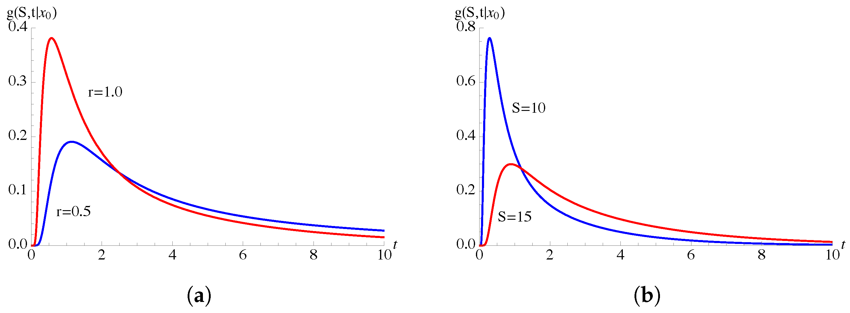
In
Figure 1, the FPT pdf
, given in (23), is plotted as function of
t for some choices of
and
r, with
.
- (b)
FPT upwards for the time-homogeneous Feller process
By virtue of (10), from (17), for
, one has
whereas for
and
, it results that:
From (24) and (25), one derives that the first passage through
S starting from
is a sure event, i.e.,
2.4. Relations between the FPT Densities for the Feller and the Wiener Processes
The FPT pdf for the time-homogeneous Feller process can be explicitly obtained for and or for and , as proved in Proposition 1 and in Proposition 2, respectively. Moreover, in these cases, there is a relationship between the FPT pdf of Feller process and the FPT pdf of the standard Wiener process.
Proposition 1. Let be a time-homogeneous Feller diffusion process, having and , with a zero-flux condition in the zero state.
If , one has: and .
If , one obtains: and .
Proof. We assume that
and
. In this case, the zero state is a regular reflecting boundary. Making use of the relations (cf. Abramowitz and Stegun [
50], p. 443, no. 10.2.14 and p. 444, no. 10.2.17)
from (19), (21), (24) and (25) with
and
, it follows that:
When
, the right-hand side of (30) identifies with the LT
of the FPT pdf
through
for a standard Wiener process originated in
. Hence, for
and
, one has
from which (27) follows. Instead, for
, the right-hand side of (30) is the LT
of the FPT pdf
through
for a standard Wiener process, starting from
, restricted to
with 0 reflecting boundary (cf., for instance, Giorno and Nobile [
3]). Then, for
and
, one obtains:
from which (28) follows. The alternative expression (29) is derived by performing the inverse LT to the second expression in (30) and by using formula 33.149, p. 190 in Spiegel et al.’s work [
51]. □
We note that by setting in (27) we obtain (23) with and .
In
Figure 2, the FPT pdf (28) is plotted as function of
t for
,
and various choices of parameters
r and
S.
Proposition 2. Let be a time-homogeneous Feller diffusion process, having and , with a zero-flux condition in the zero state.
Proof. We assume that
and
. In this case, the zero state is an entrance boundary. Making use of the relations (cf. Abramowitz and Stegun [
50], p. 443, no. 10.2.13 and p. 444, no. 10.2.17)
from (19), (24) and (25) with
and
, it follows that:
We note that when
, the right-hand side of (36) identifies with the LT
of the function
, where
is the FPT pdf through
of a standard Wiener process originated in
. Hence, for
and
, one has
that leads to (32). Instead, for
the right-hand side of (36) is the LT
of the function
, where
is the first-exit time pdf through
for a standard Wiener process, starting from
, defined in
with 0 absorbing boundary (cf., for instance, Giorno and Nobile [
3]). Then, for
and
, one has
from which (32) follows. The alternative expression (33) can be obtained by performing the inverse LT to the second expression in (36) and by using formula 33.148, p. 190 in Spiegel et al. [
51] (by changing the sign). Finally, (34) and (35) follow by taking the limit as
in (32) and (33), respectively. □
In
Figure 3, the FPT pdf (32) is plotted as function of
t for
,
and various choices of parameters
r and
S. We note that, due to the different nature of the zero state, the peaks of FPT densities of
Figure 3 are more pronounced with respect to those of
Figure 2.
2.5. Relations between the FPT Densities for the Feller and the Ornstein–Uhlenbeck Processes
For and or and , the FPT pdf of the Feller process can be related to the FPT pdf of the Ornstein–Uhlenbeck process.
Proposition 3. Let be a time-homogeneous Feller diffusion process, having and (), with a zero-flux condition in the zero state.
Proof. Let
and
. We assume that the state
is a regular reflecting boundary. Recalling that (cf. Tricomi [
48], p. 219, no. (1)):
for
from (19) one obtains (37). Furthermore, for
and
, from (21) with
and
, making use of (40), we have
Equation (41) identifies with (37) for
, being (cf. Tricomi [
48], p. 221, no. (9)):
Since (cf. Tricomi [
48], p. 234, no. 15 and p. 235, no. 18):
by setting
in (37), one obtains (38).
Instead, for , from (24) and (25), with and , one immediately obtains (39). Consequently, by setting and making use of the second expression in (13), it follows that . □
We note that, for
, the right-hand side of (37) identifies with the LT
of the FPT pdf
from
through
for the Ornstein–Uhlenbeck process with infinitesimal drift
and infinitesimal variance
. Hence, for
and
from (37) one has:
Furthermore, for
the right-hand side of (39) is the LT
of the FPT pdf
from
to
for the Ornstein–Uhlenbeck process with infinitesimal drift
and infinitesimal variance
, defined in
, with 0 reflecting boundary. Therefore, for
and
from (39), one obtains:
For
and
, relations (44) and (45) show that the FPT density of the Feller process can be also interpreted as the the FPT density of an Ornstein–Uhlenbeck process, that is known only when
. Therefore, from (44), one has:
which identifies with (23) for
and
.
Proposition 4. Let be a time-homogeneous Feller diffusion process, having and (), with a zero-flux condition in the zero state.
If , one has: If , one obtains: and .
Proof. Let
and
, so that the state
is an entrance boundary. For
, recalling that (cf. Tricomi [
48], p. 219, no. (2))
from (19), with
and
, one obtains (46). Moreover, making use of relation
and of (43), one has
so that, by setting
in (46), one obtains (47).
Instead, for from (24) and (25), with and , Equation (48) immediately follows. Finally, by setting in (48) and making use of the second expression in (13), one has . □
For
, we note that the right-hand side of (46) identifies with the LT
of
, where
is the FPT pdf from
through
for the Ornstein–Uhlenbeck process with infinitesimal drift
and infinitesimal variance
. Hence, for
and
one has:
For and , Equation (51) shows that a functional relationship between the FPT densities of the Feller and Ornstein–Uhlenbeck processes exists.
4. Asymptotic Behavior of the FPT Density for the Time-Homogeneous Feller Process
In
Section 2 and
Section 3, we analyzed the FPT problem for a time-homogeneous Feller process and we assumed that the boundary
S is constant. Nevertheless, the inclusion of a time-varying boundary
is often useful to model various aspects of the time varying behavior of dynamic systems.
Let
, with
, where
denotes the set of continuously differentiable functions on
. For a time-homogeneous diffusion process, having drift
and infinitesimal variance
, the FPT pdf
is the solution of the second-kind non-singular Volterra integral equation (cf. Buonocore [
8]):
with
if
and
if
, and where
The knowledge of the transition pdf
of the considered diffusion process allows the formulation of effective numerical procedures to obtain
via (57) (cf., for instance, Buonocore et al. [
8], Di Nardo et al. [
10]).
For the Feller process, having
and
, with a zero-flux condition in the zero state, recalling (5) and (6), for
from (58), one obtains:
where the relation (cf. Gradshteyn and Ryzhik [
47], p. 928 no. 8.486.4)
has been used.
Let . We focus our analysis on the asymptotic behavior of the FPT pdf for the Feller diffusion process, with , and , by considering separately two cases: is an asymptotically constant boundary and is an asymptotically periodic boundary.
4.1. Asymptotically Constant Boundary
We consider the FPT problem for the Feller process through the asymptotically constant boundary
with
, where
is a bounded function that does not depend on
S, such that
Since
, the function
approaches a constant value as
. Making use of (60), for
, one has:
where (9) has been used. From (57), for
and for large times the FPT density exhibits an exponential behavior (cf. Nobile et al. [
12]). Specifically, for
and
, one has:
The goodness of the exponential approximation increases as the boundary progressively moves away from the starting point.
We now assume that the boundary
is constant, i.e.,
. By virtue of (53) for
, with
and
defined in (4), and recalling (63), for
and
one has
implying that for
the FPT mean can be approximated by
for large values of
S. Furthermore, by virtue of (64), for
and
, one obtains:
In
Table 2, the FPT moments
and their exponential approximations
, with
, are listed for increasing values of the boundary
, showing a good degree of precision in the approximations. We emphasize that the exponential approximation of the FPT density (64) provides the growth trend of the FPT moments (65) for large constant boundaries
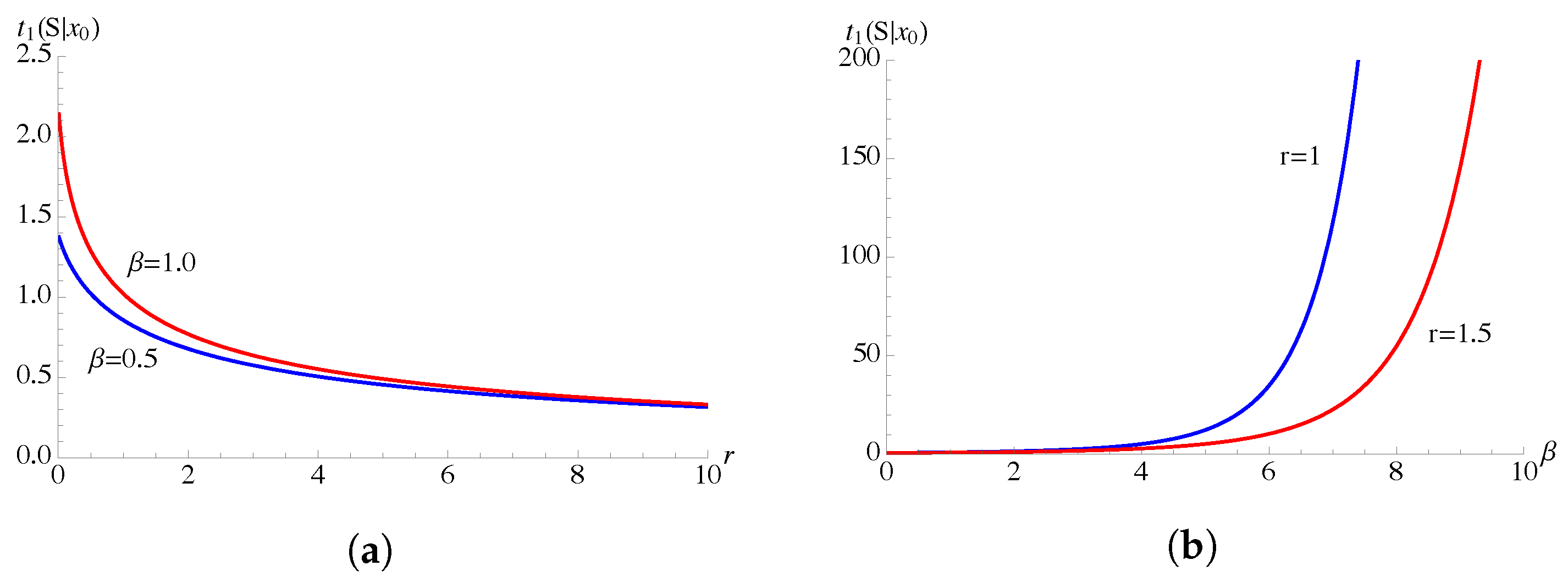
S. Moreover, the goodness of the approximation depends on the parameters of the process that determine the exact shape of the FPT pdf.
4.2. Asymptotically Periodic Boundary
We consider the FPT problem for the Feller process through an asymptotically periodic boundary
, with
, where
is a bounded function, that does not depend on
S, such that
with
being a periodic function of period
satisfying the condition:
Since
, the function
approaches a periodic function as
. Indeed, making use of (60) and recalling (9), for
, one obtains:
By virtue of (57), for
and for large times, the FPT density shows a non-homogeneous exponential behavior. Specifically, for
and
, one has:
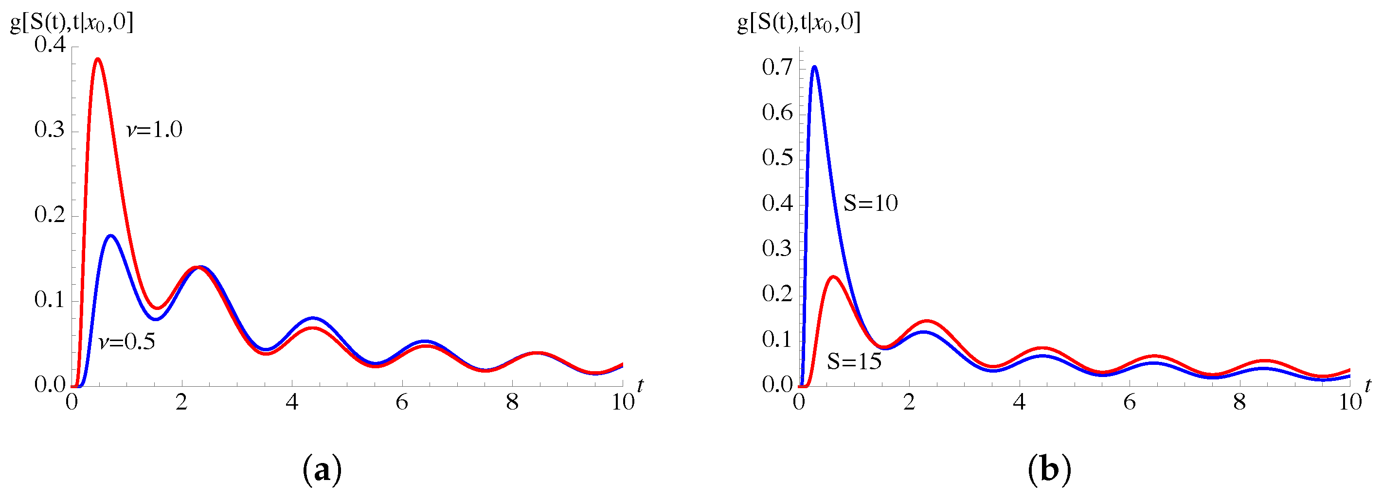
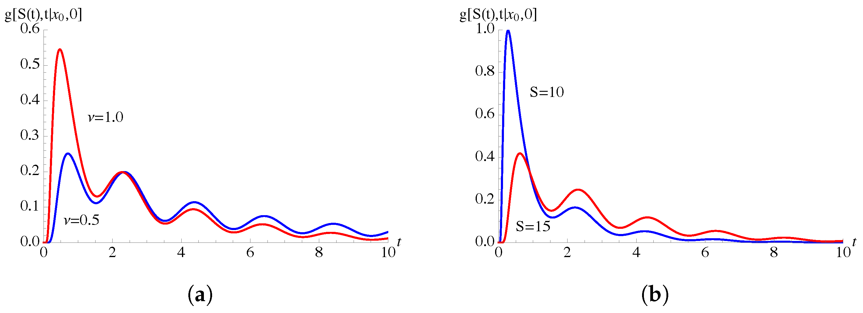
Hence, for , the FPT pdf of the Feller process through an asymptotically periodic boundary exhibits damped oscillations taking the form of a sequence of periodically spaced peaks whose amplitudes exponentially decrease.
6. Asymptotic Behavior of the FPT Density for a Time-Inhomogeneous Feller-Type Process
In the following proposition, we prove that the FPT density of the process (69), with a zero-flux condition in the zero state, is a solution of a second-kind non-singular Volterra integral equation.
Proposition 8. Let , with . For the time-inhomogeneous Feller-type diffusion process (69), with , and , the FPT pdf is a solution of the integral Equation (57) with if and if , where Proof. The FPT pdf
of the process
, with infinitesimal drift
and infinitesimal variance
, with a zero-flux condition in the zero state, is a solution of the following integral equation
where, due to (59) with
and
, one has:
Multiplying both-sides of Equation (91) by
, performing the transformation
in the integral and recalling (79), we obtain the integral Equation (57) with
Then, (90) follows from (93), making use of (74) and (92). □
Let
. We focus on the asymptotic behavior of the FPT pdf of the Feller-type diffusion process (69), with a zero-flux condition in the zero state, through the asymptotically constant boundary (61), with
, where
is a bounded function, that does not depend on
S, such that (62) holds. We assume that
so that the process allows a steady-state density. Under such assumptions, from (90), one has:
Finally, by virtue of (57), for
and for long periods, the FPT density through the asymptotically constant boundary (61) of the time-inhomogeneous Feller-type process (69) exhibits the following exponential behavior:
7. Conclusions
In this paper, we have considered the first-passage time problem for a Feller-type diffusion process, having infinitesimal drift
and infinitesimal variance
, defined in
, with
,
,
continuous functions. In
Section 2, for the time-homogeneous process, we have determined the Laplace transform of the downwards and upwards FPT densities. In Propositions 1 and 2, some connections between the FPT densities for the Feller and the Wiener processes (
) have been discussed, whereas in Propositions 3 and 4 we have analyzed some relations between the FPT densities for Feller and Ornstein–Uhlenbeck processes (
). Furthermore, in
Section 3, the FPT moments have been investigated by using the Siegert formula. In
Section 4, for
, the asymptotic behavior of the FPT density through a time-dependent boundary has been discussed for an asymptotically constant boundary and for an asymptotically periodic boundary. Furthermore, the first three moments of FPT density through a constant boundary have been compared with the corresponding asymptotic approximations.
Section 5 is dedicated to a time inhomogeneous Feller-type diffusion process with
, for
. In Propositions 6 and 7, the FPT density has been obtained for an exponential time-varying boundary. The FPT densities have been plotted for periodic noise, showing the presence of damped oscillations having the same periodicity as the noise intensity. In
Section 6, a second-kind Volterra integral equation was derived for the FPT density of a time-inhomogeneous Feller-type process through a general time-dependent boundary. Finally, such an equation has been used to derive the asymptotic exponential trend of the FPT pdf through an asymptotically constant boundary.
Analytical, asymptotic and computational methods for the evaluation of FPT densities through time-varying boundaries for more general time-inhomogeneous diffusion processes will be the object of future research focused also on contexts of statistical inference.


