Multi-Objective Pharmaceutical Portfolio Optimization under Uncertainty of Cost and Return

Abstract

This paper presents the study of multi-objective optimization of a pharmaceutical portfolio when both cost and return values are uncertain. Decision makers in the pharmaceutical industry encounter several challenges in deciding the optimal selection of drug projects for their portfolio since they have to consider several key aspects such as a long product-development process split into multiple phases, high cost and low probability of success. Additionally, the optimization often involves more than a single objective (goal) with a non-deterministic nature. The aim of the study is to develop a stochastic multi-objective approach in the frame of chance-constrained goal programming. The application of the results of this study allows pharmaceutical decision makers to handle two goals simultaneously, where one objective is to achieve a target return and another is to keep the cost within a finite annual budget. Finally, the numerical results for portfolio optimization are presented and discussed.

1. Introduction

A drug development project is a long-term multi-phase process where investments are generally decided at a decision point prior to each phase. The cost of development increases as the project progresses through the phases. Most projects are terminated due to technical, regulatory or commercial issues, leaving only a very small number of drugs that reach the market. When a project fails, the cost of development has been imposed on the pharmaceutical company without any opportunity of a refund. The most complex and vital challenge in the decision-making process of pharmaceutical companies is identifying the optimal selection of projects for the drug development portfolio, including allocating finite budgets to long-term investment opportunities [1]. 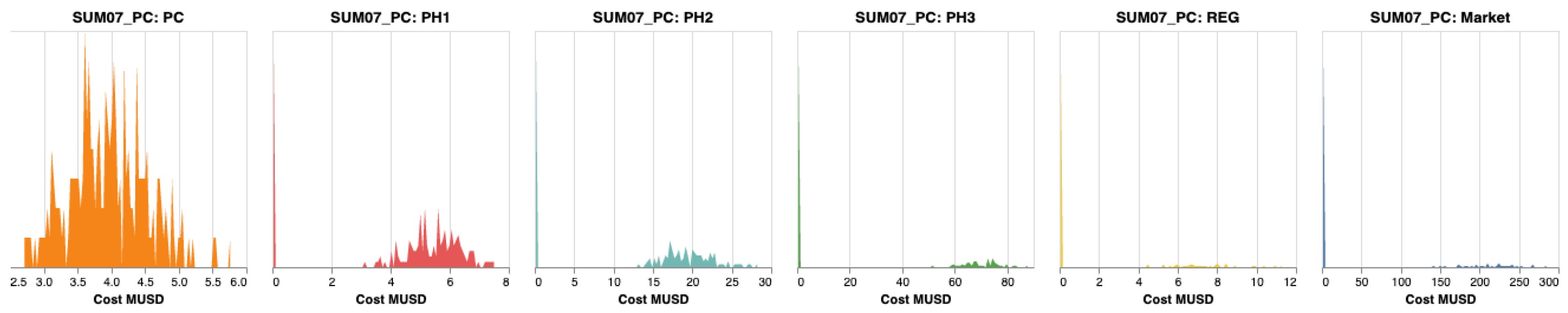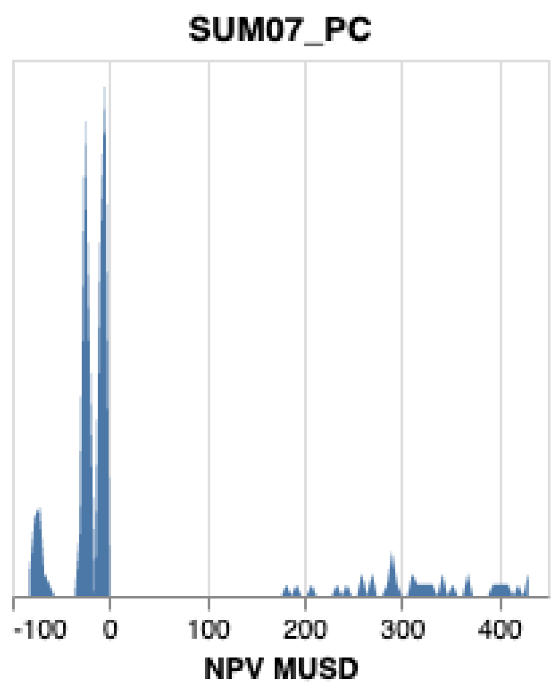The challenges include taking into account the multiple phases of the drug project, uncertainty in the cost of each phase, the uncertainty of returns only in part due to a high probability of failure [2,3]. The multi-modal probability distributions describing the uncertainties do not make it easier, see Figure A1 and Figure A2 in Appendix A. In addition, there are often dependencies that affect the outcome of projects. For example, one project may cannibalize sales from another or several projects may build on a common platform, thereby sharing risks. Additionally, real-world portfolios are dynamic in nature and change over time. Projects are terminated and new projects are included in the portfolio. These may come from the internal research organization and start in the earliest phase or be added through in-licensing or acquisition into any phase.

Traditional methods for portfolio decision making often focus on different ranking algorithms, which can be improved upon by the use of mathematical optimization [4]. For an optimal project selection, mathematical modeling and optimization techniques can improve budget allocation to the right projects to achieve a maximal performance of the portfolio. However, the uncertainty inherent in any pharmaceutical project means that applying deterministic optimization cannot lead to a correct decision for the pharmaceutical portfolio. To increase the effectiveness of the project selection process, it is necessary to consider the uncertain nature of time, cost and revenue, as well as the probability of failure for each of the projects together with the limitations of the development budget. To that end, stochastic programming is a powerful approach for capturing and handling uncertainty in projects since it is based on random data. Moreover, portfolio optimization most often involves optimization of several goals simultaneously with sometimes conflicting objectives. Employing a single objective optimization approach leads to inaccurate mathematical modeling of portfolio optimization. The result derived from such an “inaccurate model” is not reliable and can mislead decision makers [5].

The aim of this study is to develop a pharmaceutical portfolio optimization tool based on a stochastic multi-objective optimization algorithm, which is not only scientifically reliable but also simple to implement as an easy-to-use working tool in the pharmaceutical industry. This tool lets decision makers handle more than one objective under uncertainty and to decide whether to give more weight to reaching the maximum return or to staying within a finite annual budget. Hence, it will be possible to increase the portfolio value with respect to multi-performance goals and imposing constraints. The paper is organized as follows. In the next section, the background of mathematical optimization is discussed and then the mathematical model for a multi-objective optimization problem with data uncertainty and an approach for solving it are proposed. In Section 3, we describe our pharmaceutical portfolio optimization problem and its solution. We discuss the numerical results in Section 4 and Section 5 is the conclusion of the paper.

2. Goal-Programming with Data Uncertainty

Multi-objective optimization (also known as multi-objective programming) has been developed to solve optimization problems when it is necessary to optimize several objectives that may be in conflict with each other. Multi-objective optimization has been widely used in many real-world decision making problems in different fields such as energy, transportation and portfolio management. Several studies have been focused on proposing approaches to solving optimization problems with multiple objectives (see [6,7,8]). In 1961, Charnes and Cooper [9] presented a goal programming approach for handling multi-criteria decision analysis, which enables decision makers to insert more than one objective. Goal programming is a class of multi-objective optimization, which solves optimization problems with multiple objective functions that may be contrary to each other within a decision-making horizon. In optimizing a multi-objective problem, you would ideally find an optimal solution in which every objective is optimized. This is often not possible in reality. Using goal programming, decision makers specify the target value for each objective that is aimed for. If an optimal solution cannot be found that reaches all of the target values, then an optimal solution is found such that it minimizes deviation from the target values.

The general mathematical model of weighted goal programming is constructed as follows.

$$\begin{array}{ccc}\hfill & \mathrm{minimize}\hfill & \hfill w_1^{+}{d}_1^{+}+w_2^{-}{d}_2^{-}\\ \\ \hfill & \mathrm{subject}\mathrm{to}:\hfill \\ \hfill & \mathrm{Goal}\mathrm{constraint}1:\hfill & \hfill \sum _{i=1}^n{a}_i{x}_i-d_1^{+}\le A,\\ \hfill & \mathrm{Goal}\mathrm{constraint}2:\hfill & \hfill \sum _{i=1}^n{b}_i{x}_i+d_2^{-}\ge B,\\ \hfill & \mathrm{System}\mathrm{constraints}:\hfill & \hfill \sum _{i=1}^n{e}_{ij}{x}_i\left[\begin{array}{c}\le \\ =\\ \ge \end{array}\right]E_j,j=1,\dots ,m\\ \\ \hfill & \hfill & \hfill d_1^{+},d_2^{-},x_i\ge 0i=1,\dots ,n\end{array}$$

(1)

In this model, $x_i$ are decision variables and $d_1^{+}$ and $d_2^{-}$ are the positive and negative deviations of goal constraints 1 and 2, respectively. The weights of the deviations, as defined by decision makers, are represented by $w_1^{+}$ and $w_2^{-}$. Coefficients of decision variables are denoted by $a_i$, $b_i$, $e_{ij}$; A, B are target values of goal constraints 1 and 2, respectively; and $E_j$ is the right-hand-side of the system constraint.

Employing multi-objective optimization to solve a single optimization problem when problems have more than one objective can improve the efficiency of the solution. However, it is not enough for an accurate solution to many real-world problems. In reality, most often, decision makers need to take into account the uncertainty of coefficients for the solution to be adequate. Hence, the mathematical modeling of optimization problems must not only contain multiple objectives but also include the uncertainty of coefficients. Stochastic programming is an effective approach for solving optimization problems under uncertainty of data. One approach of stochastic programming is chance constrained programming [10], which has been widely employed to handle the uncertainty of constraint coefficients when they are random variables.

With this method, decision makers can allow violation of specific constraints, which must be satisfied within defined confidence levels. These constraints are named chance constraints. The mathematical model of chance constrained goal programming can be presented as follows.

$$\begin{array}{ccc}\hfill & \mathrm{minimize}\hfill & \hfill w_1^{+}{d}_1^{+}+w_2^{-}{d}_2^{-}\\ \\ \hfill & \mathrm{subject}\mathrm{to}:\hfill \\ \hfill & \mathrm{Chance}\mathrm{goal}\mathrm{constraint}1:\hfill & \hfill Prob\left\{\sum _{i=1}^n{a}_i{x}_i-d_1^{+}\le A\right\}\ge {\beta }_1,\\ \hfill & \mathrm{Chance}\mathrm{goal}\mathrm{constraint}2:\hfill & \hfill Prob\left\{\sum _{i=1}^n{b}_i{x}_i+d_2^{-}\ge B\right\}\ge {\beta }_2,\\ \hfill & \mathrm{System}\mathrm{Constraints}:\hfill & \hfill \sum _{i=1}^n{e}_{ij}{x}_i\left[\begin{array}{c}\le \\ =\\ \ge \end{array}\right]E_j,j=1,\dots ,m\\ \\ \hfill & \hfill & \hfill d_1^{+},d_2^{-},x_i\ge 0i=1,\dots ,n,\end{array}$$

(2)

where $a_i$, $b_i$ are coefficients of decision variables under uncertainty and ${\beta }_1,{\beta }_2\in (0,1)$ are confidence levels defined by decision makers. A chance constraint can be formulated as an individual chance constraint or a joint chance constraint (see [11,12]).

Chance constrained programming has received lots of attention for handling the uncertainty of data, but several challenges exist for solving the model of a chance constrained programming problem in real applications. Different approaches that depend on the probability distributions of uncertain data have been presented for chance constrained optimization. These approaches have been constructed for random variables with a known, single-modal distribution, where the chance constraint can be converted into an equivalent deterministic constraint using a probability density function.

Recently, Farid et al. [13] presented an approach for solving pharmaceutical portfolio optimization, where the coefficients of decision variables in constraints make up a finite set of random variables with unknown distributions. They employed chance constraint programming to model a portfolio optimization problem and then found the optimal solution for the portfolio by using binary control variables $z_k,$$k=1,2,..,N$ and “big M” coefficients. In their portfolio optimization problem, they considered coefficients of the objective function as constant values. One limitation of the Farid et al. approach is that uncertainty is only considered in the constraints whereas it would be beneficial to also consider uncertainty in the objective function. By rephrasing the uncertain objective function as a chance constraint and defining minimization of deviation as the new objective function, we can formulate a new, extended model, named MICCG (Big-M, Integer, Chance Constrained Goal programming) as

$$\begin{array}{ccc}\hfill & \mathrm{minimize}\hfill & \hfill w_1^{+}{d}_1^{+}+w_2^{-}{d}_2^{-}\\ \\ \hfill & \mathrm{subject}\mathrm{to}:\hfill \\ \hfill & \mathrm{Big}\mathrm{M}\mathrm{chance}\mathrm{goal}\mathrm{constraint}1:\hfill & \hfill \sum _{i=1}^n{a}_i{x}_i-d_1^{+}-M{z}_k\le A,k=1,\dots ,N.,\\ \hfill & \hfill & \hfill \sum _{k=1}^N{z}_k{\pi }_k\le 1-{\beta }_1,\\ \hfill & \mathrm{Big}\mathrm{M}\mathrm{chance}\mathrm{goal}\mathrm{constraint}2:\hfill & \hfill \sum _{i=1}^n{b}_i{x}_i+d_2^{-}+M{q}_k\ge B,k=1,\dots ,N.,\\ \hfill & \hfill & \hfill \sum _{k=1}^N{q}_k{p}_k\le 1-{\beta }_2,\\ \hfill & \mathrm{System}\mathrm{Constraints}:\hfill & \hfill \sum _{i=1}^n{e}_{ij}{x}_i\left[\begin{array}{c}\le \\ =\\ \ge \end{array}\right]E_j,j=1,\dots ,m,\\ \\ \hfill & \hfill & \hfill d_1^{+},d_2^{-},x_i\ge 0,i=1,\dots ,n\\ \hfill & \hfill & \hfill z_k,q_k\in \{0,1\}\end{array}$$

(3)

where $M\ge 0$ is a large constant and ${\beta }_1,{\beta }_2\in (0,1)$. There are N scenarios for each coefficient of the goal constraints and the probabilities of each scenario in the goal big M chance constraints 1 and 2 are ${\pi }_k$ and $p_k$$(k=1,\dots ,N)$, respectively. When the binary control variables, $z_k$ and $q_k$ are equal to zero, it means that the related constraints have to be strictly satisfied; otherwise, violation is permitted up to the accepted risk level (see [9,10,14]). In the case where the decision variables in the model (3) are also binary, then an integer programming solver can solve it.

3. Pharmaceutical Portfolio Optimization under Uncertainty of Cost and Return

The drug development process running through multiple phases has a low probability of success, a long and uncertain duration, as well as uncertainty in cost and return. These uncertainties make pharmaceutical portfolio optimization extremely challenging. Hence, decision makers face difficulties in allocating limited budgets to the projects in order to achieve their goals. In this study, our aim is to present an approach that is able to deal with uncertainty of data in the return and cost of projects when there is more than one goal. The goals here are to find an optimal project selection that fulfills an annual budget limitation and, at the same time, to reach the return target. Our pharmaceutical portfolio optimization problem is thus described. A drug development project is a multi-phase process, and the cost of running a phase is distributed by year for the duration of the phase. If a project fails in a phase, the project is terminated at the end of the phase and the cost of the subsequent phases is zero. If the product fails to reach the market, the revenue is zero. For the portfolio, there is a target for the combined return and a yearly budget limit. We denote the cost of project i in year j as $c_{ij}$ and the return of each project by $r_i$.

Using Monte Carlo simulation, we create N scenarios in which $c_{ij}$ and $r_i$ are random variables and the probability of each scenario is ${\displaystyle \frac{1}{N}}$. The probability distributions of the random variables $c_{ij}$ and $r_i$ are multi-modal distributions; see Figure A1 and Figure A2. Generally, pharmaceutical portfolio optimization is multi-objective with objectives (goals) consisting of decreasing cost and increasing return with binary decision variables. The weight of each objective is determined by decision makers. In goal programming, each objective is described as one constraint and since in our problem cost and return are under uncertainty, we describe each of our objectives in the frame of chance constraints as follows.

• The total costs are not more than the annual budget at least within the defined confidence level.
• The total return is not less than target return at least within the defined confidence level.

In our pharmaceutical optimization problem, we have more than one goal and our data are under uncertainty, so we accept the proposed approach in (3) for solving our problem. Expressing our mathematical model in the MICCG (3) frame for the pharmaceutical portfolio optimization problem, we have the following:

$$\begin{array}{ccc}\hfill & \mathrm{minimize}\hfill & \hfill \sum _{j=1}^T{w}_1^{+}{d}_{1j}^{+}+w_2^{-}{d}_2^{-}\\ \\ \hfill & \mathrm{subject}\mathrm{to}:\hfill \\ \hfill & \mathrm{Budget}\mathrm{goal}:\hfill & \hfill \sum _{i=1}^n{c}_{ij}{x}_i-d_{1j}^{+}-M{z}_{kj}\le B_j,\\ \hfill & \hfill & \hfill {\displaystyle \frac{1}{N}}\sum _{k=1}^N{z}_{kj}\le 1-{\beta }_j,\\ \hfill & \mathrm{Return}\mathrm{goal}:\hfill & \hfill \sum _{i=1}^n{r}_i{x}_i+d_2^{-}+M{q}_k\ge R,\\ \hfill & \hfill & \hfill {\displaystyle \frac{1}{N}}\sum _{k=1}^N{q}_k\le 1-\alpha ,\\ \hfill & \hfill & \hfill d_{1j}^{+},d_2^{-}\ge 0,x_i,z_{kj},q_k\in \{0,1\}\\ \hfill & \hfill & \hfill i=1,\dots ,n,j=1,\dots ,T,k=1,\dots ,N.\end{array}$$

(4)

where decision variables $x_i\in \{0,1\}$, $i=1,\dots ,n$ are binary. If $x_i=1$, then project i is chosen to be included in the portfolio. The minimum desired confidence levels for the budget and return constraints are $\beta ,\alpha \in (0,1)$, respectively. Lastly, M is a sufficiently large number. When $z_{kj}=1,$ the budget constraint related to the year j may be violated. This may happen at most in $N(1-\beta )$ scenarios. Otherwise, $z_{kj}=0$ shows that the budget constraint in year j must be satisfied. Moreover, when $q_k=1$, the return constraint may be violated up to the maximum risk $1-\alpha$. Otherwise, $q_k=0$ means that the target constraint has to be satisfied. The budget limitation in year j, $j=1,\dots ,T$ is $B_j$ and R is the target value for return. The non-negative weights $w_1^{+},w_2^{-}$ are related to each goal and defined by decision makers. They show the importance of each goal for the decision makers. If the deviation variables $d_{1j}^{+},d_2^{-}$ are all equal to zero, the goals do not conflict and decision makers can reach both goals simultaneously without the requirement of deviation.

4. Numerical Results for Pharmaceutical Project Portfolio Selection

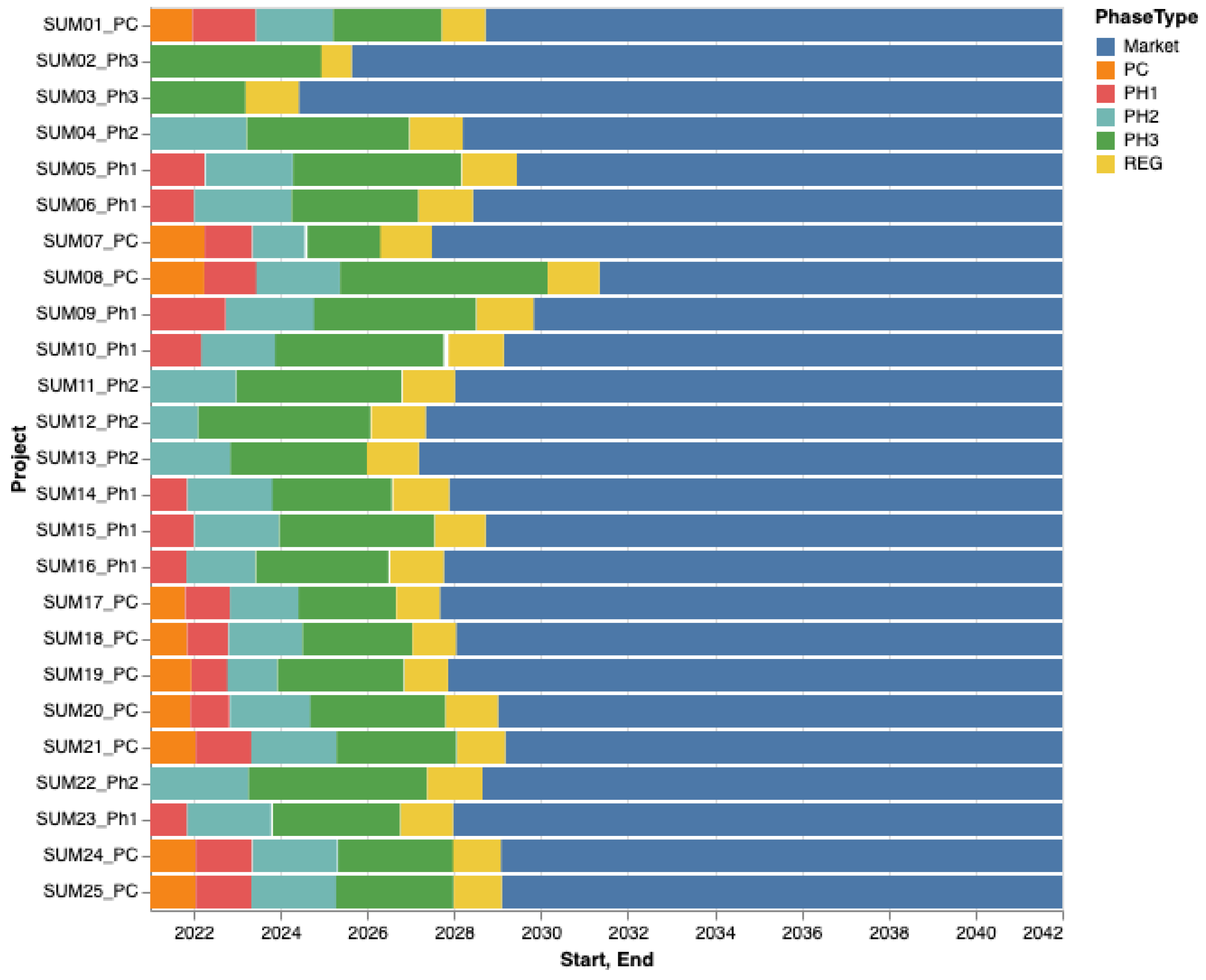
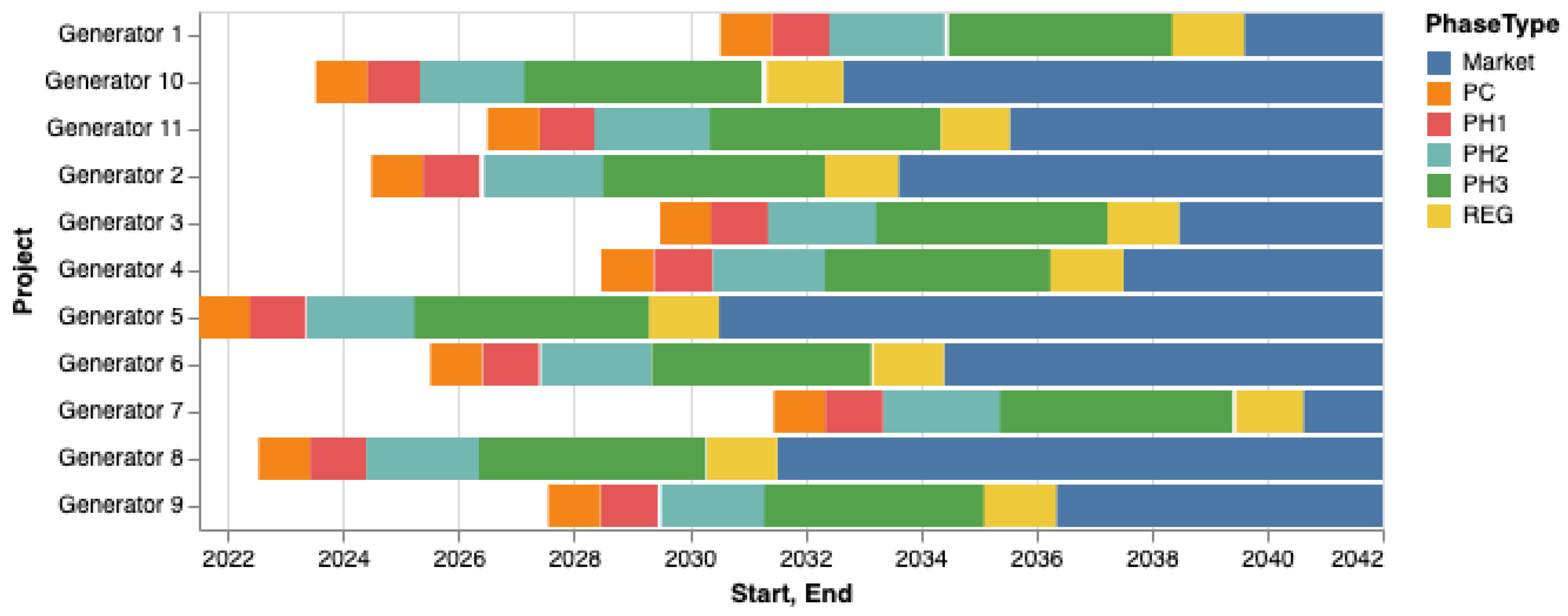
In this section, we present the numerical results for a sample pharmaceutical portfolio to show how our proposed approach (4) works. The algorithm was written in Python 3. We employed CPLEX for solving our multi-objective linear programming problem with binary decision variables. The experiments were run on an Intel(R) Core i9 CPU, 2.3 GHz and 16 GB of RAM. The sample portfolio was constructed by experienced portfolio analysts to be similar to the portfolio of a medium-sized pharma company. The portfolio consists of 36 projects in various phases. There are 25 ongoing projects, of which ten are in the preclinical phase (PC), eight are in phase 1 (PH1), five are in phase 2 (PH2) and two projects are in phase 3 (PH3). The portfolio will be dynamically extended with one project per year for 11 years starting in the preclinical phase. The portfolio model includes 200 random variables. The planning horizon of portfolio, T, equals 20 years. Figure A3 and Figure A4 show the timelines of the projects in our portfolio. Ongoing projects are numbered and include the current phase in their name and added projects are named “Generator N”.

The problem for decision makers is to decide how to allocate their limited annual budget such that the portfolio returns not be less than a specified target. In this numerical analysis, we consider Net Present Value (NPV) as our measure of return. We defined three scenarios. For all three, we set the confidence levels for return and budget ($\alpha$ and ${\beta }_j$) to 75% and 80% respectively. Additionally, the budget is set to 150 MUSD per year. Other inputs to the model (4) for the respective scenarios are listed in the

Table 1. The optimal project selection for Scenario 1.

Scenario 1—input
Weights	$w_1^{+}$ (budget)	1
	$w_2^{-}$ (return)	1
Confidence levels	${\beta }_j$ (budget)	$80\%$ (each year)
	$\alpha$ (return)	$75\%$
Return target (NPV)	R	3500 MUSD
Allocated budget	$B_j$	150 MUSD per year
Scenario 1—output
Budget deviation $\left(d_1^{+}\right)$	$[0,0,0,0,0,0,0,0,0,0,0,0,0,0,0,0,0,0,0,0]$
Budget confidence level (${\beta }_j$)	[$100\%$,$98\%$,$83\%$,$93\%$,$98\%$,$100\%$,$100\%$,$100\%$,$100\%$,$100\%$,
	$100\%$,$100\%$,$100\%$,$100\%$,$100\%$,$100\%$,$100\%$,$100\%$,$100\%$,$100\%$]
Return target deviation $\left(d_2^{-}\right)$	0
Return target	$75\%$
Confidence level ($\alpha$)
Selected projects	’SUM01-PC’, ’SUM02-Ph3’, ’SUM03-Ph3’, ’SUM04-Ph2’,
	’SUM06-Ph1’, ’SUM09-Ph1’, ’SUM10-Ph1’, ’SUM11-Ph2’,
	’SUM13-Ph2’, ’SUM15-Ph1’, ’SUM16-Ph1’, ’SUM22-Ph2’,
	’SUM23-Ph1’,

,

Table 2. The optimal project selection for Scenario 2.

Scenario 2—input
Weights	$w_1^{+}$ (budget)	1
	$w_2^{-}$ (return)	1
Confidence levels	${\beta }_j$ (budget)	$80\%$ (each year)
	$\alpha$ (return)	$75\%$
Return target (NPV)	R	4500 MUSD
Allocated budget	$B_j$	150 MUSD per year
Scenario 2—output
Budget deviation$\left(d_1^{+}\right)$	$[0,7.9,42.7,25.7,3.3,0,0,0,0,0,0,0,0,0,0,0,0,0,0,0]$
Budget confidence level (${\beta }_j$)	[$99\%$,$80\%$,$80\%$,$80\%$,$80\%$,$86\%$,$95\%$,$100\%$,$100\%$,$100\%$,
	$100\%$,$100\%$,$100\%$,$100\%$,$100\%$,$100\%$,$100\%$,$100\%$,$100\%$,$100\%$]
Return target deviation $\left(d_2^{-}\right)$	351.6
Return target	$75\%$
Confidence level ($\alpha$)
Selected projects	’SUM01-PC’, ’SUM02-Ph3’, ’SUM03-Ph3’, ’SUM04-Ph2’,
	’SUM05-Ph1’, ’SUM06-Ph1’, ’SUM08-PC’, ’SUM09-Ph1’,
	’SUM10-Ph1’, ’SUM11-Ph2’, ’SUM14-Ph1’, ’SUM15-Ph1’,
	’SUM16-Ph1’, ’SUM22-Ph2’, ’SUM23-Ph1’, ’SUM24-Ph1’,
	’SUM25-Ph1’,’Generator 8’

and

Table 3. The optimal project selection for Scenario 3.

Scenario 3—input
Weights	$w_1^{+}$ (budget)	4
	$w_2^{-}$ (return)	1
Confidence levels	${\beta }_j$ (budget)	$80\%$ (each year)
	$\alpha$ (return)	$75\%$
Return target (NPV)	R	4500 MUSD
Allocated budget	$B_j$	150 MUSD per year
Scenario 3—output
Budget deviation$\left(d_1^{+}\right)$	$[0,5.4,38,18.3,0.80,0,0,0,0,0,0,0,0,0,0,0,0,0,0,0]$
Budget confidence level (${\beta }_j$)	[$99\%$,$80\%$,$80\%$,$80\%$,$80\%$,$87\%$,$96\%$,$100\%$,$100\%$,$100\%$,
	$100\%$,$100\%$,$100\%$,$100\%$,$100\%$,$100\%$,$100\%$,$100\%$,$100\%$,$100\%$]
Return target deviation $\left(d_2^{-}\right)$	415
Return target	$75\%$
Confidence level ($\alpha$)
Selected projects	’SUM01-PC’, ’SUM02-Ph3’, ’SUM03-Ph3’, ’SUM04-Ph2’,
	’SUM05-Ph1’, ’SUM06-Ph1’, ’SUM08-PC’, ’SUM09-Ph1’,
	’SUM10-Ph1’, ’SUM11-Ph2’, ’SUM14-Ph1’, ’SUM15-Ph1’,
	’SUM16-Ph1’, ’SUM22-Ph2’, ’SUM23-Ph1’,’SUM24-Ph1’,
	’SUM25-Ph1’

.

For Scenario 1, the return target is set to 3500 MUSD and the weights for budget ($w_1^{+}$) and return ($w_2^{-}$) are both 1.

In Table 1, 13 ongoing projects are selected into the portfolio. The components of the budget vector, i.e., the annual budget deviations, are all zero, which shows that the optimal selection of projects can be funded within the budget constraints. In addition, the return deviation is also zero, which shows that the NPV goal can be fulfilled. Hence, both goals can simultaneously be satisfied and there is no conflict between the budget goal and the NPV goal.

In Scenario 2, we change the return target to 4500 MUSD. The output in Table 2 shows that the revenue target cannot be achieved with the current budget constraints. In this case, the algorithm selects projects to minimize the deviation from the budget and return target. The new budget increases in years 2, 3, 4 and 5 by 7.9, 42.7, 25.7 and 3.3 MUSD, respectively, and the new return target is 4148.4 MUSD. With these new values, there is at least a 75% chance of achieving the return target and a 80% chance of keeping within the budget.

In the last scenario, we have a situation where the budget is more constrained. Therefore, we increase the weight for budget deviations to 4, thereby increasing the priority of keeping within budget. Practically, it means that budget deviations “cost” four times as much as a corresponding deviation from the return target.

The resulting selection of projects has budget deviations 5.4, 38.0, 18.3 and 0.80 in years 2, 3, 4 and 5, respectively, but a larger deviation from the return target. In this scenario, the return target should be decreased to 4085 MUSD. Again, these changes result in a situation where there is a 80% chance of keeping within the budget and a 75% chance of achieving the return target.

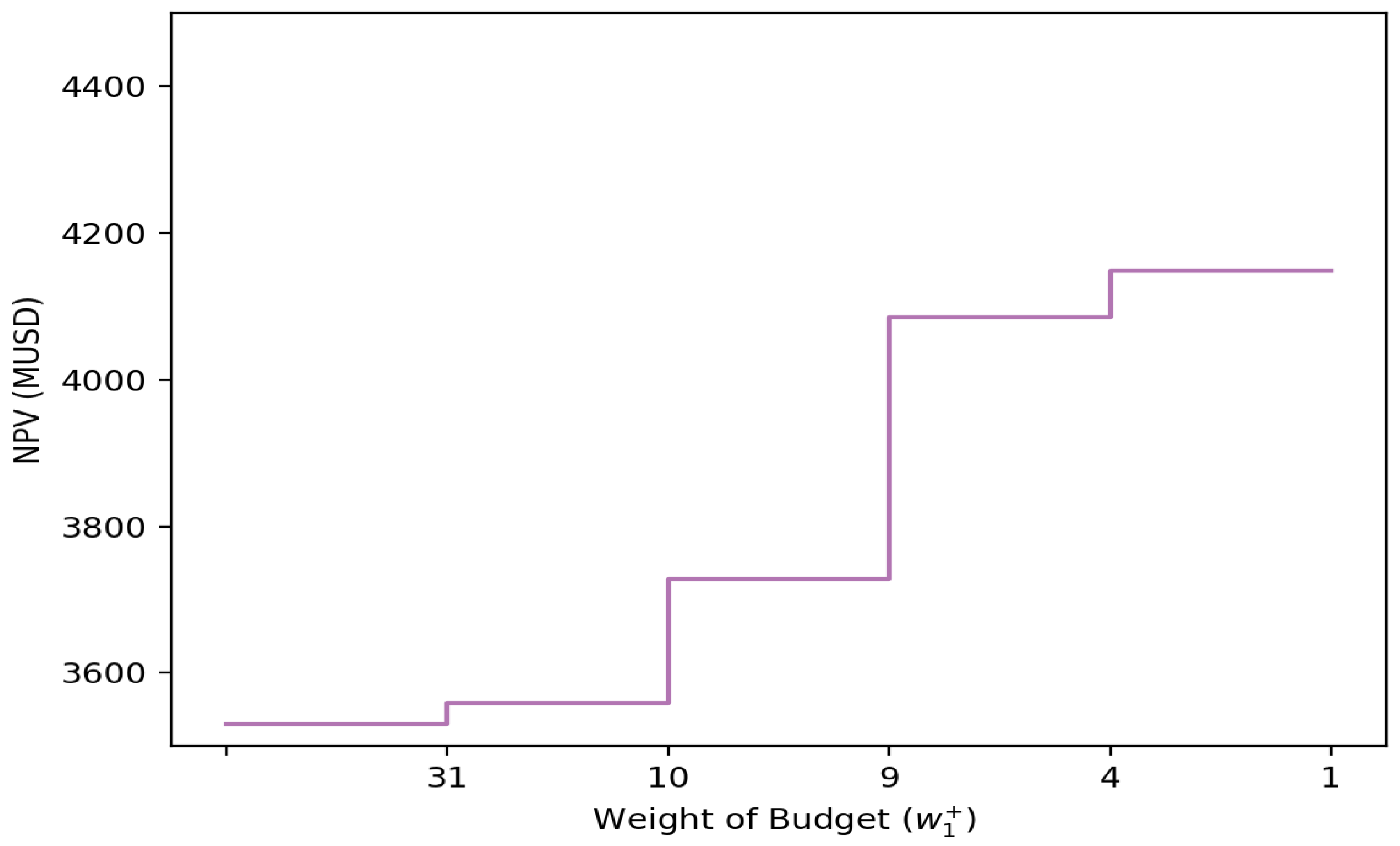
Since the solution to the optimization problem is a discrete selection of projects, it stands to reason that not every change in inputs results in a change in output. To illustrate this, we change the weight of the budget in the object function in (4) in unit steps. The higher weight of the budget constraints reduces the deviation from the target budget but increases the deviation from the return target. Using the inputs for scenario 2, the selection of projects and the return deviation changes at weights $w_1^{+}=\{1,4,9,10,31\}$. Figure 1 shows the probable target return versus the weight of the budget constraints, and

Table 4. Weight of budget vs. budget deviation.

${\mathit{w}}_1^{+}$	Budget Deviation	Altered Target Return (NPV)
1	$[0,7.9,42.7,25.7,3.3,0,0,0,0,0,0,0,0,0,0,0,0,0,0,0]$	4148.4
4	$[0,5.4,38,18.3,0.80,0,0,0,0,0,0,0,0,0,0,0,0,0,0,0]$	4085
9	$[0,0.1,19.1,0,0,0,0,0,0,0,0,0,0,0,0,0,0,0,0,0]$	3727.7
10	$[0,0,1,0,0,0,0,0,0,0,0,0,0,0,0,0,0,0,0,0]$	3558.8
31	$[0,0,0,0,0,0,0,0,0,0,0,0,0,0,0,0,0,0,0,0]$	3530

also shows the expected deviation from the budget. For weights $w_1^{+}\ge 31$, the budget deviation is 0 so nothing changes by increasing it further.

5. Conclusions

As mentioned in the Introduction, pharmaceutical R&D is full of uncertainty. Therefore, decision support methods should include uncertainty of input parameters as well as qualifiers for the outputs. In this paper, we describe the project selection process for pharma R&D portfolios as a multi-objective optimization problem where data are uncertain with unknown probability. The proposed method allows a decision maker to explicitly enter their level of risk acceptance in terms of confidence levels and weightings. The underlying portfolio model can also include all relevant aspects of the projects, including but not limited to common risks and cannibalization of sales. The result of the optimization is a selection of projects that maximizes the return of the portfolio while keeping the budget within an acceptable range. This result has the advantage of contributing a holistic and quantitative perspective to a decision-making process that is often predominantly qualitative. Further research will look into questions of the stability of the optimal solution given small changes of the budget and/or the return target. We also propose to investigate how this algorithm may be used in a real setting where multiple decisions are made over time.