
Flow towards a Stagnation Region of a Curved Surface in a Hybrid Nanofluid with Buoyancy Effects


Abstract
1. Introduction
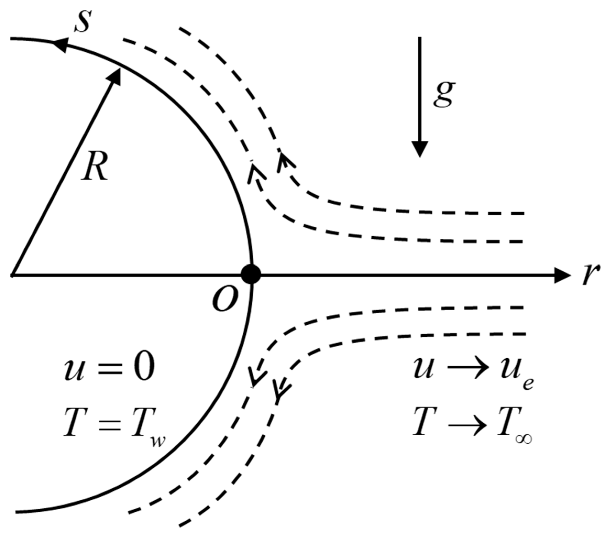
2. Basic Equations
3. Similarity Transformations
4. Stability Analysis
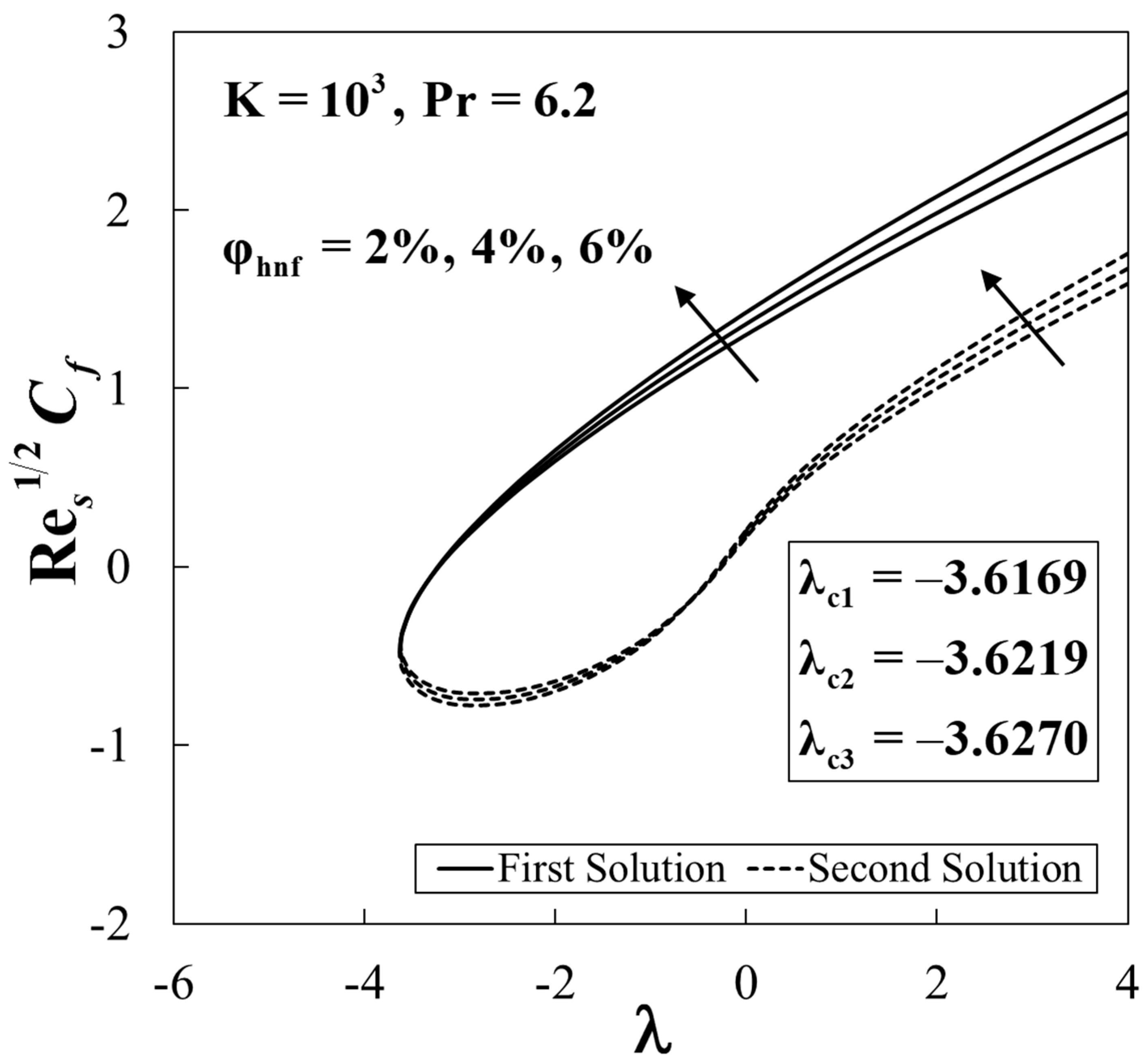
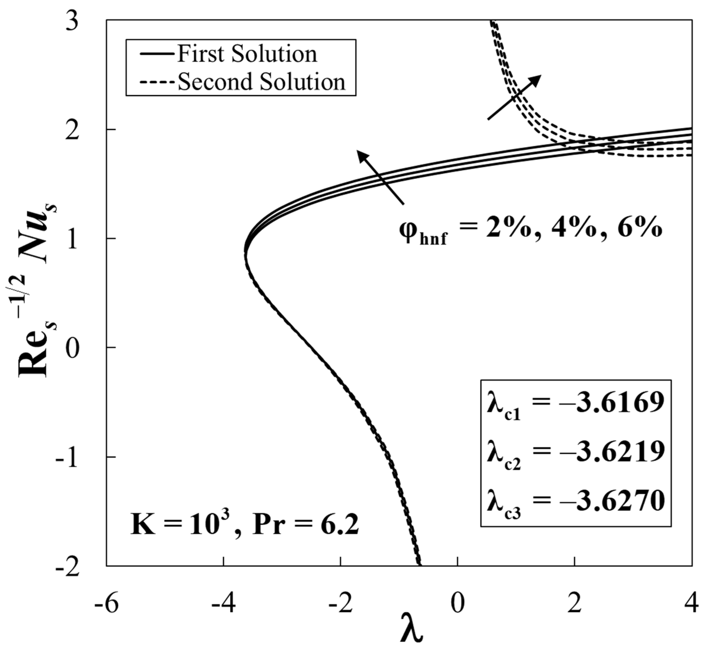
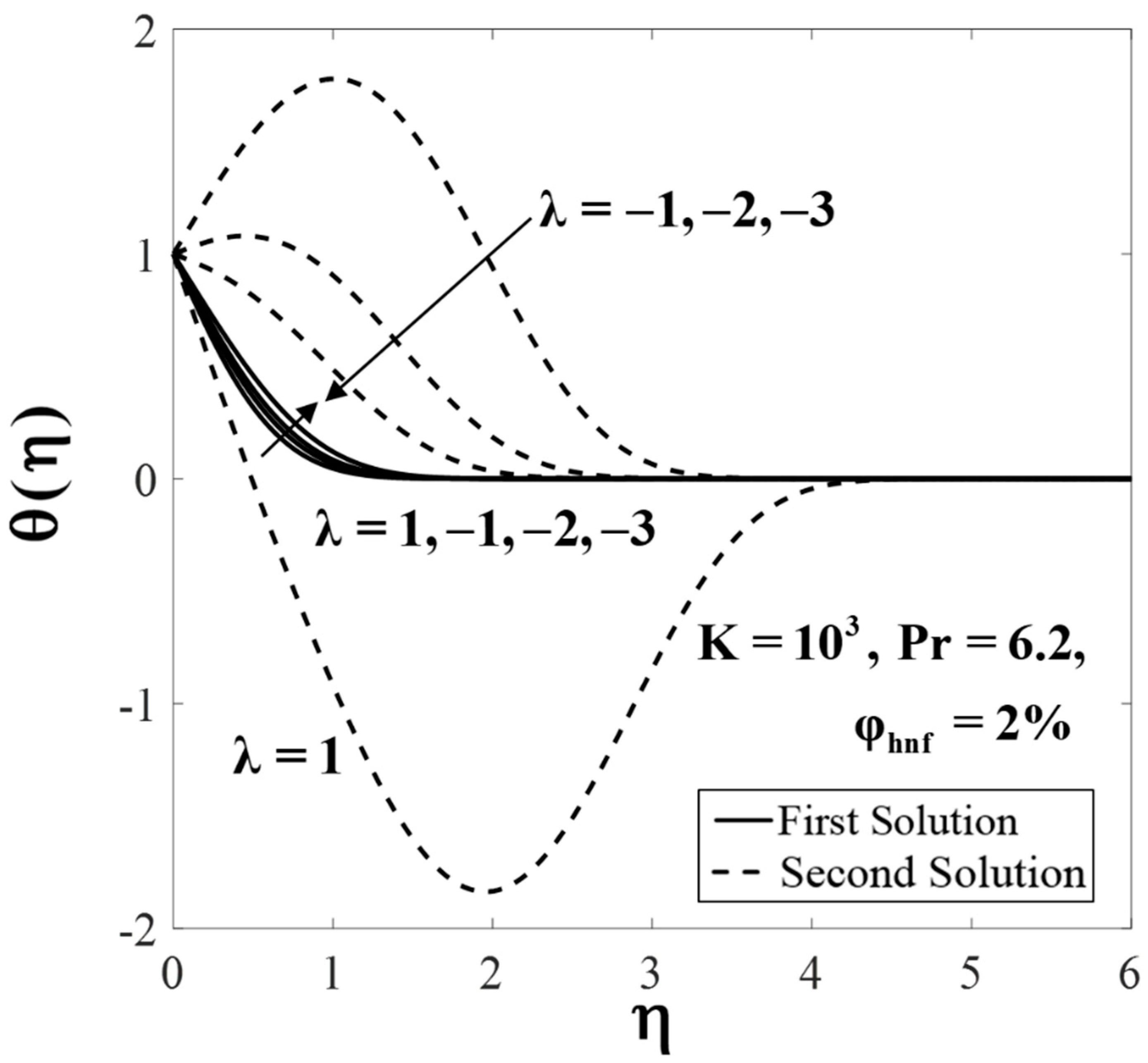
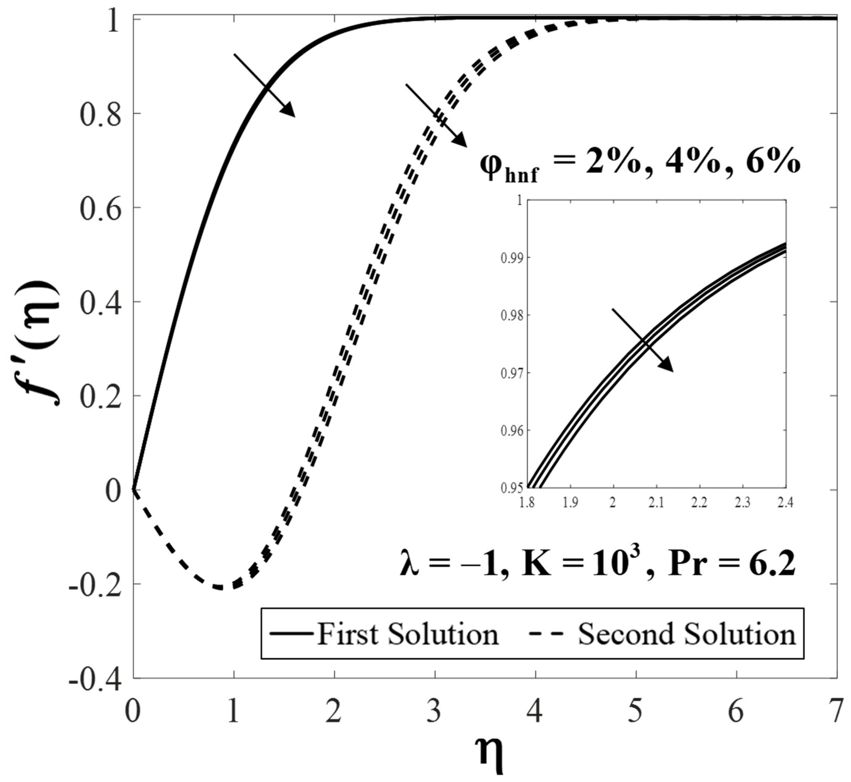
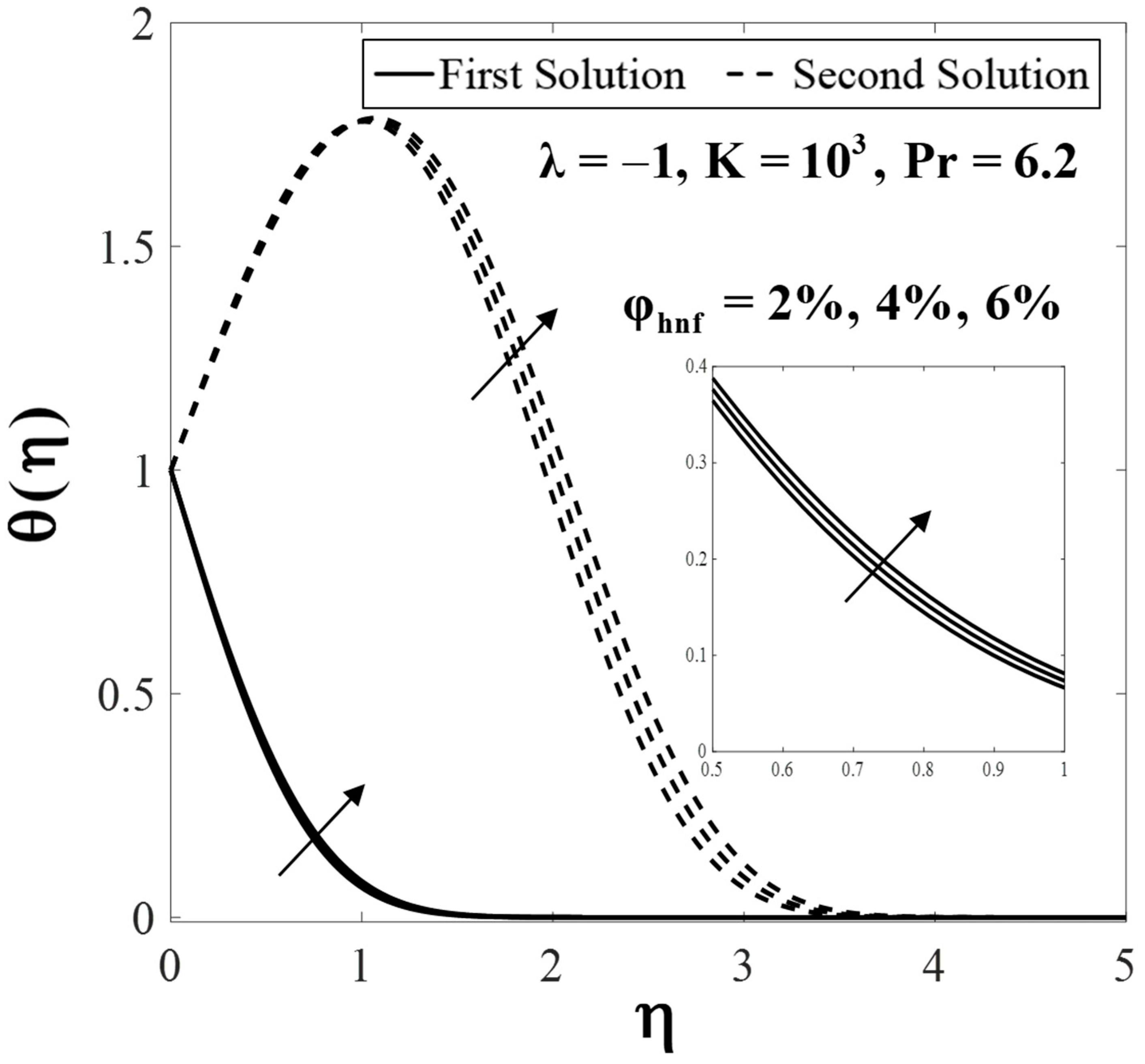
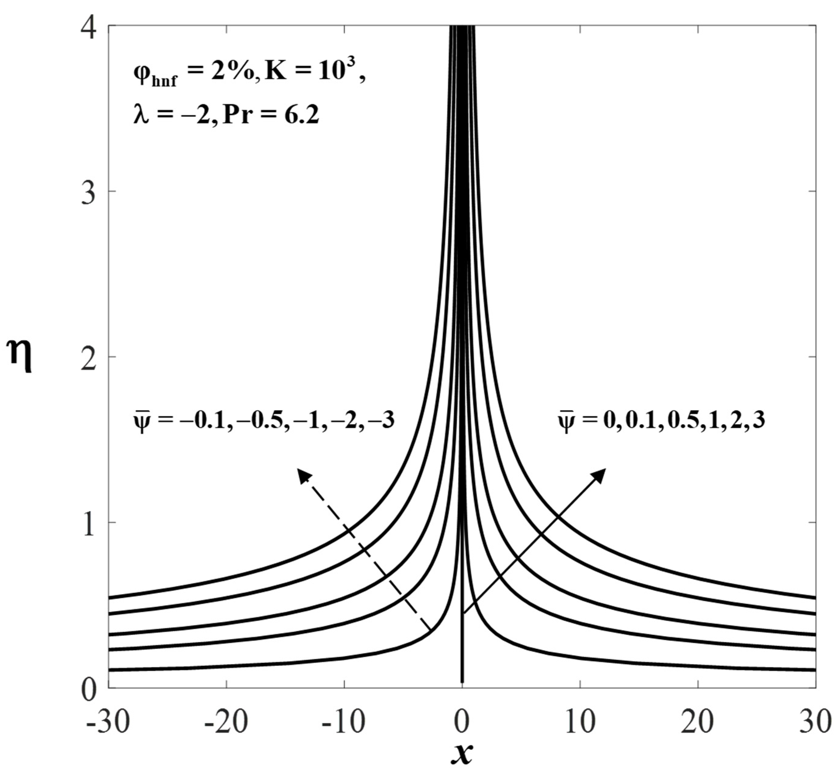
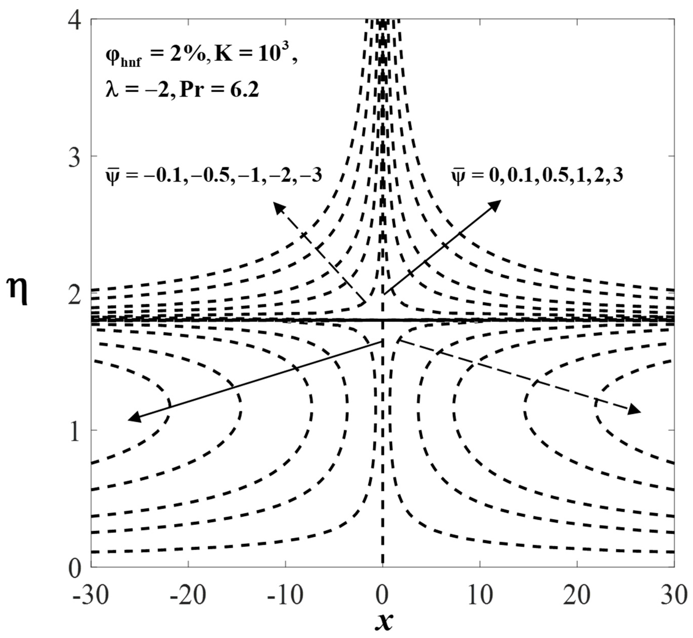
5. Results and Discussion
6. Conclusions
Author Contributions
Funding
Acknowledgments
Conflicts of Interest
References
- Hiemenz, K. Die Grenzschicht an einem in den gleichförmigen Flüssigkeitsstrom eingetauchten geraden Kreiszylinder. Dinglers Polytech. J. 1911, 326, 321–410. [Google Scholar]
- Homann, F. Der Einflub grober Zähigkeit bei der Strömung um den Zylinder und um die Kugel. Z. für Angew. Math. und Mech. 1936, 16, 153–164. [Google Scholar] [CrossRef]
- Chiam, T.C. Stagnation-point flow towards a stretching plate. J. Phys. Soc. Jpn. 1994, 63, 2443–2444. [Google Scholar] [CrossRef]
- Merkin, J.H. Mixed convection boundary layer flow on a vertical surface in a saturated porous medium. J. Eng. Math. 1980, 14, 301–313. [Google Scholar] [CrossRef]
- Ishak, A.; Nazar, R.; Arifin, N.M.; Pop, I. Dual solutions in mixed convection flow near a stagnation point on a vertical porous plate. Int. J. Therm. Sci. 2008, 47, 417–422. [Google Scholar] [CrossRef]
- Khashi’ie, N.S.; Arifin, N.M.; Rashidi, M.M.; Hafidzuddin, E.H.; Wahi, N. Magnetohydrodynamics (MHD) stagnation point flow past a shrinking/stretching surface with double stratification effect in a porous medium. J. Therm. Anal. Calorim. 2019, 8, 1–14. [Google Scholar] [CrossRef]
- Dholey, S. An unsteady separated stagnation-point flow towards a rigid flat plate. J. Fluids Eng. 2019, 141, 021202. [Google Scholar] [CrossRef]
- Fang, T.; Wang, F.; Gao, B. Unsteady magnetohydrodynamic stagnation point flow—closed-form analytical solutions. Appl. Math. Mech. 2019, 40, 449–464. [Google Scholar] [CrossRef]
- Mahapatra, T.R.; Sidui, S. Non-axisymmetric Homann stagnation-point flow of a viscoelastic fluid towards a fixed plate. Eur. J. Mech. B/Fluids 2020, 79, 38–43. [Google Scholar] [CrossRef]
- Weidman, P. Non-axisymmetric stagnation-point flow in a fluid saturated porous medium. J. Porous Media 2020, 23, 563–572. [Google Scholar] [CrossRef]
- Kumar, B.; Seth, G.S.; Nandkeolyar, R. Quadratic multiple regression model and spectral relaxation approach to analyse stagnation point nanofluid flow with second-order slip. Proc. Inst. Mech. Eng. Part E J. Process. Mech. Eng. 2020, 234, 3–14. [Google Scholar] [CrossRef]
- Choi, S.U.S.; Eastman, J.A. Enhancing thermal conductivity of fluids with nanoparticles. Proc. 1995 ASME Int. Mech. Eng. Congr. Expo. FED 231/MD 1995, 66, 99–105. [Google Scholar]
- Khanafer, K.; Vafai, K.; Lightstone, M. Buoyancy-driven heat transfer enhancement in a two-dimensional enclosure utilizing nanofluids. Int. J. Heat Mass Transf. 2003, 46, 3639–3653. [Google Scholar] [CrossRef]
- Tiwari, R.K.; Das, M.K. Heat transfer augmentation in a two-sided lid-driven differentially heated square cavity utilizing nanofluids. Int. J. Heat Mass Transf. 2007, 50, 2002–2018. [Google Scholar] [CrossRef]
- Oztop, H.F.; Abu-Nada, E. Numerical study of natural convection in partially heated rectangular enclosures filled with nanofluids. Int. J. Heat Fluid Flow 2008, 29, 1326–1336. [Google Scholar] [CrossRef]
- Hamad, M.A.A. Analytical solution of natural convection flow of a nanofluid over a linearly stretching sheet in the presence of magnetic field. Int. Commun. Heat Mass Transf. 2011, 38, 487–492. [Google Scholar] [CrossRef]
- Kameswaran, P.K.; Narayana, M.; Sibanda, P.; Murthy, P.V.S.N. Hydromagnetic nanofluid flow due to a stretching or shrinking sheet with viscous dissipation and chemical reaction effects. Int. J. Heat Mass Transf. 2012, 55, 7587–7595. [Google Scholar] [CrossRef]
- Khan, U.; Zaib, A.; Khan, I.; Nisar, K.S. Activation energy on MHD flow of titanium alloy (Ti6Al4V) nanoparticle along with a cross flow and streamwise direction with binary chemical reaction and non-linear radiation: Dual solutions. J. Mater. Res. Technol. 2020, 9, 188–199. [Google Scholar] [CrossRef]
- Waini, I.; Ishak, A.; Pop, I. Dufour and Soret effects on Al2O3-water nanofluid flow over a moving thin needle: Tiwari and Das model. Int. J. Numer. Methods Heat Fluid Flow 2021, 31, 766–782. [Google Scholar] [CrossRef]
- Majeed, A.; Zeeshan, A.; Hayat, T. Analysis of magnetic properties of nanoparticles due to applied magnetic dipole in aqueous medium with momentum slip condition. Neural Comput. Appl. 2019, 31, 189–197. [Google Scholar] [CrossRef]
- Ghosh, S.; Mukhopadhyay, S. Stability analysis for model-based study of nanofluid flow over an exponentially shrinking permeable sheet in presence of slip. Neural Comput. Appl. 2020, 32, 7201–7211. [Google Scholar] [CrossRef]
- Olayiwola, S.O.; Dejam, M. Experimental study on the viscosity behavior of silica nanofluids with different ions of electrolytes. Ind. Eng. Chem. Res. 2020, 59, 3575–3583. [Google Scholar] [CrossRef]
- Bollineni, P.K.; Dordzie, G.; Olayiwola, S.O.; Dejam, M. An experimental investigation of the viscosity behavior of solutions of nanoparticles, surfactants, and electrolytes. Phys. Fluids 2021, 33, 026601. [Google Scholar] [CrossRef]
- Sidik, N.A.C.; Adamu, I.M.; Jamil, M.M.; Kefayati, G.H.R.; Mamat, R.; Najafi, G. Recent progress on hybrid nanofluids in heat transfer applications: A comprehensive review. Int. Commun. Heat Mass Transf. 2016, 78, 68–79. [Google Scholar] [CrossRef]
- Turcu, R.; Darabont, A.; Nan, A.; Aldea, N.; Macovei, D.; Bica, D.; Vekas, L.; Pana, O.; Soran, M.L.; Koos, A.A.; et al. New polypyrrole-multiwall carbon nanotubes hybrid materials. J. Optoelectron. Adv. Mater. 2006, 8, 643–647. [Google Scholar]
- Jana, S.; Salehi-Khojin, A.; Zhong, W.H. Enhancement of fluid thermal conductivity by the addition of single and hybrid nano-additives. Thermochim. Acta 2007, 462, 45–55. [Google Scholar] [CrossRef]
- Suresh, S.; Venkitaraj, K.P.; Selvakumar, P.; Chandrasekar, M. Synthesis of Al2O3-Cu/water hybrid nanofluids using two step method and its thermo physical properties. Colloids Surf. A Physicochem. Eng. Asp. 2011, 388, 41–48. [Google Scholar] [CrossRef]
- Singh, S.K.; Sarkar, J. Energy, exergy and economic assessments of shell and tube condenser using hybrid nanofluid as coolant. Int. Commun. Heat Mass Transf. 2018, 98, 41–48. [Google Scholar] [CrossRef]
- Farhana, K.; Kadirgama, K.; Rahman, M.M.; Noor, M.M.; Ramasamy, D.; Samykano, M.; Najafi, G.; Sidik, N.A.C.; Tarlochan, F. Significance of alumina in nanofluid technology: An overview. J. Therm. Anal. Calorim. 2019, 138, 1107–1126. [Google Scholar] [CrossRef]
- Takabi, B.; Salehi, S. Augmentation of the heat transfer performance of a sinusoidal corrugated enclosure by employing hybrid nanofluid. Adv. Mech. Eng. 2014, 6, 147059. [Google Scholar] [CrossRef]
- Kumar, V.; Sarkar, J. Particle ratio optimization of Al2O3-MWCNT hybrid nanofluid in minichannel heat sink for best hydrothermal performance. Appl. Therm. Eng. 2020, 165, 114546. [Google Scholar] [CrossRef]
- Salehi, S.; Nori, A.; Hosseinzadeh, K.; Ganji, D.D. Hydrothermal analysis of MHD squeezing mixture fluid suspended by hybrid nanoparticles between two parallel plates. Case Stud. Therm. Eng. 2020, 21, 100650. [Google Scholar] [CrossRef]
- Muhammad, K.; Hayat, T.; Alsaedi, A.; Ahmad, B. Melting heat transfer in squeezing flow of basefluid (water), nanofluid (CNTs + water) and hybrid nanofluid (CNTs + CuO + water). J. Therm. Anal. Calorim. 2021, 143, 1157–1174. [Google Scholar] [CrossRef]
- Waini, I.; Ishak, A.; Pop, I. Hybrid nanofluid flow over a permeable non-isothermal shrinking surface. Mathematics 2021, 9, 538. [Google Scholar] [CrossRef]
- Khan, U.; Waini, I.; Ishak, A.; Pop, I. Unsteady hybrid nanofluid flow over a radially permeable shrinking/stretching surface. J. Mol. Liq. 2021, 331, 115752. [Google Scholar] [CrossRef]
- Sarkar, J.; Ghosh, P.; Adil, A. A review on hybrid nanofluids: Recent research, development and applications. Renew. Sustain. Energy Rev. 2015, 43, 164–177. [Google Scholar] [CrossRef]
- Babu, J.A.R.; Kumar, K.K.; Rao, S.S. State-of-art review on hybrid nanofluids. Renew. Sustain. Energy Rev. 2017, 77, 551–565. [Google Scholar] [CrossRef]
- Sajid, M.U.; Ali, H.M. Thermal conductivity of hybrid nanofluids: A critical review. Int. J. Heat Mass Transf. 2018, 126, 211–234. [Google Scholar] [CrossRef]
- Huminic, G.; Huminic, A. Entropy generation of nanofluid and hybrid nanofluid flow in thermal systems: A review. J. Mol. Liq. 2020, 302, 112533. [Google Scholar] [CrossRef]
- Yang, L.; Ji, W.; Mao, M.; Huang, J. An updated review on the properties, fabrication and application of hybrid-nanofluids along with their environmental effects. J. Clean. Prod. 2020, 257, 120408. [Google Scholar] [CrossRef]
- Sajid, M.; Ali, N.; Javed, T.; Abbas, Z. Stretching a curved surface in a viscous fluid. Chin. Phys. Lett. 2010, 27, 024703. [Google Scholar] [CrossRef]
- Sajid, M.; Ali, N.; Abbas, Z.; Javed, T. Flow of a micropolar fluid over a curved stretching surface. J. Eng. Phys. Thermophys. 2011, 84, 864–871. [Google Scholar] [CrossRef]
- Abbas, Z.; Naveed, M.; Sajid, M. Heat transfer analysis for stretching flow over a curved surface with magnetic field. J. Eng. Thermophys. 2013, 22, 337–345. [Google Scholar] [CrossRef]
- Abbas, Z.; Naveed, M.; Sajid, M. Hydromagnetic slip flow of nanofluid over a curved stretching surface with heat generation and thermal radiation. J. Mol. Liq. 2016, 215, 756–762. [Google Scholar] [CrossRef]
- Hayat, T.; Kiran, A.; Imtiaz, M.; Alsaedi, A. Hydromagnetic mixed convection flow of copper and silver water nanofluids due to a curved stretching sheet. Results Phys. 2016, 6, 904–910. [Google Scholar] [CrossRef][Green Version]
- Imtiaz, M.; Hayat, T.; Alsaedi, A. Convective flow of ferrofluid due to a curved stretching surface with homogeneous-heterogeneous reactions. Powder Technol. 2017, 310, 154–162. [Google Scholar] [CrossRef]
- Saba, F.; Ahmed, N.; Hussain, S.; Khan, U.; Mohyud-Din, S.; Darus, M. Thermal analysis of nanofluid flow over a curved stretching surface suspended by carbon nanotubes with internal heat generation. Appl. Sci. 2018, 8, 395. [Google Scholar] [CrossRef]
- Sanni, K.M.; Asghar, S.; Jalil, M.; Okechi, N.F. Flow of viscous fluid along a nonlinearly stretching curved surface. Results Phys. 2017, 7, 1–4. [Google Scholar] [CrossRef]
- Hayat, T.; Saif, R.S.; Ellahi, R.; Muhammad, T.; Ahmad, B. Numerical study of boundary-layer flow due to a nonlinear curved stretching sheet with convective heat and mass conditions. Results Phys. 2017, 7, 2601–2606. [Google Scholar] [CrossRef]
- Okechi, N.F.; Jalil, M.; Asghar, S. Flow of viscous fluid along an exponentially stretching curved surface. Results Phys. 2017, 7, 2851–2854. [Google Scholar] [CrossRef]
- Saleh, S.H.M.; Arifin, N.M.; Nazar, R.; Pop, I. Unsteady micropolar fluid over a permeable curved stretching shrinking surface. Math. Probl. Eng. 2017, 2017, 3085249. [Google Scholar] [CrossRef]
- Naveed, M.; Abbas, Z.; Sajid, M.; Hasnain, J. Dual solutions in hydromagnetic viscous fluid flow past a shrinking curved surface. Arab. J. Sci. Eng. 2018, 43, 1189–1194. [Google Scholar] [CrossRef]
- Khan, M.R.; Pan, K.; Khan, A.U.; Nadeem, S. Dual solutions for mixed convection flow of SiO2−Al2O3/water hybrid nanofluid near the stagnation point over a curved surface. Phys. A Stat. Mech. its Appl. 2020, 547, 123959. [Google Scholar] [CrossRef]
- Lok, Y.Y.; Amin, N.; Campean, D.; Pop, I. Steady mixed convection flow of a micropolar fluid near the stagnation point on a vertical surface. Int. J. Numer. Methods Heat Fluid Flow 2005, 15, 654–670. [Google Scholar] [CrossRef]
- Merkin, J.H. On dual solutions occurring in mixed convection in a porous medium. J. Eng. Math. 1986, 20, 171–179. [Google Scholar] [CrossRef]
- Weidman, P.D.; Kubitschek, D.G.; Davis, A.M.J. The effect of transpiration on self-similar boundary layer flow over moving surfaces. Int. J. Eng. Sci. 2006, 44, 730–737. [Google Scholar] [CrossRef]
- Shampine, L.F.; Gladwell, I.; Thompson, S. Solving ODEs with MATLAB; Cambridge University Press: Cambridge, UK, 2003. [Google Scholar]


| Properties | Base Fluid | Nanoparticles | |
|---|---|---|---|
| Water | Al2O3 | SiO2 | |
| 997.1 | 3970 | 2200 | |
| 4179 | 765 | 745 | |
| 0.613 | 40 | 1.4 | |
| 21 | 0.85 | 42.7 | |
| Prandtl number, | 6.2 | ||
| Properties | Correlations |
|---|---|
| Dynamic viscosity | |
| Density | |
| Heat capacity | |
| Thermal conductivity | |
| Thermal expansion |
| Lok Et Al. [54] | Present Results | |||
|---|---|---|---|---|
| −1.0 | 0.691693 | 0.633269 | 0.691661 | 0.633247 |
| (−0.285049) | (−0.222165) | |||
| −1.5 | 0.371788 | 0.578230 | 0.371754 | 0.578206 |
| (−0.527666) | (−0.004360) | (−0.527651) | (−0.004347) | |
| −2.0 | −0.039513 | 0.486576 | −0.039572 | 0.486540 |
| (−0.578523) | (0.198572) | (−0.578476) | (0.198599) | |
| First Solution | Second Solution | First Solution | Second Solution | ||
|---|---|---|---|---|---|
| 2% | 1 | 1.609474 | 0.652232 | 1.708511 | 2.232347 |
| 4% | 1.684045 | 0.691249 | 1.759909 | 2.317150 | |
| 6% | 1.761695 | 0.731805 | 1.811141 | 2.401796 | |
| 2% | −1 | 0.969496 | −0.380839 | 1.530307 | −1.239090 |
| −2 | 0.594987 | −0.642901 | 1.403953 | −0.295385 | |
| −3 | 0.131804 | −0.707488 | 1.208754 | 0.282748 | |
Publisher’s Note: MDPI stays neutral with regard to jurisdictional claims in published maps and institutional affiliations. |
© 2021 by the authors. Licensee MDPI, Basel, Switzerland. This article is an open access article distributed under the terms and conditions of the Creative Commons Attribution (CC BY) license (https://creativecommons.org/licenses/by/4.0/).
Share and Cite
Waini, I.; Ishak, A.; Pop, I. Flow towards a Stagnation Region of a Curved Surface in a Hybrid Nanofluid with Buoyancy Effects. Mathematics 2021, 9, 2330. https://doi.org/10.3390/math9182330
Waini I, Ishak A, Pop I. Flow towards a Stagnation Region of a Curved Surface in a Hybrid Nanofluid with Buoyancy Effects. Mathematics. 2021; 9(18):2330. https://doi.org/10.3390/math9182330
Chicago/Turabian StyleWaini, Iskandar, Anuar Ishak, and Ioan Pop. 2021. "Flow towards a Stagnation Region of a Curved Surface in a Hybrid Nanofluid with Buoyancy Effects" Mathematics 9, no. 18: 2330. https://doi.org/10.3390/math9182330
APA StyleWaini, I., Ishak, A., & Pop, I. (2021). Flow towards a Stagnation Region of a Curved Surface in a Hybrid Nanofluid with Buoyancy Effects. Mathematics, 9(18), 2330. https://doi.org/10.3390/math9182330