Dynamic Optimal Mean-Variance Investment with Mispricing in the Family of 4/2 Stochastic Volatility Models

Abstract

This paper considers an optimal investment problem with mispricing in the family of 4/2 stochastic volatility models under mean–variance criterion. The financial market consists of a risk-free asset, a market index and a pair of mispriced stocks. By applying the linear–quadratic stochastic control theory and solving the corresponding Hamilton–Jacobi–Bellman equation, explicit expressions for the statically optimal (pre-commitment) strategy and the corresponding optimal value function are derived. Moreover, a necessary verification theorem was provided based on an assumption of the model parameters with the investment horizon. Due to the time-inconsistency under mean–variance criterion, we give a dynamic formulation of the problem and obtain the closed-form expression of the dynamically optimal (time-consistent) strategy. This strategy is shown to keep the wealth process strictly below the target (expected terminal wealth) before the terminal time. Results on the special case without mispricing are included. Finally, some numerical examples are given to illustrate the effects of model parameters on the efficient frontier and the difference between static and dynamic optimality.

1. Introduction

The development of continuous-time stochastic volatility models is deemed crucial in the field of modern finance. The attraction of stochastic volatility models mainly resides in their capacity to explain many stylized facts observed in the financial market such as fat tails, the leverage effect and the volatility smile/skew on implied volatility surfaces. See, for example, Hull and White [1], Stein and Stein [2], Heston [3] and Lewis [4]. In 2017, Grasselli [5] proposed a new model called the 4/2 stochastic volatility model which embraces the celebrated Heston model and the 3/2 model (Lewis [4]) as special cases. The superposition of these two parsimonious models makes it possible for the new 4/2 model to better predict the evolution of the implied volatility surface. This leads to emerging interests in applications of Grasselli’s work to derivative pricing problems, such as Cui et al. [6], Cui et al. [7] and Zhu and Wang [8]. In view of the success of the 4/2 model in terms of option pricing, Cheng and Escobar-Anel [9] recently investigated a utility maximization problem under the 4/2 model. It seems, however, that little attention has been paid to portfolio optimization problems with the 4/2 model under Markowitz [10]’s mean–variance criterion.

The single-period portfolio selection problem under mean–variance criterion can be traced back to the seminar work of Markowitz [10]. Li and Ng [11] and Zhou and Li [12] generalized Markowitz’s work to multi-period and continuous settings, respectively. In particular, Zhou and Li [12] applied the standard results on the linear–quadratic stochastic control theory combined with an embedding technique to solve the problem in a financial market where all the market coefficients are deterministic. Many researchers then realized the potential of diversification. For example, Shen et al. [13] solved the problem under the constant elasticity of the variance model by imposing an exponential integrability condition on the market price of risk. Shen and Zeng [14] went a step forward by considering the optimal investment–reinsurance problem for a mean–variance insurer in an incomplete market where the market price of risk depends on an affine-form and square-root process, and they derived the modified locally square-integrable optimal strategy. Sun et al. [15] further extended Shen and Zeng [14]’s results to the case with multiple risky assets and random liabilities. For other previous works, one can refer to Chiu and Wong [16], Yu [17], Lv et al. [18], Tian et al. [19], Sun and Guo [20] and the references therein.

In the aforementioned literature, however, the optimal strategies depend on the initial position of state variables, which is due to the non-separability of the variance operator under mean–variance criterion in the sense of Bellman’s optimality principle. In other words, once the investor arrives at any new position at a future time, the optimal strategy determined at the new position is inconsistent with the initial one unless the investor commits to the initial strategy over the whole investment period. This optimal strategy is therefore time-inconsistent, and is referred to as the pre-commitment strategy in the literature. The notion of time-inconsistency under mean–variance paradigm stemmed from the work of Strotz [21]. In recent years, the time-inconsistency of the mean–variance portfolio selection problem has received considerable attention. For example, Basak and Chabakauri [22] determined a time-consistent strategy by using a backward recursion approach starting from the terminal time. Alternatively, Björk et al. [23] proposed the game theoretical approach and studied the subgame-perfect Nash equilibrium for the mean–variance problem. The equilibrium value function and the equilibrium strategy can be explicitly derived under Markovian settings by essentially solving an extended Hamilton–Jacobi–Bellman (HJB) equation. Rather than searching for the time-consistent equilibrium strategy, Pedersen and Peskir [24] pioneered the dynamically optimal approach to deal with the time-inconsistency of the statically optimal (pre-commitment) strategy. Along with this approach, previous works include Pedersen and Peskir [25], Zhang [26] and the references therein.

According to the law of one price, identical assets must have an identical price. There is, however, ample evidence of violations in the law of one price and of the prevalence of a mispricing phenomenon in the financial market. See, for example, Lamont and Thaler [27], Liu and Longstaff [28] and Liu and Timmermann [29]. This leads to growing interests in portfolio optimization problems with mispricing in recent years. Yi et al. [30] studied a utility maximization problem with model ambiguity and mispricing in a financial market consisting of a risk-free asset, a market index, and a pair of mispricing stocks with the constant return rate and volatility. Ma et al. [31] considered a problem for a defined contribution plan with mispricing under the Heston model. Considering the methodology developed by Björk et al. [23] to deal with the time inconsistency under mean–variance paradigm, Wang et al. [32] investigated a mean–variance investment–reinsurance problem with mispricing in the context of constant volatility. Other preceding research outputs on the portfolio optimization problems with mispricing include Gu, Viens and Yi [33], Gu, Viens and Yao [34], Wang et al. [35], to name but only a few.

Motivated by the above aspects, within the framework introduced by Pedersen and Peskir [24] to overcome the time inconsistency under mean–variance criterion, in this paper we study a mean–variance portfolio selection problem that takes into consideration the family of 4/2 stochastic volatility models and mispricing simultaneously. The financial market consists of a risk-free asset, a market index and a pair of mispriced stocks. To solve this problem, we first apply the Lagrange multiplier method to relate the original problem to an unconstrained optimization problem. To solve the latter by using the dynamic programming approach, we establish the corresponding HJB equation. By solving the HJB equation explicitly, closed-form expressions of the statically optimal strategy and the corresponding optimal value function are derived. Based on an assumption on the model parameters combined with the investment horizon, we prove the necessary verification theorem from scratch and verify the admissibility of the optimal strategy. By solving the statically optimal strategy each time, the dynamically optimal strategy is explicitly derived. This time-consistent strategy keeps the wealth process strictly below the target (expected terminal wealth) before the terminal time. Moreover, we provide the results without mispricing and consider the special cases under the Heston and the 3/2 models. Finally, we present some numerical examples to illustrate the effects of some model parameters on the efficient frontier and the difference between static and dynamic optimality. In summary, compared with some related current research studies, the main contributions of this paper are as follows:

• The market model incorporates the 4/2 model and mispricing simultaneously;
• By making an assumption on the model parameters, a verification theorem is provided to guarantee that the candidate solution to the HJB equation is the optimal value function, and the admissibility of the optimal strategy is verified;
• We derive both the statically optimal (pre-commitment) and the dynamically optimal (time-consistent) strategies explicitly for the mean–variance problem.

The remainder of this paper is structured as follows. In Section 2, we formulate the market model and the mean–variance portfolio problem. Section 3 is devoted to solving the HJB equation and deriving the closed-form expression of the optimal investment strategy of the unconstrained problem. In Section 4, we present the statically optimal strategy and the dynamically optimal strategy for the mean–variance problem, and provide the results on some special cases. In Section 5, some numerical examples are given to illustrate our theoretical results. Section 6 concludes the paper.

2. Formulation of the Problem

Let $T>0$ be a fixed terminal time of decision making and $(\mathsf{\Omega },\mathcal{F},\mathrm{P})$ be a complete probability space carrying five one-dimensional, mutually independent standard Brownian motions $W^1,W^2,Z,Z^1,Z^2$. The probability space is further equipped with a right-continuous, $\mathrm{P}$-complete filtration ${\left({\mathcal{F}}_t\right)}_{t\in [0,T]}$ generated by the Brownian motions.

We consider a financial market setting where a risk-free asset, a market index, and a pair of stocks with mispricing can be continuously traded. The risk-free asset price $B={\left(B_t\right)}_{t\in [t_0,T]}$ evolves over time as:

$$d{B}_t=r{B}_{t}dt,$$

with the initial value $B_{t_0}=b_0\in {\mathbb{R}}^{+}$ at time $t_0\in [0,T)$, where the positive constant $r>0$ is the risk-free interest rate. Let the price dynamic of the market index $S_m={\left(S_{m,t}\right)}_{t\in [t_0,T]}$ be governed by the 4/2 stochastic volatility model (Grasselli [5]):

$$\begin{array}{c}\hfill \left\{\begin{array}{cc}\hfill d{S}_{m,t}& =\left(r+\lambda (c_1{V}_t+c_2)\right)S_{m,t}dt+\left(c_1\sqrt{V_t}+\frac{c_2}{\sqrt{V_t}}\right)S_{m,t}d{W}_t^1,\hfill \\ \hfill d{V}_t& =\kappa ({\theta }_v-V_t)dt+{\sigma }_v\sqrt{V_t}\left(\rho d{W}_t^1+\sqrt{1-{\rho }^2}d{W}_t^2\right),\hfill \end{array}\right.\end{array}$$

(1)

with $S_{m,t_0}=s_{m,0}\in {\mathbb{R}}^{+}$ and $V_{t_0}=v_0\in {\mathbb{R}}^{+}$ at time $t_0\in [0,T)$, where the constant $\lambda >0$ stands for a controller of the excess return, and the variance process $V_t$ follows a Cox–Ingersoll–Ross (CIR) process with mean-reversion speed $\kappa >0$, long-term mean ${\theta }_v>0$ and volatility of volatility ${\sigma }_v>0$. The Feller condition $2\kappa {\theta }_v>{\sigma }_v^2$ is required such that $V_t$ is strictly positive. We assume that two parameters $c_1$ and $c_2$ are non-negative constants and $\rho \in [-1,1]$.

Remark 1.

It should be noted that the two non-negative constants $c_1\ge 0$ and $c_2\ge 0$ are critical in the 4/2 model (1), which makes the 4/2 model a superposition of the Heston model (Heston [3]) and the 3/2 model (Lewis [4]). Specifically, the case $(c_1,c_2)=(1,0)$ is known as the Heston model, while the case $(c_1,c_2)=(0,1)$ corresponds to the 3/2 model.

The two mispriced processes are modeled as a pair of stocks $S_1={\left(S_{1,t}\right)}_{t\in [t_0,T]}$ and $S_2={\left(S_{2,t}\right)}_{t\in [t_0,T]}$ which are coupled via the pricing error:

$$M_t=ln\frac{S_{1,t}}{S_{2,t}},$$

where $S_{1,t}$ and $S_{2,t}$ evolve according to the following system of stochastic differential equations (SDEs):

$$\begin{array}{c}\hfill \left\{\begin{array}{cc}\hfill d{S}_{1,t}=& (r+\beta \lambda (c_1{V}_t+c_2))S_{1,t}dt+\beta \left(c_1\sqrt{V_t}+\frac{c_2}{\sqrt{V_t}}\right)S_{1,t}d{W}_t^1\hfill \\ & +\sigma S_{1,t}d{Z}_t+b{S}_{1,t}d{Z}_t^1-l_1{M}_t{S}_{1,t}dt,\hfill \\ \hfill d{S}_{2,t}=& (r+\beta \lambda (c_1{V}_t+c_2))S_{2,t}dt+\beta \left(c_1\sqrt{V_t}+\frac{c_2}{\sqrt{V_t}}\right)S_{2,t}d{W}_t^1\hfill \\ & +\sigma S_{2,t}d{Z}_t+b{S}_{2,t}d{Z}_t^2+l_2{M}_t{S}_{2,t}dt,\hfill \end{array}\right.\end{array}$$

(2)

with initial values $S_{1,t_0}=s_{1,0}$ and $S_{2,t_0}=s_{2,0}$ at time $t_0\in [0,T)$, where $l_1,l_2,\beta ,\sigma$ and b are constant parameters. The term $\beta \left(c_1\sqrt{V_t}+\frac{c_2}{\sqrt{V_t}}\right)d{W}_t^1$ characterizes the systematic risk of the market, while $\sigma d{Z}_t+bd{Z}_t^i$ stands for the idiosyncratic risk of stock i, $i=1,2$. In particular, $\sigma d{Z}_t$ describes the common risk whereas $bd{Z}_t^i$ represents the individual risk generated by the stock i, $i=1,2$, respectively. The term $l_i{M}_t$ reveals the effect of mispricing on ith stock’s price via the pricing error $M_t$ defined above. Moreover, it can be shown that the pricing error $M_t$ follows an Ornstein–Uhlenbeck (OU) process as a result of Itô’s formula:

$$d{M}_t=-(l_1+l_2)M_{t}dt+bd{Z}_t^1-bd{Z}_t^2,$$

(3)

with $M_{t_0}=m_0=ln(s_{1,0}/s_{2,0})\in \mathbb{R}$, where two constant parameters $l_1$ and $l_2$ can be explained as liquidity terms which control the mean-reversion rate of the pricing error. To be specific, the lower liquidity decreases the velocity of reversion of the pricing error towards the long-term mean of zero. Following some previous studies, such as Liu and Timmermann [29], Ma et al. [31] and Wang et al. [32], we hereby assume that $l_1+l_2>0$, which ensures the stability of the financial market.

Let ${\pi }_m(t,V_t,M_t,X_t^{\pi })$, ${\pi }_1(t,V_t,M_t,X_t^{\pi }),{\pi }_2(t,V_t,M_t,X_t^{\pi })$ be three Markov controls denoting the proportions of wealth invested in the market index $S_m$, and the pair of stocks $S_1$ and $S_2$ at time t, respectively. We write $\pi :=({\pi }_m,{\pi }_1,{\pi }_2)$ and such deterministic functions ${\pi }_m,{\pi }_1,{\pi }_2$ are referred to as feedback control laws in the literature. Suppose that the market is frictionless and no restrictions on leverage and short-selling are enforced, the investor decides to construct a self-financing portfolio of $B,S_m,S_1$ and $S_2$ over the investment period $[t_0,T]$. So the controlled wealth process $X^{\pi }={\left(X_t^{\pi }\right)}_{t\in [t_0,T]}$ is described by the following system of SDEs:

$$\begin{array}{c}\hfill \left\{\begin{array}{cc}\hfill d{X}_t^{\pi }=& X_t^{\pi }\left[r+u_m(t,V_t,M_t,X_t^{\pi })\lambda (c_1{V}_t+c_2)-({\pi }_1(t,V_t,M_t,X_t^{\pi })l_1\right.\hfill \\ & \left.-{\pi }_2(t,V_t,M_t,X_t^{\pi })l_2)M_t\right]dt+X_t^{\pi }\left(c_1\sqrt{V_t}+\frac{c_2}{\sqrt{V_t}}\right)u_m(t,V_t,M_t,X_t^{\pi })d{W}_t^1\hfill \\ \hfill & +X_t^{\pi }\sigma ({\pi }_1(t,V_t,M_t,X_t^{\pi })+{\pi }_2(t,V_t,M_t,X_t^{\pi }))d{Z}_t\hfill \\ \hfill & +X_t^{\pi }b\left({\pi }_1(t,V_t,M_t,X_t^{\pi })d{Z}_t^1+{\pi }_2(t,V_t,M_t,X_t^{\pi })d{Z}_t^2\right),\hfill \\ \hfill d{V}_t=& \kappa ({\theta }_v-V_t)dt+{\sigma }_v\sqrt{V_t}\left(\rho d{W}_t^1+\sqrt{1-{\rho }^2}d{W}_t^2\right),\hfill \\ \hfill d{M}_t=& -(l_1+l_2)M_{t}dt+bd{Z}_t^1-bd{Z}_t^2,\hfill \end{array}\right.\end{array}$$

(4)

with $X_{t_0}^{\pi }=x_0$, where we write $u_m:={\pi }_m+\beta ({\pi }_1+{\pi }_2)$ to simplify our notation. Let ${\mathrm{P}}_{t_0,v_0,m_0,x_0}$ denote the probability measure with the initial value $(V_{t_0},M_{t_0},X_{t_0}^{\pi })=(v_0,m_0,x_0)$ at time $t_0\in [0,T)$. Accordingly, ${\mathrm{E}}_{t_0,v_0,m_0,x_0}[·]$ and ${\mathrm{Var}}_{t_0,v_0,m_0,x_0}(·)$ denote the associated expectation and variance under the probability measure ${\mathrm{P}}_{t_0,v_0,m_0,x_0}$, respectively.

Definition 1

(Admissible strategy). Given any fixed $t_0\in [0,T)$, a strategy π is said to be admissible if for any $(v_0,m_0,x_0)\in {\mathbb{R}}^{+}\times \mathbb{R}\times \mathbb{R}$, it holds that:

1. 

${\mathrm{E}}_{t_0,v_0,m_0,x_0}\left[{\int }_{t_0}^T{\left(X_t^{\pi }\right)}^2{\left(c_1\sqrt{V_t}+\frac{c_2}{\sqrt{V_t}}\right)}^2{u}_m^2(t,V_t,M_t,X_t^{\pi })dt\right]<\infty$,

2. 

${\mathrm{E}}_{t_0,v_0,m_0,x_0}\left[{\int }_{t_0}^T{\left(X_t^{\pi }\right)}^2\left({\pi }_1^2(t,V_t,M_t,X_t^{\pi })+{\pi }_2^2(t,V_t,M_t,X_t^{\pi })\right)dt\right]<\infty$,

3. 

${\mathrm{E}}_{t_0,v_0,m_0,x_0}\left[{sup}_{t\in [t_0,T]}{\left|X_t^{\pi }\right|}^2\right]<\infty$.

The set of all admissible strategies is denoted by $\mathcal{A}$.

The investor wishes to determine an admissible strategy $\pi \in \mathcal{A}$ solving the following mean–variance portfolio problem.

Definition 2.

The mean–variance portfolio problem is a stochastic optimization problem denoted by

$$\begin{array}{c}\hfill \left\{\begin{array}{cc}\hfill \underset{\pi \in \mathcal{A}}{min}& {\mathrm{Var}}_{t_0,v_0,m_0,x_0}\left(X_T^{\pi }\right)\hfill \\ \hfill \mathrm{subject}\mathrm{to}& {\mathrm{E}}_{t_0,v_0,m_0,x_0}\left[X_T^{\pi }\right]=\xi ,\hfill \end{array}\right.\end{array}$$

(5)

where ξ is a fixed and given constant serving as a target. We denote the corresponding optimal value function by $V_{MV}(t_0,v_0,m_0,x_0)$.

Remark 2.

Here, we impose $\xi >x_0{e}^{r(T-t_0)}$, which precludes the trivial case when the investor simply takes the risk-free strategy $\pi \equiv 0$ over the investment period $[t_0,T]$. This condition is consistent with some previous studies, such as Shen et al. [13], Sun and Guo [20] and Sun et al. [15].

As discussed in the Introduction, the mean–variance problem (5) is time-inconsistent due to the presence of the variance operator in the mean–variance objective. We take the dynamically optimal approach as championed by Pedersen and Peskir [24] to address the problem of time-inconsistency. For readers’ convenience, we adapted the definition of the dynamic optimality (Definition 2 in Pedersen and Peskir [24]) into the current context.

Definition 3

(Dynamic optimality). A control ${\pi }^{d*}$ is said to be dynamically optimal in mean–variance portfolio problem (5) for $(t_0,v_0,m_0,x_0)$ given and fixed, if for every given and fixed $(t,v,m,x)\in [t_0,T)\times {\mathbb{R}}^{+}\times \mathbb{R}\times \mathbb{R}$ and every strategy $u\in \mathcal{A}$ such that $u(t,v,m,x)\ne {\pi }^{d*}(t,v,m,x)$ with ${\mathrm{E}}_{t,v,m,x}\left[X_T^u\right]=\xi$, there exists a control w satisfying $w(t,v,m,x)={\pi }^{d*}(t,v,m$, $x)$ with ${\mathrm{E}}_{t,v,m,x}\left[X_T^w\right]=\xi$ such that

$${\mathrm{Var}}_{t,v,m,x}\left(X_T^w\right)<{\mathrm{Var}}_{t,v,m,x}\left(X_T^{\pi }\right).$$

Upon considering the nature of the dynamically optimal approach, as discussed in the Introduction, we shall first pay attention to the static optimality (pre-commitment) for the mean–variance problem (5).

Due to the convexity of the objective function in the problem (5), we can deal with the linear constraint ${\mathrm{E}}_{t_0,v_0,m_0,x_0}\left[X_T^{\pi }\right]=\xi$ by introducing a Lagrange multiplier $\theta \in \mathbb{R}$. The associated (dual) Lagrangian is formulated as follows:

$$\begin{array}{cc}\hfill L(x_0,v_0,m_0;\pi ,\theta )=& {\mathrm{E}}_{t_0,v_0,m_0,x_0}\left[{(X_T^{\pi }-\xi )}^2\right]+2\theta {\mathrm{E}}_{t_0,v_0,m_0,x_0}[X_T^{\pi }-\xi ]\hfill \\ \hfill =& {\mathrm{E}}_{t_0,v_0,m_0,x_0}\left[{(X_T^{\pi }-(\xi -\theta ))}^2\right]-{\theta }^2.\hfill \end{array}$$

(6)

According to the Lagrangian duality theorem (Luenberger [36]), the mean–variance problem (5) is, in fact, equivalent to the following min–max stochastic optimization problem:

$$\underset{\theta \in \mathbb{R}}{max}\underset{\pi \in \mathcal{A}}{min}L(x_0,v_0,m_0;\pi ,\theta ).$$

(7)

This suggests that two steps are involved to obtain the static optimality of the mean–variance problem (5). First of all, we should solve the internal unconstrained stochastic optimization problem with regard to $\pi \in \mathcal{A}$ with $\theta \in \mathbb{R}$ fixed and given. Subsequently, we turn to optimize Lagrange multiplier $\theta \in \mathbb{R}$ in the external static problem. Hence, we are supposed to determine the optimal strategy of the following quadratic-loss minimization problem in the first place:

$$\underset{\pi \in \mathcal{A}}{min}J(x_0,v_0,m_0;\pi ,\gamma )={\mathrm{E}}_{t_0,v_0,m_0,x_0}\left[{(X_T^{\pi }-\gamma )}^2\right],$$

(8)

with $\gamma =\xi -\theta$ fixed and given.

3. Solution to the Unconstrained Problem

In this section, we devote to solving the unconstrained quadratic-loss minimization problem (8) by using the dynamic programming approach. For this, we first define the optimal value function as

$$H(t,x,v,m)=\underset{\pi \in \mathcal{A}}{inf}{\mathrm{E}}_{t,v,m,x}\left[{(X_T^{\pi }-\gamma )}^2\right],t_0\le t\le T,$$

(9)

where ${\mathrm{E}}_{t,v,m,x}[·]$ is short for $\mathrm{E}\left[·|X_t^{\pi }=x,V_t=v,M_t=m\right]$ at time $t\in [t_0,T]$. For the function $H(t,x,v,m)\in C^{1,2,2,2}([t_0,T]\times \mathbb{R}\times {\mathbb{R}}^{+}\times \mathbb{R})$, it must satisfy the following HJB equation due to dynamic programming principle:

$$\begin{array}{c}\hfill \begin{array}{c}\hfill \underset{\pi \in \mathcal{A}}{inf}{\mathcal{D}}^{\pi \in \mathcal{A}}H(t,x,v,m)=0,\end{array}\end{array}$$

(10)

where we denote ${\mathcal{D}}^{\pi \in \mathcal{A}}H(t,x,v,m)$ as the following differential operator:

$$\begin{array}{cc}\hfill {\mathcal{D}}^{\pi \in \mathcal{A}}H(t,x,v,m)=& H_t+H_{x}x[u_m\lambda (c_{1}v+c_2)-({\pi }_1{l}_1-{\pi }_2{l}_2)m+r]+\kappa ({\theta }_v-v)H_v\hfill \\ & +\frac{1}{2}{H}_{xx}{x}^2\left[{\left(c_1\sqrt{v}+\frac{c_2}{\sqrt{v}}\right)}^2{u}_m^2+{\sigma }^2{({\pi }_1+{\pi }_2)}^2+b^2({\pi }_1^2+{\pi }_2^2)\right]\hfill \\ \hfill & +H_{xv}{u}_m\rho {\sigma }_{v}x(c_{1}v+c_2)+\frac{1}{2}{\sigma }_v^{2}v{H}_{vv}-(l_1+l_2)m{H}_m\hfill \\ \hfill & +H_{xm}x{b}^2({\pi }_1-{\pi }_2)+b^2{H}_{mm},\hfill \end{array}$$

for $t\in [t_0,T)$, with the boundary condition $H(T,x,v,m)={(x-\gamma )}^2$. Then, the first-order minimization condition yields the optimal control:

$$\begin{array}{c}\hfill \left\{\begin{array}{cc}\hfill u_m^{*}& =-\frac{(H_x\lambda +H_{xv}\rho {\sigma }_v)v}{H_{xx}x(c_{1}v+c_2)},\hfill \\ \hfill {\pi }_1^{*}& =-\frac{H_{xm}}{H_{xx}x}+\frac{H_{x}m[({\sigma }^2+b^2)l_1+{\sigma }^2{l}_2]}{H_{xx}x(2{\sigma }^2+b^2)b^2},\hfill \\ \hfill {\pi }_2^{*}& =\frac{H_{xm}}{H_{xx}x}-\frac{H_{x}m[({\sigma }^2+b^2)l_2+{\sigma }^2{l}_1]}{H_{xx}x(2{\sigma }^2+b^2)b^2}.\hfill \end{array}\right.\end{array}$$

(11)

Inserting (11) into the HJB Equation (10) and simplifying the expression, we obtain the following second-order partial differential Equation (PDE) for function H:

$$\begin{array}{c}\hfill \begin{array}{cc}\hfill H_t+\frac{1}{2H_{xx}}\left[2H_x{H}_{xm}m(l_1+l_2)-H_x^2{\lambda }^{2}v-2H_x{H}_{xv}\rho {\sigma }_v\lambda vs.-H_{xv}^2{\rho }^2{\sigma }_v^{2}v-2H_{xm}^2{b}^2\right]& \\ \hfill +\kappa ({\theta }_v-v)H_v-\frac{H_x^2{m}^2}{2H_{xx}(2{\sigma }^2+b^2)b^2}\left[({\sigma }^2+b^2)(l_1^2+l_2^2)+2{\sigma }^2{l}_1{l}_2\right]& \\ \hfill +rx{H}_x+\frac{1}{2}{\sigma }_v^{2}v{H}_{vv}-(l_1+l_2)m{H}_m+b^2{H}_{mm}=& 0.\hfill \end{array}\end{array}$$

(12)

In the next proposition, we shall construct an explicit solution denoted by $G(t,x,v,m)$ to PDE (12).

Proposition 1.

One solution to second-order PDE (12) is

$$\begin{array}{c}\hfill G(t,x,v,m)=e^{\alpha \left(t\right)+\beta \left(t\right)v+\gamma \left(t\right)m^2}{\left(x-\gamma e^{-r(T-t)}\right)}^2,\end{array}$$

(13)

and the optimal feedback control is given by

$$\begin{array}{c}\hfill \left\{\begin{array}{cc}\hfill u_m^{*}(t,v,m,x)& =-\frac{(\lambda +\rho {\sigma }_v\beta \left(t\right))\left(x-\gamma e^{-r(T-t)}\right)v}{x(c_{1}v+c_2)},\hfill \\ \hfill {\pi }_1^{*}(t,v,m,x)& =\left[-2\gamma \left(t\right)+\frac{({\sigma }^2+b^2)l_1+{\sigma }^2{l}_2}{(2{\sigma }^2+b^2)b^2}\right]\frac{m\left(x-\gamma e^{-r(T-t)}\right)}{x},\hfill \\ \hfill {\pi }_2^{*}(t,v,m,x)& =\left[2\gamma \left(t\right)-\frac{({\sigma }^2+b^2)l_2+{\sigma }^2{l}_1}{(2{\sigma }^2+b^2)b^2}\right]\frac{m\left(x-\gamma e^{-r(T-t)}\right)}{x},\hfill \end{array}\right.\end{array}$$

(14)

where

$$\begin{array}{cc}\hfill \alpha \left(t\right)& ={\int }_t^T\kappa {\theta }_v\beta \left(s\right)+2b^2\gamma \left(s\right)+2rds,\hfill \end{array}$$

(15)

$$\begin{array}{cc}\hfill \beta \left(t\right)& =\left\{\begin{array}{c}{\lambda }^2(t-T),{\rho }^2=\frac{1}{2},k+2\lambda \rho {\sigma }_v=0;\hfill \\ \frac{{\lambda }^2}{k+2\lambda \rho {\sigma }_v}\left(e^{(k+2\lambda \rho {\sigma }_v)(t-T)}-1\right),{\rho }^2=\frac{1}{2},k+2\lambda \rho {\sigma }_v\ne 0;\hfill \\ \frac{n_1{n}_2(1-e^{\sqrt{\Delta }(T-t)})}{n_1-n_2{e}^{\sqrt{\Delta }(T-t)}},{\rho }^2\ne \frac{1}{2},\Delta >0;\hfill \\ \frac{{\sigma }_v^2({\rho }^2-\frac{1}{2})(T-t)n_0^2}{{\sigma }_v^2({\rho }^2-\frac{1}{2})(T-t)n_0-1},{\rho }^2\ne \frac{1}{2},\Delta =0;\hfill \\ \frac{\sqrt{-\Delta }}{{\sigma }_v^2(2{\rho }^2-1)}tan\left(arctan\left(\frac{k+2\lambda \rho {\sigma }_v}{\sqrt{-\Delta }}\right)-\frac{\sqrt{-\Delta }}{2}(T-t)\right)+n_0,{\rho }^2\ne \frac{1}{2},\Delta <0\hfill \end{array}\right.\hfill \end{array}$$

(16)

with

$$\begin{array}{c}\hfill \left\{\begin{array}{cc}\hfill \Delta & ={(k+2\lambda \rho {\sigma }_v)}^2-(4{\rho }^2-2){\sigma }_v^2{\lambda }^2,\hfill \\ \hfill n_1& =\frac{-(k+2\lambda \rho {\sigma }_v)+\sqrt{\Delta }}{{\sigma }^2(2{\rho }^2-1)},\hfill \\ \hfill n_2& =\frac{-(k+2\lambda \rho {\sigma }_v)-\sqrt{\Delta }}{{\sigma }^2(2{\rho }^2-1)},\hfill \\ \hfill n_0& =\frac{-(k+2\lambda \rho {\sigma }_v)}{{\sigma }^2(2{\rho }^2-1)},\hfill \end{array}\right.\end{array}$$

(17)

and

$$\begin{array}{c}\hfill \gamma \left(t\right)=\frac{\sqrt{-{\Delta }_{\gamma }}}{8b^2}tan\left(arctan\left(-\frac{2(l_1+l_2)}{\sqrt{-{\Delta }_{\gamma }}}\right)-\frac{\sqrt{-{\Delta }_{\gamma }}}{2}(T-t)\right)+\frac{l_1+l_2}{4b^2},\end{array}$$

(18)

with ${\Delta }_{\gamma }=4{(l_1+l_2)}^2-\frac{16({\sigma }^2+b^2)(l_1^2+l_2^2)+32{\sigma }^2{l}_1{l}_2}{(2{\sigma }^2+b^2)}<0$.

Proof. 

We propose a candidate solution to the second-order PDE (12) in the following form:

$$G(t,x,v,m)=e^{\alpha \left(t\right)+\beta \left(t\right)v+\gamma \left(t\right)m^2}{[x-a\left(t\right)]}^2,$$

with $\alpha \left(T\right)=\beta \left(T\right)=\gamma \left(T\right)=0$ and $a\left(T\right)=\gamma$. Then, we have the following partial derivatives:

$$\begin{array}{c}\hfill \left\{\begin{array}{cc}\hfill G_t=& \left[\frac{d\alpha \left(t\right)}{dt}+\frac{d\beta \left(t\right)}{dt}v+\frac{d\gamma \left(t\right)}{dt}{m}^2\right]G-2e^{\alpha \left(t\right)+\beta \left(t\right)v+\gamma \left(t\right)m^2}\hfill \\ \hfill & ·(x-a\left(t\right))\frac{da\left(t\right)}{dt},\hfill \\ \hfill G_x=& 2e^{\alpha \left(t\right)+\beta \left(t\right)v+\gamma \left(t\right)m^2}(x-a\left(t\right)),G_m=2\gamma \left(t\right)mG,G_v=\beta \left(t\right)G,\hfill \\ \hfill G_{xx}=& 2e^{\alpha \left(t\right)+\beta \left(t\right)v+\gamma \left(t\right)m^2},G_{mm}=2\gamma \left(t\right)G+4{\gamma }^2\left(t\right)m^{2}G,G_{vv}={\beta }^2\left(t\right)G,\hfill \\ \hfill G_{xm}=& 4\gamma \left(t\right)m{e}^{\alpha \left(t\right)+\beta \left(t\right)v+\gamma \left(t\right)m^2}(x-a\left(t\right)),\hfill \\ \hfill G_{xv}=& 2\beta \left(t\right)e^{\alpha \left(t\right)+\beta \left(t\right)v+\gamma \left(t\right)m^2}(x-a\left(t\right)).\hfill \end{array}\right.\end{array}$$

(19)

Substituting (19) into (12) and reshuffling terms yield

$$\begin{array}{cc}\hfill & G[\frac{d\alpha \left(t\right)}{dt}+\frac{d\beta \left(t\right)}{dt}v+\frac{d\gamma \left(t\right)}{dt}{m}^2+4\gamma \left(t\right)m^2(l_1+l_2-{\lambda }^{2}v)-{\lambda }^{2}v-2\rho {\sigma }_v\lambda v\beta \left(t\right)-{\rho }^2{\sigma }_v^{2}v{\beta }^2\left(t\right)\hfill \\ \hfill & -8b^2{m}^2{\gamma }^2\left(t\right)+\kappa ({\theta }_v-v)\beta \left(t\right)-\frac{({\sigma }^2+b^2)(l_1^2+l_2^2)+2{\sigma }^2{l}_1{l}_2}{(2{\sigma }^2+b^2)b^2}{m}^2+\frac{1}{2}{\sigma }_v^{2}v{\beta }^2\left(t\right)+4b^2{\gamma }^2\left(t\right)m^2\hfill \\ \hfill & -2\left(l_1+l_2\right)\gamma \left(t\right)m^2+2b^2\gamma \left(t\right)+2r]+2(x-a\left(t\right))e^{\alpha \left(t\right)+\beta \left(t\right)v+\gamma \left(t\right)m^2}\left[ra\left(t\right)-\frac{da\left(t\right)}{dt}\right]=0.\hfill \end{array}$$

This indicates that we have the following two identities:

$$\begin{array}{c}\hfill ra\left(t\right)-\frac{da\left(t\right)}{dt}=0,\end{array}$$

(20)

and

$$\begin{array}{c}\hfill \begin{array}{cc}\hfill & \frac{d\alpha \left(t\right)}{dt}+\frac{d\beta \left(t\right)}{dt}v+\frac{d\gamma \left(t\right)}{dt}{m}^2+4\gamma \left(t\right)m^2(l_1+l_2-{\lambda }^{2}v)-{\lambda }^{2}v-2\rho {\sigma }_v\lambda v\beta \left(t\right)-{\rho }^2{\sigma }_v^{2}v{\beta }^2\left(t\right)\hfill \\ \hfill & -8b^2{m}^2{\gamma }^2\left(t\right)+\kappa ({\theta }_v-v)\beta \left(t\right)-\frac{({\sigma }^2+b^2)(l_1^2+l_2^2)+2{\sigma }^2{l}_1{l}_2}{(2{\sigma }^2+b^2)b^2}{m}^2+\frac{1}{2}{\sigma }_v^{2}v{\beta }^2\left(t\right)+4b^2{\gamma }^2\left(t\right)m^2\hfill \\ \hfill & -2(l_1+l_2)\gamma \left(t\right)m^2+2b^2\gamma \left(t\right)+2r=0.\hfill \end{array}\end{array}$$

(21)

Upon considering the boundary condition $a\left(T\right)=\gamma$, we obtain the following expression of $a\left(t\right)$ by solving (20):

$$a\left(t\right)=\gamma e^{-r(T-t)}.$$

As for (21), we can separate it with respect to variables v and $m^2$ as follows:

$$\begin{array}{c}\hfill \begin{array}{cc}\hfill & \left[\frac{d\beta \left(t\right)}{dt}-(2\rho {\sigma }_v+\kappa )\lambda \beta \left(t\right)+\left(\frac{1}{2}-{\rho }^2\right){\sigma }_v^2{\beta }^2\left(t\right)-{\lambda }^2\right]v+\left[\frac{d\gamma \left(t\right)}{dt}-4b^2{\gamma }^2\left(t\right)\right.\hfill \\ \hfill & \left.+2(l_1+l_2)\gamma \left(t\right)-\frac{({\sigma }^2+b^2)(l_1^2+l_2^2)+2{\sigma }^2{l}_1{l}_2}{(2{\sigma }^2+b^2)b^2}\right]m^2+\frac{d\alpha \left(t\right)}{dt}+\kappa {\theta }_v\beta \left(t\right)+2b^2\gamma \left(t\right)+2r=0.\hfill \end{array}\end{array}$$

(22)

Thus, we have the following system of ordinary differential equations (ODEs) from (22) due to the arbitrariness of $v\in {\mathbb{R}}^{+}$ and $m\in \mathbb{R}$:

$$\begin{array}{cc}\hfill & \frac{d\beta \left(t\right)}{dt}=\left({\rho }^2-\frac{1}{2}\right){\sigma }_v^2{\beta }^2\left(t\right)+(\kappa +2\lambda \rho {\sigma }_v)\beta \left(t\right)+{\lambda }^2,\beta \left(T\right)=0,\hfill \end{array}$$

(23)

$$\begin{array}{cc}\hfill & \frac{d\gamma \left(t\right)}{dt}=4b^2{\gamma }^2\left(t\right)-2(l_1+l_2)\gamma \left(t\right)+\frac{({\sigma }^2+b^2)(l_1^2+l_2^2)+2{\sigma }^2{l}_1{l}_2}{(2{\sigma }^2+b^2)b^2},\gamma \left(T\right)=0,\hfill \end{array}$$

(24)

$$\begin{array}{cc}\hfill & \frac{d\alpha \left(t\right)}{dt}=-\kappa {\theta }_v\beta \left(t\right)-2b^2\gamma \left(t\right)-2r,\alpha \left(T\right)=0.\hfill \end{array}$$

(25)

We see that both (23) and (24) are Riccati ODEs, and once these two equations are solved, the explicit expression of solution $\alpha \left(t\right)$ to (25) can be immediately derived.

In the following, we first solve Equation (23) of $\beta \left(t\right)$. When ${\rho }^2=\frac{1}{2}$ and $\kappa +2\lambda \rho {\sigma }_v=0$, we have

$$\beta \left(t\right)={\lambda }^2(t-T).$$

When ${\rho }^2=\frac{1}{2}$ and $\kappa +2\lambda \rho {\sigma }_v\ne 0$, Riccati ODE (23) is reduced to the following linear ODE:

$$\frac{d\beta \left(t\right)}{dt}=(\kappa +2\lambda \rho {\sigma }_v)\beta \left(t\right)+{\lambda }^2.$$

(26)

Integrating both sides of (26) with respect to time t yields

$$\beta \left(t\right)=\frac{{\lambda }^2}{k+2\lambda \rho {\sigma }_v}\left(e^{(k+2\lambda \rho {\sigma }_v)(t-T)}-1\right).$$

When ${\rho }^2\ne \frac{1}{2}$, we set $\Delta :={(k+2\lambda \rho {\sigma }_v)}^2-(4{\rho }^2-2){\sigma }_v^2{\lambda }^2$ as given in (17) above. If $\Delta >0$, we can rewrite (23) as follows:

$$\frac{d\beta \left(t\right)}{dt}={\sigma }_v^2\left({\rho }^2-\frac{1}{2}\right)(\beta \left(t\right)-n_1)(\beta \left(t\right)-n_2),$$

(27)

where $n_1$ and $n_2$ are given by (17). Upon considering the boundary condition $\beta \left(T\right)=0$, we find

$$\beta \left(t\right)=\frac{n_1{n}_2\left(1-e^{\sqrt{\Delta }(T-t)}\right)}{n_1-n_2{e}^{\sqrt{\Delta }(T-t)}}.$$

If $\Delta =0$, then (27) can be simplified to

$$\frac{1}{{(\beta \left(t\right)-n_0)}^2}d\beta \left(t\right)={\sigma }_v^2\left({\rho }^2-\frac{1}{2}\right)dt,$$

(28)

where $n_0$ is given in (17) above. Integrating both sides of (28) with respect to time t upon considering the boundary condition $\beta \left(T\right)=0$, we obtain

$$\beta \left(t\right)=\frac{{\sigma }_v^2({\rho }^2-\frac{1}{2})(T-t)n_0^2}{{\sigma }_v^2({\rho }^2-\frac{1}{2})(T-t)n_0-1}.$$

If $\Delta <0$, then (23) can reformulated as follows:

$$\frac{d\beta \left(t\right)}{{\left(\beta \left(t\right)+\frac{k+2\lambda \rho {\sigma }_v}{{\sigma }_v^2(2{\rho }^2-1)}\right)}^2+\frac{-\Delta }{{\sigma }_v^4{(2{\rho }^2-1)}^2}}={\sigma }_v^2\left({\rho }^2-\frac{1}{2}\right)dt.$$

After calculations upon considering the boundary condition $\beta \left(T\right)=0$, we find

$$\beta \left(t\right)=\frac{\sqrt{-\Delta }}{{\sigma }_v^2(2{\rho }^2-1)}tan\left(arctan\left(\frac{k+2\lambda \rho {\sigma }_v}{\sqrt{-\Delta }}\right)-\frac{\sqrt{-\Delta }}{2}(T-t)\right)+n_0.$$

Then, we pay attention to the ODE (24) of $\gamma \left(t\right)$. Considering

$$\begin{array}{cc}\hfill {\Delta }_{\gamma }:=& 4{(l_1+l_2)}^2-\frac{16({\sigma }^2+b^2)(l_1^2+l_2^2)+32{\sigma }^2{l}_1{l}_2}{(2{\sigma }^2+b^2)}\hfill \\ \hfill =& \frac{-8{\sigma }^2{(l_1+l_2)}^2-4b^2{(l_1-l_2)}^2-8b^2(l_1^2+l_2^2)}{2{\sigma }^2+b^2}<0,\hfill \end{array}$$

we can rearrange the terms in (24) to have the following formulation:

$$\frac{d\gamma \left(t\right)}{{\left(\gamma \left(t\right)-\frac{1}{4b^2}(l_1+l_2)\right)}^2+\frac{-{\Delta }_{\gamma }}{64b^4}}=4b^{2}dt.$$

(29)

After some calculations, upon considering the boundary condition $\gamma \left(T\right)=0$, we have

$$\gamma \left(t\right)=\frac{\sqrt{-{\Delta }_{\gamma }}}{8b^2}tan\left(arctan\left(-\frac{2(l_1+l_2)}{\sqrt{-{\Delta }_{\gamma }}}\right)-\frac{\sqrt{-{\Delta }_{\gamma }}}{2}(T-t)\right)+\frac{l_1+l_2}{4b^2}.$$

Finally, a direct integral calculation on both sides of (25) upon considering the boundary condition $\alpha \left(T\right)=0$ yields (15). □

The following proposition presents strict monotonicity results of $\beta \left(t\right)$ and $\gamma \left(t\right)$ with respect to time t, which in turn leads to the non-positiveness of $\beta \left(t\right)$ and $\gamma \left(t\right)$ over $[t_0,T]$.

Proposition 2.

Functions $\beta \left(t\right)$ and $\gamma \left(t\right)$ given by (16) and (18), respectively, are strictly increasing with respect to time t, and thus non-positive over $[t_0,T]$.

Proof. 

By differentiating $\beta \left(t\right)$ given in (16) with respect to t, we obtain

$$\frac{d\beta \left(t\right)}{dt}=\left\{\begin{array}{c}{\lambda }^2,{\rho }^2=\frac{1}{2},k+2\lambda \rho {\sigma }_v=0;\hfill \\ {\lambda }^2{e}^{(k+2\lambda \rho {\sigma }_v)(t-T)},{\rho }^2=\frac{1}{2},k+2\lambda \rho {\sigma }_v\ne 0;\hfill \\ \frac{4{\lambda }^2\Delta e^{\sqrt{\Delta }(T-t)}}{{\sigma }_v^4{(2{\rho }^2-1)}^2}\frac{1}{{(n_1-n_2{e}^{\sqrt{\Delta }(T-t)})}^2},{\rho }^2\ne \frac{1}{2},\Delta >0;\hfill \\ \frac{{\sigma }_v^2({\rho }^2-\frac{1}{2})n_0^2}{{({\sigma }_v^2({\rho }^2-\frac{1}{2})(T-t)n_0-1)}^2},{\rho }^2\ne \frac{1}{2},\Delta =0;\hfill \\ \frac{-\Delta }{2{\sigma }_v^2(2{\rho }^2-1)}{sec}^2\left(arctan\left(\frac{k+2\lambda \rho {\sigma }_v}{\sqrt{-\Delta }}\right)-\frac{\sqrt{-\Delta }}{2}(T-t)\right),{\rho }^2\ne \frac{1}{2},\Delta <0.\hfill \end{array}\right.$$

It is obvious that $\frac{d\beta \left(t\right)}{dt}>0$ holds for the first three cases. As for the fourth and the fifth cases, note that when $\Delta \le 0$, we must have ${\rho }^2>\frac{1}{2}$.

Similarly, a direct differentiation of $\gamma \left(t\right)$ given in (18) leads to

$$\frac{d\gamma \left(t\right)}{dt}=\frac{-{\Delta }_{\gamma }}{16b^2}{sec}^2\left(arctan\left(-\frac{2(l_1+l_2)}{\sqrt{-{\Delta }_{\gamma }}}\right)-\frac{\sqrt{-{\Delta }_{\gamma }}}{2}(T-t)\right)>0.$$

Finally, upon considering the boundary condition $\beta \left(T\right)=\gamma \left(T\right)=0$, we can conclude that $\beta \left(t\right)$ and $\gamma \left(t\right)$ are non-positive over $[t_0,T]$. □

To facilitate further discussions, we now present some auxiliary results on the OU process and the CIR process in the literature. The first lemma (Lemma 1) is adapted from Lemma 4.3 in Benth and Karlsen [37].

Lemma 1.

Consider the OU process $M_t$ in (3). If ε is a constant such that

$$\epsilon <\frac{l_1+l_2}{4b^2(T-t_0)},$$

then we have

$${\mathrm{E}}_{t_0,v_0,m_0,x_0}\left[exp\left(\epsilon {\int }_{t_0}^T{M}_u^{2}du\right)\right]<\infty .$$

The second lemma (Lemma 2) follows from Theorem 5.1 in Zeng and Taksar [38].

Lemma 2.

Consider the CIR process $V_t$ in (1). We have

$${\mathrm{E}}_{t_0,v_0,m_0,x_0}\left[exp\left(\epsilon {\int }_{t_0}^T{V}_{t}dt\right)\right]<\infty \mathit{if}\mathit{and}\mathit{only}\mathit{if}\epsilon \le \frac{{\kappa }^2}{2{\sigma }_v^2}.$$

Inspired by the above results, throughout the rest of paper, we impose the following assumption on the model parameters and the investment horizon $[t_0,T]$:

Assumption 1.

The model parameters and the investment horizon $[t_0,T]$ satisfy:

$$\begin{array}{c}\hfill C_b\le \frac{{\kappa }^2}{2{\sigma }_v^2}\mathrm{and}{C}_{\gamma }<\frac{l_1+l_2}{4b^2(T-t_0)},\end{array}$$

where

$$C_b=max\left\{24\lambda (\lambda -{\sigma }_v\left|\rho \right|\beta \left(t_0\right)),(1128+96\sqrt{138})\left({\lambda }^2+{\rho }^2{\sigma }_v^2{\beta }^2\left(t_0\right)\right)\right\},$$

and

$$\begin{array}{cc}\hfill C_{\gamma }=max\{& (564+48\sqrt{138})\frac{{(l_1-l_2)}^2{\sigma }^2}{{(2{\sigma }^2+b^2)}^2},\hfill \\ \hfill & (1128+96\sqrt{138})\left(4b^2{\gamma }^2\left(t_0\right)+\frac{{(({\sigma }^2+b^2)l_1+{\sigma }^2{l}_2)}^2}{{(2{\sigma }^2+b^2)}^2{b}^2}\right),\hfill \\ \hfill & (1128+96\sqrt{138})\left(4b^2{\gamma }^2\left(t_0\right)+\frac{{(({\sigma }^2+b^2)l_2+{\sigma }^2{l}_1)}^2}{{(2{\sigma }^2+b^2)}^2{b}^2}\right)\}.\hfill \end{array}$$

Remark 3.

It follows from Proposition 2 above that as $t_0\to T$, we have $C_b\to (1128+96\sqrt{138}){\lambda }^2$, which indicates the feasibility of the assumption on $C_b$. As for the assumption on $C_{\gamma }$, it is straightforward to have $(l_1+l_2)/4b^2(T-t_0)$ and $C_{\gamma }$ are decreasing and increasing with respect to T, respectively. This means when the investment horizon $T-t_0$ is small enough, the assumption on $C_{\gamma }$ is well established as well.

We next define four Doléans–Dade exponential processes ${\Pi }_{0,t},{\Pi }_{1,t},{\Pi }_{2,t}$ and ${\Pi }_{3,t}$ as follows:

$$\begin{array}{c}\hfill \left\{\begin{array}{cc}\hfill {\Pi }_{0,t}=& exp\left({\int }_{t_0}^t-(\lambda +\rho {\sigma }_v\beta \left(s\right))\sqrt{V_s}d{W}_s^1-\frac{1}{2}{\int }_{t_0}^t{(\lambda +\rho {\sigma }_v\beta \left(s\right))}^2{V}_{s}ds\right),\hfill \\ \hfill {\Pi }_{1,t}=& exp\left({\int }_{t_0}^t\frac{(l_1-l_2)\sigma }{2{\sigma }^2+b^2}{M}_{s}d{Z}_s-\frac{1}{2}{\int }_{t_0}^t\frac{{(l_1-l_2)}^2{\sigma }^2}{{(2{\sigma }^2+b^2)}^2}{M}_s^{2}ds\right),\hfill \\ \hfill {\Pi }_{2,t}=& exp({\int }_{t_0}^t\left(-2\gamma \left(s\right)+\frac{({\sigma }^2+b^2)l_1+{\sigma }^2{l}_2}{(2{\sigma }^2+b^2)b^2}\right)b{M}_{s}d{Z}_s^1-\frac{1}{2}{\int }_{t_0}^t\left(-2\gamma \left(s\right)\right.\hfill \\ \hfill & {\left.+\frac{({\sigma }^2+b^2)l_1+{\sigma }^2{l}_2}{(2{\sigma }^2+b^2)b^2}\right)}^2{b}^2{M}_s^{2}ds),\hfill \\ \hfill {\Pi }_{3,t}=& exp({\int }_{t_0}^t\left(2\gamma \left(s\right)-\frac{({\sigma }^2+b^2)l_2+{\sigma }^2{l}_1}{(2{\sigma }^2+b^2)b^2}\right)b{M}_{s}d{Z}_s^2-\frac{1}{2}{\int }_{t_0}^t\left(2\gamma \left(s\right)\right.\hfill \\ \hfill & {\left.-\frac{({\sigma }^2+b^2)l_2+{\sigma }^2{l}_1}{(2{\sigma }^2+b^2)b^2}\right)}^2{b}^2{M}_s^{2}ds).\hfill \end{array}\right.\end{array}$$

(30)

We shall study the integrability of ${\Pi }_{0,t},{\Pi }_{1,t},{\Pi }_{2,t}$ and ${\Pi }_{3,t}$ which will be used in the proof of Theorem 1 below.

Lemma 3.

Suppose that Assumption 1 holds. Then, ${\Pi }_{0,t},{\Pi }_{1,t},{\Pi }_{2,t}$ and ${\Pi }_{3,t}$ satisfy

$${\mathrm{E}}_{t_0,v_0,m_0,x_0}\left[\underset{t\in [t_0,T]}{sup}|{\Pi }_{0,t}{|}^{24}+\underset{t\in [t_0,T]}{sup}|{\Pi }_{1,t}{|}^{24}+\underset{t\in [t_0,T]}{sup}|{\Pi }_{2,t}{|}^{24}+\underset{t\in [t_0,T]}{sup}{|{\Pi }_{3,t}|}^{24}\right]<\infty .$$

(31)

Proof. 

Let $p>1$ be any given constant. Then, the following equation of k

$$p=\frac{k}{2\sqrt{k}-1}$$

admits two positive roots:

$$k_1=p(2p-1)+2p\sqrt{p(p-1)}\mathrm{and}{k}_2=p(2p-1)-2p\sqrt{p(2p-1)},$$

with the first root satisfying $k_1>1$. In particular, when $p=24$, we have $k_1=1128+96\sqrt{138}$. From Assumption 1, we have

$${\mathrm{E}}_{t_0,v_0,m_0,x_0}\left[exp\left((564+48\sqrt{138}){\int }_{t_0}^T{(\lambda +\rho {\sigma }_v\beta \left(s\right))}^2{V}_{t}dt\right)\right]<\infty .$$

According to Theorem 15.4.6 in Cohen and Elliott [39], we then find that ${\Pi }_0$ satisfies

$$\begin{array}{c}{\mathrm{E}}_{t_0,v_0,m_0,x_0}\left[\underset{t\in [t_0,T]}{sup}{\left|{\Pi }_{0,t}\right|}^{24}\right]\hfill \\ \le \frac{24}{23}{\left\{{\mathrm{E}}_{t_0,v_0,m_0,x_0}\left[exp\left((564+48\sqrt{138}){\int }_{t_0}^T{(\lambda +\rho {\sigma }_v\beta \left(s\right))}^2{V}_{t}dt\right)\right]\right\}}^{\frac{\sqrt{1128+96\sqrt{138}}-1}{\sqrt{1128+96\sqrt{138}}}}\hfill \\ <\infty .\hfill \end{array}$$

By applying the same technique to ${\Pi }_1,{\Pi }_2$ and ${\Pi }_3$, it is straightforward to obtain (31) due to Assumption 1. So we omit the details here. □

To end this section, we shall prove a verification theorem from scratch which guarantees that the candidate solution $G(t,x,v,m)$ derived in (13) coincides with the optimal value function $H(t,x,v,m)$ defined in (9) to the quadratic-loss minimization problem (8). Furthermore, we will also prove the admissibility of the optimal strategy obtained in (14) in the sense of Definition 1.

Theorem 1

(Verification theorem). Suppose that Assumption 1 holds. Then, the optimal strategy given in (14) for the problem (8) is admissible, and the optimal controlled wealth process $X_t^{*}$ evolves as

$$\begin{array}{cc}\hfill X_t^{*}=& {\Pi }_{0,t}{\Pi }_{1,t}{\Pi }_{2,t}{\Pi }_{3,t}exp\{{\int }_{t_0}^t\left[2(l_1+l_2)\gamma \left(u\right)-\frac{{\sigma }^2{(l_1+l_2)}^2+b^2\left(l_1^2+l_2^2\right)}{(2{\sigma }^2+b^2)b^2}\right]M_u^2\hfill \\ \hfill & -\lambda (\lambda +\rho {\sigma }_v\beta \left(u\right))V_{u}du\}\left(x_0{e}^{r(t-t_0)}-\gamma e^{-r(T-t)}\right),\hfill \end{array}$$

(32)

for $t\in [t_0,T]$, with $(t_0,v_0,m_0,x_0)\in [0,T)\times {\mathbb{R}}^{+}\times \mathbb{R}\times \mathbb{R}$ given and fixed such that $x_0{e}^{r(T-t_0)}<\xi$, where processes ${\Pi }_{0,t},{\Pi }_{1,t},{\Pi }_{2,t}$, and ${\Pi }_{3,t}$ are given in (30). Moreover, we have

$$G(t,x,v,m)=H(t,x,v,m)$$

for any $(t,x,v,m)\in [t_0,T]\times \mathbb{R}\times {\mathbb{R}}^{+}\times \mathbb{R}$. In particular, the optimal value function of problem (8) is given by

$$G(t_0,x_0,v_0,m_0)=e^{\alpha \left(t_0\right)+\beta \left(t_0\right)v_0+\gamma \left(t_0\right)m_0^2}{\left(x_0-\gamma e^{-r(T-t_0)}\right)}^2,$$

(33)

with $\alpha \left(t\right),\beta \left(t\right)$, and $\gamma \left(t\right)$ given by (15), (16), and (18), respectively.

Proof. 

In the following, we will finish the proof with two steps. At step 1, we show that the optimal strategy ${\pi }^{*}=(u_m^{*},{\pi }_1^{*},{\pi }_2^{*})$ given in (14) is admissible. At step 2, we verify that the candidate solution G given in (13) is indeed the optimal value function H defined in (9).

Step $1.$ Substituting the optimal strategy (14) into the controlled wealth process (4) leads to

$$\begin{array}{cc}\hfill d{X}_t^{*}=& \{\left[2(l_1+l_2)\gamma \left(t\right)-\frac{{\sigma }^2{(l_1+l_2)}^2+b^2(l_1^2+l_2^2)}{(2{\sigma }^2+b^2)b^2}\right]\left(X_t^{*}-\gamma e^{-r(T-t)}\right)M_t^2\hfill \\ \hfill & -\lambda (\lambda +\rho {\sigma }_v\beta \left(t\right))\left(X_t^{*}-\gamma e^{-r(T-t)}\right)V_t+r{X}_t^{*}\}dt-(\lambda +\rho {\sigma }_v\beta \left(t\right))\hfill \\ \hfill & ·\left(X_t^{*}-\gamma e^{-r(T-t)}\right)\sqrt{V_t}d{W}_t^1+\left[-2\gamma \left(t\right)+\frac{({\sigma }^2+b^2)l_1+{\sigma }^2{l}_2}{(2{\sigma }^2+b^2)b^2}\right]b\hfill \\ \hfill & ·\left(X_t^{*}-\gamma e^{-r(T-t)}\right)M_{t}d{Z}_t^1+\left[2\gamma \left(t\right)-\frac{({\sigma }^2+b^2)l_2+{\sigma }^2{l}_1}{(2{\sigma }^2+b^2)b^2}\right]b\hfill \\ \hfill & ·\left(X_t^{*}-\gamma e^{-r(T-t)}\right)M_{t}d{Z}_t^2+\frac{(l_1-l_2)\sigma }{2{\sigma }^2+b^2}\left(X_t^{*}-\gamma e^{-r(T-t)}\right)M_{t}d{Z}_t,\hfill \end{array}$$

with $X_{t_0}^{*}=x_0$. Applying Itô’s lemma to $Y_t:=e^{r(T-t)}{X}_t^{*}-\gamma$, we have

$$\begin{array}{cc}\hfill d{Y}_t=& \left\{\left[2(l_1+l_2)\gamma \left(t\right)-\frac{{\sigma }^2{(l_1+l_2)}^2+b^2(l_1^2+l_2^2)}{(2{\sigma }^2+b^2)b^2}\right]Y_t{M}_t^2-\lambda (\lambda +\rho {\sigma }_v\beta \left(t\right))Y_t{V}_t\right\}dt\hfill \\ \hfill & -(\lambda +\rho {\sigma }_v\beta \left(t\right))Y_t\sqrt{V_t}d{W}_t^1+\left[-2\gamma \left(t\right)+\frac{({\sigma }^2+b^2)l_1+{\sigma }^2{l}_2}{(2{\sigma }^2+b^2)b^2}\right]b{Y}_t{M}_{t}d{Z}_t^1\hfill \\ \hfill & +\left[2\gamma \left(t\right)-\frac{({\sigma }^2+b^2)l_2+{\sigma }^2{l}_1}{(2{\sigma }^2+b^2)b^2}\right]b{Y}_t{M}_{t}d{Z}_t^2+\frac{(l_1-l_2)\sigma }{2{\sigma }^2+b^2}{Y}_t{M}_{t}d{Z}_t,\hfill \end{array}$$

with $Y_{t_0}=x_0{e}^{r(T-t)}-\gamma$. By explicitly solving the linear SDE of $Y_t$, we then have the following closed-form expression:

$$\begin{array}{cc}\hfill Y_t=& \left(x_0{e}^{r(T-t_0)}-\gamma \right){\Pi }_{0,t}{\Pi }_{1,t}{\Pi }_{2,t}{\Pi }_{3,t}exp\left\{{\int }_{t_0}^t\right[2(l_1+l_2)\gamma \left(u\right)\hfill \\ \hfill & -\frac{{\sigma }^2{(l_1+l_2)}^2+b^2(l_1^2+l_2^2)}{(2{\sigma }^2+b^2)b^2}]M_u^2-\lambda (\lambda +\rho {\sigma }_v\beta \left(u\right))V_{u}du\},\hfill \end{array}$$

where ${\Pi }_{0,t},{\Pi }_{1,t},{\Pi }_{2,t}$ and ${\Pi }_{3,t}$ are defined in (30) above. This in turn shows the optimal controlled wealth process $X_t^{*}$ given by (32). We now proceed to show that the optimal strategy ${\pi }^{*}=(u_m^{*},{\pi }_1^{*},{\pi }_2^{*})$ given in (14) is admissible. To this end, we first show that

$${\mathrm{E}}_{t_0,v_0,m_0,x_0}\left[\underset{t\in [t_0,T]}{sup}{\left|X_t^{*}\right|}^4\right]<\infty .$$

(34)

Indeed, from the expression of $X_t^{*}$ given in (32), we have

$$\begin{array}{cc}\hfill & {\mathrm{E}}_{t_0,v_0,m_0,x_0}\left[\underset{t\in [t_0,T]}{sup}{\left|X_t^{*}\right|}^4\right]\hfill \\ \hfill \le & K{\mathrm{E}}_{t_0,v_0,m_0,x_0}\left[\underset{t\in [t_0,T]}{sup}|{\Pi }_{0,t}{\Pi }_{1,t}{\Pi }_{2,t}{\Pi }_{3,t}exp\left({\int }_{t_0}^t-\lambda (\lambda +\rho {\sigma }_v\beta \left(u\right))V_{u}du\right)\right.\hfill \\ \hfill & \left.·exp\left({\int }_{t_0}^t\left(2(l_1+l_2)\gamma \left(u\right)-\frac{{\sigma }^2{(l_1+l_2)}^2+b^2(l_1^2+l_2^2)}{(2{\sigma }^2+b^2)b^2}\right)M_u^{2}du\right){|}^4+1\right]\hfill \\ \hfill \le & K\{{\mathrm{E}}_{t_0,v_0,m_0,x_0}\left[1+\underset{t\in [t_0,T]}{sup}{\Pi }_{0,t}^{24}+{\Pi }_{1,t}^{24}+{\Pi }_{2,t}^{24}+{\Pi }_{3,t}^{24}\right]\hfill \\ \hfill & +{\mathrm{E}}_{t_0,v_0,m_0,x_0}\left[exp\left(24\lambda (\lambda -{\sigma }_v\left|\rho \right|\beta \left(t_0\right)){\int }_{t_0}^T{V}_{t}dt\right)\right]\hfill \\ \hfill & +{\mathrm{E}}_{t_0,v_0,m_0,x_0}\left[exp\left(-\frac{24{\sigma }^2{(l_1+l_2)}^2+24b^2(l_1^2+l_2^2)}{(2{\sigma }^2+b^2)b^2}{\int }_{t_0}^T{M}_t^{2}dt\right)\right]\}\hfill \\ \hfill <& \infty ,\hfill \end{array}$$

where the positive constant K might differ between lines, the second inequality makes use of Jensen’s inequality and the non-positiveness of functions $\beta \left(t\right)$ and $\gamma \left(t\right)$ from Proposition 2, and the last strictly inequality is due to Assumption 1 on $C_b$ and Lemma 1. This in turn leads to the establishment of Condition 3 in Definition 1 by Jensen’s inequality. Then, we show that Condition 1 in Definition 1 is satisfied:

$${\mathrm{E}}_{t_0,v_0,m_0,x_0}\left[{\int }_{t_0}^T{\left(X_t^{*}\right)}^2{\left(u_m^{*}\left(t,V_t,M_t,X_t^{*}\right)\right)}^2{\left(c_1\sqrt{V_t}+\frac{c_2}{\sqrt{V_t}}\right)}^{2}dt\right]<\infty .$$

Indeed, in view of the expression of $u_m^{*}$ given in (14), we obtain

$$\begin{array}{cc}\hfill & {\mathrm{E}}_{t_0,v_0,m_0,x_0}\left[{\int }_{t_0}^T{\left(X_t^{*}\right)}^2{\left(u_m^{*}\left(t,V_t,M_t,X_t^{*}\right)\right)}^2{\left(c_1\sqrt{V_t}+\frac{c_2}{\sqrt{V_t}}\right)}^{2}dt\right]\hfill \\ \hfill =& {\mathrm{E}}_{t_0,v_0,m_0,x_0}\left[{\int }_{t_0}^T{(\lambda +\rho {\sigma }_v\beta \left(t\right))}^2{V}_t{\left(X_t^{*}-\gamma e^{-r(T-t)}\right)}^{2}dt\right]\hfill \\ \hfill \le & K\left\{{\mathrm{E}}_{t_0,v_0,m_0,x_0}\left[\underset{t\in [t_0,T]}{sup}{\left|X_t^{*}\right|}^4\right]+{\int }_{t_0}^T{\mathrm{E}}_{t_0,v_0,m_0,x_0}\left[V_t^2\right]dt\right\}<\infty ,\hfill \end{array}$$

where K is a positive constant, and the last strict inequality follows from (34) as well as the fact that the CIR process $V_t$ has a finite second moment at time $t\in [t_0,T]$, which is continuous in time t (see, for example, Cox et al. [40]). Recalling that $M_t$ given in (3) is an OU process, we can write the solution explicitly:

$$M_t=m_0{e}^{-(l_1+l_2)t}+\sqrt{2}b{\int }_{t_0}^t{e}^{-(l_1+l_2)(t-s)}d{Z}_s^3,$$

where $Z_t^3=Z_t^1/\sqrt{2}-Z_t^2/\sqrt{2}$ is ${\mathrm{P}}_{t_0,v_0,m_0,x_0}$ Brownian motion due to Lévy’s characterization of Brownian motion. Then, upon noticing that ${\int }_{t_0}^t{e}^{-(l_1+l_2)(t-s)}d{Z}_s^3$ is normally distributed with mean zero and variance ${\int }_{t_0}^t{e}^{-2(l_1+l_2)(t-s)}ds$, we find that

$$\begin{array}{cc}\hfill {\mathrm{E}}_{t_0,v_0,m_0,x_0}\left[M_t^4\right]& \le K\left[1+{\mathrm{E}}_{t_0,v_0,m_0,x_0}\left[{\left({\int }_{t_0}^t{e}^{-(l_1+l_2)(t-s)}d{Z}_s^3\right)}^4\right]\right]\hfill \\ \hfill & =K\left[1+3{\left({\int }_{t_0}^t{e}^{-2(l_1+l_2)(t-s)}ds\right)}^2\right]\hfill \\ \hfill & \le K\left(1+3{(t-t_0)}^2\right),\hfill \end{array}$$

where $K>0$ is a positive constant. Therefore, in view of the expressions of ${\pi }_1^{*}$ and ${\pi }_2^{*}$ given in (14), we find that Condition 2 in Definition 1 holds as well:

$$\begin{array}{cc}\hfill & {\mathrm{E}}_{t_0,v_0,m_0,x_0}\left[{\int }_{t_0}^T{\left(X_t^{*}\right)}^2{\left({\pi }_1^{*}\left(t,V_t,M_t,X_t^{*}\right)\right)}^{2}dt\right]\hfill \\ \hfill =& {\mathrm{E}}_{t_0,v_0,m_0,x_0}\left[{\int }_{t_0}^T\left(-2\gamma \left(t\right)+\frac{({\sigma }^2+b^2)l_1+{\sigma }^2{l}_2}{(2{\sigma }^2+b^2)b^2}\right)M_t^2{\left(X_t^{*}-\gamma e^{-r(T-t)}\right)}^2\right]\hfill \\ \hfill \le & K\left\{{\mathrm{E}}_{t_0,v_0,m_0,x_0}\left[\underset{t\in [t_0,T]}{sup}{\left|X_t^{*}\right|}^4\right]+{\int }_{t_0}^T{\mathrm{E}}_{t_0,v_0,m_0,x_0}\left[M_t^4\right]dt\right\}<\infty ,\hfill \end{array}$$

where K is a positive constant. Using the same technique, we also have

$${\mathrm{E}}_{t_0,v_0,m_0,x_0}\left[{\int }_{t_0}^T{\left(X_t^{*}\right)}^2{\left({\pi }_2^{*}\left(t,V_t,M_t,X_t^{*}\right)\right)}^{2}dt\right]<\infty .$$

The above results show that the optimal strategy (14) ${\pi }^{*}\in \mathcal{A}$ and completes the first part of the proof.

Step $2.$ Applying Itô’s lemma to the candidate solution G given in (13) of the HJB Equation (10) for any admissible strategy $\pi \in \mathcal{A}$, we have

$$\begin{array}{cc}\hfill & dG(t,X_t^{\pi },V_t,M_t)\hfill \\ \hfill =& {\mathcal{D}}^{\pi \in \mathcal{A}}G(t,X_t^{\pi },V_t,M_t)dt+G_v(t,X_t^{\pi },V_t,M_t)\left(\rho d{W}_t^1+\sqrt{1-{\rho }^2}d{W}_t^2\right)\hfill \\ \hfill & ·{\sigma }_v\sqrt{V_t}+G_x(t,X_t^{\pi },V_t,M_t)[X_t^{\pi }\left(c_1\sqrt{V_t}+\frac{c_2}{\sqrt{V_t}}\right)u_m(t,V_t,M_t,X_t^{\pi })d{W}_t^1\hfill \\ \hfill & +X_t^{\pi }\sigma ({\pi }_1(t,V_t,M_t,X_t^{\pi })+{\pi }_2(t,V_t,M_t,X_t^{\pi }))d{Z}_t+({\pi }_1(t,V_t,M_t,X_t^{\pi })d{Z}_t^1\hfill \\ \hfill & +{\pi }_2(t,V_t,M_t,X_t^{\pi })d{Z}_t^2\left)X_t^{\pi }b\right]+G_m(t,X_t^{\pi },V_t,M_t)\left(bd{Z}_t^1-bd{Z}_t^2\right).\hfill \end{array}$$

(35)

Due to the pathwise continuity of $X^{\pi },{\pi }_1,{\pi }_2,u_m,V,G_x,G_m$, all the stochastic integrals on the right-hand side of (35) are clearly continuous local martingales under measure ${\mathrm{P}}_{t_0,v_0,m_0,x_0}$. Then, there exists a sequence of stopping times localizing all the local martingales (see, for example, page 76 in Le Gall [41]). We therefore denote the associated localizing sequence by ${\left({\tau }_n\right)}_{n\ge 1}$ such that ${\tau }_n\to \infty$${\mathrm{P}}_{t_0,v_0,m_0,x_0}$ almost surely as $n\to \infty$. Similar to the preceding definition of the probability measure ${\mathrm{P}}_{t_0,v_0,m_0,x_0}$, we let ${\mathrm{P}}_{t,v,m,x}$ denote the probability measure with initial data $(V_t,M_t,X_t^{\pi })=(v,m,x)$ given and fixed at time $t\in [t_0,T)$. Thus, integrating both sides of (35) from t to $T\wedge {\tau }_n$ and taking expectation lead to

$$\begin{array}{cc}\hfill & {\mathrm{E}}_{t,v,m,x}\left[G(T\wedge {\tau }_n,X_{T\wedge {\tau }_n}^{\pi },V_{T\wedge {\tau }_n},M_{T\wedge {\tau }_n})\right]\hfill \\ \hfill =& {\mathrm{E}}_{t,v,m,x}\left[{\int }_t^{T\wedge {\tau }_n}{\mathcal{D}}^{\pi \in \mathcal{A}}G(t^{\prime },X_{t^{\prime }}^{\pi },V_{t^{\prime }},M_{t^{\prime }})d{t}^{\prime }\right]+G(t,x,v,m).\hfill \end{array}$$

(36)

From the expression of candidate function G given in (13), we find

$$\begin{array}{cc}\hfill & G(T\wedge {\tau }_n,X_{T\wedge {\tau }_n}^{\pi },V_{T\wedge {\tau }_n},M_{T\wedge {\tau }_n})\hfill \\ \hfill =& {\left(X_{T\wedge {\tau }_n}^{\pi }-\gamma e^{-r(T-T\wedge {\tau }_n)}\right)}^{2}exp\left(\alpha (T\wedge {\tau }_n)+\beta (T\wedge {\tau }_n)V_{T\wedge {\tau }_n}\right.\hfill \\ \hfill & \left.+\gamma (T\wedge {\tau }_n)M_{T\wedge {\tau }_n}^2\right)\hfill \\ \hfill \le & K{\left(X_{T\wedge {\tau }_n}^{\pi }-\gamma e^{-r(T-T\wedge {\tau }_n)}\right)}^2,\hfill \end{array}$$

(37)

where K is a positive constant independent of V and $M^2$, and the inequality makes use of the non-positiveness of functions $\beta \left(t\right)$ and $\gamma \left(t\right)$ over $[t_0,T]$ from Proposition 2. On the one hand, we notice that ${\left(X_{T\wedge {\tau }_n}^{\pi }-\gamma e^{-r(T-T\wedge {\tau }_n)}\right)}^2$ is ${\mathrm{P}}_{t,v,m,x}$ integrable for any admissible strategy $\pi \in \mathcal{A}$. On the other hand, since candidate function G given in (13) satisfies the HJB Equation (10), then we must have ${\mathcal{D}}^{\pi \in \mathcal{A}}G(t^{\prime },X_{t^{\prime }}^{\pi },V_{t^{\prime }},M_{t^{\prime }})\ge 0$, ${\mathrm{P}}_{t,v,m,x}$ almost surely for all $t^{\prime }\in [t,T]$. Hence, passing to the limit in (36) and applying Lebesgue’s dominated convergence theorem to the left-hand side and the monotone convergence theorem to the right-hand side of (36), respectively, we obtain

$$\begin{array}{cc}\hfill & {\mathrm{E}}_{t,v,m,x}\left[{(X_T^{\pi }-\gamma )}^2\right]\hfill \\ \hfill =& {\mathrm{E}}_{t,v,m,x}\left[{\int }_t^T{\mathcal{D}}^{\pi \in \mathcal{A}}G(t^{\prime },X_{t^{\prime }}^{\pi },V_{t^{\prime }},M_{t^{\prime }})d{t}^{\prime }\right]+G(t,x,v,m)\hfill \\ \hfill \ge & G(t,x,v,m),\hfill \end{array}$$

(38)

which implies that, for any admissible strategy $\pi \in \mathcal{A}$, we have

$$H(t,x,v,m)=\underset{\pi \in \mathcal{A}}{inf}{\mathrm{E}}_{t,v,m,x}\left[{(X_T^{\pi }-\gamma )}^2\right]\ge G(t,x,v,m)$$

with any $(t,x,v,m)\in [t_0,T]\times \mathbb{R}\times {\mathbb{R}}^{+}\times \mathbb{R}$ fixed and given. Meanwhile, from Proposition 1 above, we know:

$$G(t,x,v,m)={\mathrm{E}}_{t,v,m,x}\left[{(X_T^{*}-\gamma )}^2\right]$$

with admissible strategy ${\pi }^{*}=(u_m^{*},{\pi }_1^{*},{\pi }_2^{*})\in \mathcal{A}$ given by (14), which means

$$\begin{array}{c}\hfill H(t,x,v,m)=\underset{\pi \in \mathcal{A}}{inf}{\mathrm{E}}_{t,v,m,x}\left[{(X_T^{\pi }-\gamma )}^2\right]\le {\mathrm{E}}_{t,v,m,x}\left[{(X_T^{*}-\gamma )}^2\right]=G(t,x,v,m).\end{array}$$

Combining these two results, we can finally conclude that the candidate solution G coincides with the optimal value function H, i.e.,

$$G(t,x,v,m)=H(t,x,v,m),$$

for any $(t,x,v,m)\in [t_0,T]\times \mathbb{R}\times {\mathbb{R}}^{+}\times \mathbb{R}$ fixed and given. In particular, the optimal value function of the quadratic-loss minimization problem (8) is given by (33). □

4. Static and Dynamic Optimality of the Problem

In this section, we derive the statically optimal strategy and the dynamically optimal strategy of the mean–variance portfolio problem (5) by utilizing the preceding results. As a matter of fact, in view of (6) and (7) above, we now only need to solve the following static optimization problem with respect to the Lagrange multiplier $\theta \in \mathbb{R}$ to obtain the static optimality and the corresponding optimal value function for the mean–variance problem (5)

$$\underset{\theta \in \mathbb{R}}{max}J(x_0,v_0,m_0;{\pi }^{*},\xi -\theta )-\theta .$$

(39)

Reformulating (39) as a quadratic functional over $\theta \in \mathbb{R}$, we find that the optimal value function of the mean–variance problem (5) can be obtained from

$$\begin{array}{c}\hfill \begin{array}{cc}\hfill & V_{MV}(t_0,v_0,m_0,x_0)\hfill \\ \hfill =& \underset{\theta \in \mathbb{R}}{max}\left\{\left[e^{\alpha \left(t_0\right)+\beta \left(t_0\right)v_0+\gamma \left(t_0\right)m_0^2-2r(T-t_0)}-1\right]{\theta }^2+2e^{\alpha \left(t_0\right)+\beta \left(t_0\right)v_0+\gamma \left(t_0\right)m_0^2-r(T-t_0)}\right.\hfill \\ \hfill & \left.·\left(x_0-\xi e^{-r(T-t_0)}\right)\theta +e^{\alpha \left(t_0\right)+\beta \left(t_0\right)v_0+\gamma \left(t_0\right)m_0^2}{\left(x_0-\xi e^{-r(T-t_0)}\right)}^2\right\},\hfill \end{array}\end{array}$$

(40)

if the coefficient of the quadratic term is strictly negative. Indeed, upon noticing that ${\pi }^{*}$ given in (14) is the unique optimal strategy for the quadratic loss minimization problem (8), we must have

$$\begin{array}{cc}\hfill H(t_0,x_0,v_0,m_0)& =e^{\alpha \left(t_0\right)+\beta \left(t_0\right)v_0+\gamma \left(t_0\right)m_0^2}{\left(x_0-\gamma e^{-r(T-t_0)}\right)}^2\hfill \\ \hfill & <{\left(x_0{e}^{r(T-t_0)}-\gamma \right)}^2\hfill \\ \hfill & ={\mathrm{E}}_{t_0,v_0,m_0,x_0}\left[{(X_T^{\overline{\pi }}-\gamma )}^2\right],\hfill \end{array}$$

where: $\overline{\pi }:=({\overline{\pi }}_m,{\overline{\pi }}_1,{\overline{\pi }}_2)=(0,0,0)$ stands for the risk-free strategy over the period $[t_0,T]$. This implies that the quadratic coefficient of $\theta$ in (40) is strictly negative as desired. Therefore, the maximum to the right-hand side of (40) is uniquely attained at

$${\theta }^{*}=\frac{x_0{e}^{r(T-t_0)}-\xi }{e^{-\alpha \left(t_0\right)-\beta \left(t_0\right)v_0-\gamma \left(t_0\right)m_0^2+2r(T-t_0)}-1}.$$

(41)

Theorem 2.

Suppose that Assumption 1 holds. For any initial data $(t_0,v_0,m_0,x_0)\in [0,T)\times {\mathbb{R}}^{+}\times \mathbb{R}\times \mathbb{R}$ given and fixed such that $x_0<e^{-r(T-t_0)}\xi$, the statically optimal strategy of the mean–variance portfolio problem (5) is given by

$$\left\{\begin{array}{cc}\hfill {\pi }_m^{*}(t,v,m,x)& =-\left[\frac{(\lambda +\rho {\sigma }_v\beta \left(t\right))v}{c_{1}v+c_2}+\frac{\beta m(l_1-l_2)}{2{\sigma }^2+b^2}\right]\frac{x-(\xi -{\theta }^{*})e^{-r(T-t)}}{x},\hfill \\ \hfill {\pi }_1^{*}(t,v,m,x)& =\left[-2\gamma \left(t\right)+\frac{({\sigma }^2+b^2)l_1+{\sigma }^2{l}_2}{(2{\sigma }^2+b^2)b^2}\right]m\frac{x-(\xi -{\theta }^{*})e^{-r(T-t)}}{x},\hfill \\ \hfill {\pi }_2^{*}(t,v,m,x)& =\left[2\gamma \left(t\right)-\frac{({\sigma }^2+b^2)l_2+{\sigma }^2{l}_1}{(2{\sigma }^2+b^2)b^2}\right]m\frac{x-(\xi -{\theta }^{*})e^{-r(T-t)}}{x},\hfill \end{array}\right.$$

(42)

for $t\in [t_0,T]$, and the corresponding optimal value function is

$$V_{MV}(t_0,v_0,m_0,x_0)=\frac{1}{e^{-\alpha \left(t_0\right)-\beta \left(t_0\right)v_0-\gamma \left(t_0\right)m_0^2+2r(T-t_0)}-1}{(x_0{e}^{r(T-t_0)}-\xi )}^2,$$

(43)

where $\alpha \left(t\right),\beta \left(t\right)$, and $\gamma \left(t\right)$ are given in (15), (16), and (18), respectively, and ${\theta }^{*}$ is given by (41). The controlled wealth process $X_t^{*}$ is given by

$$\begin{array}{c}\hfill \begin{array}{cc}\hfill X_t^{*}=& {\Pi }_{0,t}{\Pi }_{1,t}{\Pi }_{2,t}{\Pi }_{3,t}exp({\int }_{t_0}^t\left[2(l_1+l_2)\gamma \left(u\right)-\frac{{\sigma }^2{(l_1+l_2)}^2+b^2\left(l_1^2+l_2^2\right)}{(2{\sigma }^2+b^2)b^2}\right]M_u^2\hfill \\ \hfill & -\lambda (\lambda +\rho {\sigma }_v\beta \left(u\right))V_{u}du)\left(x_0{e}^{r(t-t_0)}-(\xi -{\theta }^{*})e^{-r(T-t)}\right),\hfill \end{array}\end{array}$$

(44)

where processes ${\Pi }_{0,t},{\Pi }_{1,t},{\Pi }_{2,t}$, and ${\Pi }_{3,t}$ are given in (30). Moreover, the statically optimal strategy given by (42) is admissible, i.e., ${\pi }^{*}=({\pi }_m^{*},{\pi }_1^{*},{\pi }_2^{*})\in \mathcal{A}$.

Proof. 

Substituting ${\theta }^{*}$ given by (41) into (40) leads to the optimal value function (43). Replacing $\gamma$ in (14) and (32) with $\xi -{\theta }^{*}$ gives the statically optimal strategy (42) and the statically optimal controlled wealth process (44), respectively. Following the proof in Theorem 1 above, it is obvious to see that the statically optimal strategy ${\pi }^{*}\in \mathcal{A}$. □

Remark 4.

If we set either $(c_1,c_2)=(1,0)$ or $(c_1,c_2)=(0,1)$ in (42), then we obtain explicit solutions to the mean–variance problem with mispricing under the Heston model and the 3/2 model, respectively.

Corollary 1.

(No mispricing under the 4/2 model). Suppose that Assumption 1 holds. For any initial data $(t_0,v_0,x_0)\in [0,T)\times {\mathbb{R}}^{+}\times \mathbb{R}$ given and fixed such that $x_0<e^{-r(T-t_0)}\xi$, the statically optimal strategy of the mean–variance portfolio problem (5) without mispricing is given by

$${\pi }_m^{*}(t,v,x)=-\frac{\left(\lambda +\rho {\sigma }_v\beta \left(t\right)\right)v}{c_{1}v+c_2}\frac{x-(\xi -{\overline{\theta }}^{*})e^{-r(T-t)}}{x},$$

(45)

for $t\in [t_0,T]$. The corresponding optimal value function is

$$V_{MV}(t_0,v_0,x_0)=\frac{1}{e^{-\overline{\alpha }\left(t_0\right)-\beta \left(t_0\right)v_0+2r(T-t_0)}-1}{(x_0{e}^{r(T-t_0)}-\xi )}^2,$$

(46)

where $\beta \left(t\right)$ is given in (16) and $\overline{\alpha }\left(t\right)$ is given by

$$\overline{\alpha }\left(t\right)={\int }_t^T\kappa {\theta }_v\beta \left(s\right)+2rds,$$

(47)

and ${\overline{\theta }}^{*}$ is given by

$${\overline{\theta }}^{*}=\frac{x_0{e}^{r(T-t_0)}-\xi }{e^{-\overline{\alpha }\left(t_0\right)-\beta \left(t_0\right)v_0+2r(T-t_0)}-1}.$$

(48)

The controlled wealth process $X_t^{*}$ is given by

$$\begin{array}{cc}\hfill X_t^{*}=& exp\left\{{\int }_{t_0}^t-\lambda (\lambda +\rho {\sigma }_v\beta \left(u\right))V_{u}du\right\}{\Pi }_{0,t}\left(x_0{e}^{r(t-t_0)}-(\xi -{\overline{\theta }}^{*})e^{-r(T-t)}\right),\hfill \end{array}$$

(49)

with ${\Pi }_{0,t}$ given in (30). Moreover, the optimal strategy given in (45) is admissible, i.e., ${\pi }_m^{*}\in \mathcal{A}$.

Proof. 

If there is no mispricing in the market, then $M_t\equiv 0$, which reveals that ${\pi }_1^{*}={\pi }_2^{*}=0$ and ${\pi }_m^{*}=u_m^{*}$ due to (11). Moreover, since m vanishes from the HJB Equation (10) in this case, then $\gamma \left(t\right)$ disappears as well. This in turn leads to (45)–(49) following from (15), (41)–(44), respectively. □

As discussed in Section 2, the statically optimal strategy ${\pi }^{*}=({\pi }_m^{*},{\pi }_1^{*},{\pi }_2^{*})$ in Theorem 2 relies on the initial position of state variables $(t_0,v_0,m_0,x_0)$. We will now proceed to derive the dynamically optimal strategy under the framework developed by Pedersen and Peskir [24].

Theorem 3.

Suppose that Assumption 1 holds. For any initial data $(t_0,v_0,m_0,x_0)\in [0,T)\times {\mathbb{R}}^{+}\times \mathbb{R}\times \mathbb{R}$ given and fixed such that $x_0<e^{-r(T-t_0)}\xi$, the dynamically optimal strategy of the mean–variance portfolio problem (5) is given by

$$\left\{\begin{array}{cc}\hfill {\pi }_m^{d*}(t,v,m,x)& =-\left[\frac{(\lambda +\rho {\sigma }_v\beta \left(t\right))v}{c_{1}v+c_2}+\frac{\beta m(l_1-l_2)}{2{\sigma }^2+b^2}\right]\frac{x-\xi e^{-r(T-t)}}{\left(1-e^{\alpha \left(t\right)+\beta \left(t\right)v+\gamma \left(t\right)m^2-2r(T-t)}\right)x},\hfill \\ \hfill {\pi }_1^{d*}(t,v,m,x)& =\left[-2\gamma \left(t\right)+\frac{({\sigma }^2+b^2)l_1+{\sigma }^2{l}_2}{(2{\sigma }^2+b^2)b^2}\right]\frac{m\left(x-\xi e^{-r(T-t)}\right)}{\left(1-e^{\alpha \left(t\right)+\beta \left(t\right)v+\gamma \left(t\right)m^2-2r(T-t)}\right)x},\hfill \\ \hfill {\pi }_2^{d*}(t,v,m,x)& =\left[2\gamma \left(t\right)-\frac{({\sigma }^2+b^2)l_2+{\sigma }^2{l}_1}{(2{\sigma }^2+b^2)b^2}\right]\frac{m\left(x-\xi e^{-r(T-t)}\right)}{\left(1-e^{\alpha \left(t\right)+\beta \left(t\right)v+\gamma \left(t\right)m^2-2r(T-t)}\right)x},\hfill \end{array}\right.$$

(50)

for $t\in [t_0,T)$. The controlled wealth process $X_t^{d*}$ evolves over time as

$$\begin{array}{cc}\hfill X_t^{d^{*}}=& {\mathsf{\Gamma }}_{0,t}{\mathsf{\Gamma }}_{1,t}{\mathsf{\Gamma }}_{2,t}{\mathsf{\Gamma }}_{3,t}exp\left({\int }_{t_0}^t\right[\left(2(l_1+l_2)\gamma \left(s\right)-\frac{{\sigma }^2{(l_1+l_2)}^2+b^2\left(l_1^2+l_2^2\right)}{(2{\sigma }^2+b^2)b^2}\right)M_s^2\hfill \\ \hfill & -\lambda (\lambda +\rho {\sigma }_v\beta \left(s\right))V_s\left]f(s,V_s,M_s)ds\right)\left(x_0{e}^{r(t-t_0)}-\xi e^{-r(T-t)}\right)+\xi e^{-r(T-t)},\hfill \end{array}$$

(51)

with $X_t^{d*}{e}^{r(T-t)}<\xi$ for $t\in [t_0,T)$, where processes ${\mathsf{\Gamma }}_0,{\mathsf{\Gamma }}_1,{\mathsf{\Gamma }}_2$, and ${\mathsf{\Gamma }}_3$ are given by

$$\begin{array}{c}\hfill \left\{\begin{array}{cc}\hfill {\mathsf{\Gamma }}_{0,t}=& exp\left({\int }_{t_0}^t-(\lambda +\rho {\sigma }_v\beta \left(s\right))\sqrt{V_s}f(s,V_s,M_s)d{W}_s^1-\frac{1}{2}{\int }_{t_0}^t{(\lambda +\rho {\sigma }_v\beta \left(s\right))}^2{V}_s{f}^2(s,V_s,M_s)ds\right),\hfill \\ \hfill {\mathsf{\Gamma }}_{1,t}=& exp\left({\int }_{t_0}^t\frac{(l_1-l_2)\sigma }{2{\sigma }^2+b^2}{M}_{s}f(s,V_s,M_s)d{Z}_s-\frac{1}{2}{\int }_{t_0}^t\frac{{(l_1-l_2)}^2{\sigma }^2}{{(2{\sigma }^2+b^2)}^2}{M}_s^2{f}^2(s,V_s,M_s)ds\right),\hfill \\ \hfill {\mathsf{\Gamma }}_{2,t}=& exp({\int }_{t_0}^t\left(-2\gamma \left(s\right)+\frac{({\sigma }^2+b^2)l_1+{\sigma }^2{l}_2}{(2{\sigma }^2+b^2)b^2}\right)b{M}_{s}f(s,V_s,M_s)d{Z}_s^1\hfill \\ & -\frac{1}{2}{\int }_{t_0}^t{\left(-2\gamma \left(s\right)+\frac{({\sigma }^2+b^2)l_1+{\sigma }^2{l}_2}{(2{\sigma }^2+b^2)b^2}\right)}^2{b}^2{M}_s^2{f}^2(s,V_s,M_s)ds),\hfill \\ \hfill {\mathsf{\Gamma }}_{3,t}=& exp({\int }_{t_0}^t\left(2\gamma \left(s\right)-\frac{({\sigma }^2+b^2)l_2+{\sigma }^2{l}_1}{(2{\sigma }^2+b^2)b^2}\right)b{M}_{s}f(s,V_s,M_s)d{Z}_s^2\hfill \\ \hfill & -\frac{1}{2}{\int }_{t_0}^t{\left(2\gamma \left(s\right)-\frac{({\sigma }^2+b^2)l_2+{\sigma }^2{l}_1}{(2{\sigma }^2+b^2)b^2}\right)}^2{b}^2{M}_s^2{f}^2(s,V_s,M_s)ds),\hfill \end{array}\right.\end{array}$$

(52)

and the help function $f(t,v,m):[t_0,T)\times {\mathbb{R}}^{+}\times \mathbb{R}\mapsto \mathbb{R}$ is given by

$$\begin{array}{c}\hfill f(t,v,m)=\frac{1}{1-exp(\alpha \left(t\right)+\beta \left(t\right)v+\gamma \left(t\right)m^2-2r(T-t))},\end{array}$$

(53)

with $\alpha \left(t\right),\beta \left(t\right)$, and $\gamma \left(t\right)$ given in (15), (16), and (18), respectively.

Proof. 

We start with identifying $t_0$ with t, $x_0$ with x, $v_0$ with v and $m_0$ with m in (42). This leads to the following candidate:

$$\begin{array}{c}\hfill \left\{\begin{array}{cc}\hfill {\pi }_m^{d*}(t,v,m,x)& =-\left[\frac{(\lambda +\rho {\sigma }_v\beta \left(t\right))v}{c_{1}v+c_2}+\frac{\beta m(l_1-l_2)}{2{\sigma }^2+b^2}\right]\frac{x-\xi e^{-r(T-t)}}{\left(1-e^{\alpha \left(t\right)+\beta \left(t\right)v+\gamma \left(t\right)m^2-2r(T-t)}\right)x},\hfill \\ \hfill {\pi }_1^{d*}(t,v,m,x)& =\left[-2\gamma \left(t\right)+\frac{({\sigma }^2+b^2)l_1+{\sigma }^2{l}_2}{(2{\sigma }^2+b^2)b^2}\right]\frac{m\left(x-\xi e^{-r(T-t)}\right)}{\left(1-e^{\alpha \left(t\right)+\beta \left(t\right)v+\gamma \left(t\right)m^2-2r(T-t)}\right)x},\hfill \\ \hfill {\pi }_2^{d*}(t,v,m,x)& =\left[2\gamma \left(t\right)-\frac{({\sigma }^2+b^2)l_2+{\sigma }^2{l}_1}{(2{\sigma }^2+b^2)b^2}\right]\frac{m\left(x-\xi e^{-r(T-t)}\right)}{\left(1-e^{\alpha \left(t\right)+\beta \left(t\right)v+\gamma \left(t\right)m^2-2r(T-t)}\right)x}.\hfill \end{array}\right.\end{array}$$

(54)

We next show that this candidate ${\pi }^{d*}=({\pi }_m^{d*},{\pi }_1^{d*},{\pi }_2^{d*})$ (54) is dynamically optimal in the mean–variance portfolio problem (5). To this end, we first take any other admissible strategy $u\in \mathcal{A}$ such that $u(t,v,m,x)\ne {\pi }^{d*}(t,v,m,x)$ with ${\mathrm{E}}_{t,v,m,x}\left[X_T^u\right]=\xi$. Then, set $w={\pi }^{*}$ under the measure ${\mathrm{P}}_{t,v,m,x}$. Replacing $(t_0,v_0,m_0,x_0)$ with $(t,v,m,x)$ in (42), we see from (42) that ${\pi }^{*}(t,v,m,x)={\pi }^{d*}(t,v,m,x)$, and thus $w(t,v,m,x)={\pi }^{*}(t,v,m,x)={\pi }^{d*}(t,v,m,x)\ne u(t,v,m,x)$ for any $t\in [0,T)$. Due to the continuity of functions u and w, there exists a ball $B_{ϵ}:=[t,t+ϵ]\times [v-ϵ,v+ϵ]\times [m-ϵ,m+ϵ]\times [x-ϵ,x+ϵ]$ such that $w(\tilde{t},\tilde{v},\tilde{m},\tilde{x})\ne u(\tilde{t},\tilde{v},\tilde{m},\tilde{x})$ for $(\tilde{t},\tilde{v},\tilde{m},\tilde{x})\in B_{ϵ}$ when $ϵ>0$ is small enough such that $t+ϵ\le T$. Therefore, since $w={\pi }^{*}$ is the unique continuous function such that the infimum within the HJB Equation (10) is attained for any $(t,v,m,x)$, then we can set the exiting time ${\tau }_{ϵ}=inf\left\{t\wedge T|(t,V_t,M_t,X_t^u)\notin B_{ϵ}\right\}$ such that for $\tilde{t}\le {\tau }_{ϵ}$, it holds that

$${\mathcal{D}}^{u\in \mathcal{A}}H(\tilde{t},X_{\tilde{t}}^u,V_{\tilde{t}},M_{\tilde{t}})\ge \zeta >0,{\mathrm{P}}_{t,v,m,x}-a.s.$$

where $\zeta$ is a fixed positive constant. Replacing $\gamma$ by $\xi -{\tilde{\theta }}^{*}$ in the boundary condition of the HJB Equation (10) with ${\tilde{\theta }}^{*}$ given by

$${\tilde{\theta }}^{*}=\frac{x{e}^{r(T-t)}-\xi }{e^{-\alpha \left(t\right)-\beta \left(t\right)v-\gamma \left(t\right)m^2+2r(T-t)}-1},$$

it follows from (38) with $\xi -{\tilde{\theta }}^{*}$ in place of $\gamma$ that

$$\begin{array}{cc}\hfill & {\mathrm{E}}_{t,v,m,x}\left[{(X_T^{\pi }-(\xi -{\tilde{\theta }}^{*}))}^2\right]\hfill \\ \hfill =& {\mathrm{E}}_{t,v,m,x}\left[{\int }_t^{{\tau }_{ϵ}}{\mathcal{D}}^{u\in \mathcal{A}}H(\tilde{t},X_{\tilde{t}}^u,V_{\tilde{t}},M_{\tilde{t}})d\tilde{t}\right]+{\mathrm{E}}_{t,v,m,x}\left[{\int }_{{\tau }_{ϵ}}^T{\mathcal{D}}^{u\in \mathcal{A}}H(t^{\prime },X_{t^{\prime }}^u,V_{t^{\prime }},M_{t^{\prime }})d{t}^{\prime }\right]\hfill \\ \hfill & +e^{\alpha \left(t\right)+\beta \left(t\right)v+\gamma \left(t\right)m^2}{\left(x-(\xi -{\tilde{\theta }}^{*})e^{-r(T-t)}\right)}^2\hfill \\ \hfill \ge & \zeta {\mathrm{E}}_{t,v,m,x}[{\tau }_{ϵ}-t]+e^{\alpha \left(t\right)+\beta \left(t\right)v+\gamma \left(t\right)m^2}{\left(x-(\xi -{\tilde{\theta }}^{*})e^{-r(T-t)}\right)}^2\hfill \\ \hfill >& e^{\alpha \left(t\right)+\beta \left(t\right)v+\gamma \left(t\right)m^2}{\left(x-(\xi -{\tilde{\theta }}^{*})e^{-r(T-t)}\right)}^2\hfill \\ \hfill =& {\mathrm{E}}_{t,x,v,m}\left[{(X_T^w-(\xi -{\tilde{\theta }}^{*}))}^2\right],\hfill \end{array}$$

(55)

where the strict inequality follows from the fact that ${\tau }_{\epsilon }>t$, since the triple $(V,M,X^u)$ has continuous sample paths with probability one under ${\mathrm{P}}_{t,v,m,x}$ measure. From (55), we then have

$$\begin{array}{cc}\hfill {\mathrm{Var}}_{t,v,m,x}\left(X_T^u\right)& ={\mathrm{E}}_{t,v,m,x}\left[{\left(X_T^u\right)}^2\right]-{\xi }^2\hfill \\ & ={\mathrm{E}}_{t,v,m,x}\left[{(X_T^u-(\xi -{\tilde{\theta }}^{*}))}^2\right]-{\left({\tilde{\theta }}^{*}\right)}^2\hfill \\ \hfill & >{\mathrm{E}}_{t,v,m,x}\left[{(X_T^w-(\xi -{\tilde{\theta }}^{*}))}^2\right]-{\left({\tilde{\theta }}^{*}\right)}^2\hfill \\ \hfill & ={\mathrm{Var}}_{t,v,m,x}\left(X_T^w\right).\hfill \end{array}$$

This shows that the candidate ${\pi }^{d*}=({\pi }_m^{d*},{\pi }_1^{d*},{\pi }_2^{d*})$ proposed in (54) is the dynamically optimal strategy for mean–variance portfolio problem (5).

Substitute ${\pi }^{d*}$ into (4) and denote the corresponding wealth process by $X_t^{d*}$. Applying Itô’s lemma to $Y_t:=e^{r(T-t)}{X}_t^{d*}-\xi$ yields

$$\begin{array}{c}\hfill \begin{array}{cc}\hfill d{Y}_t=& \{\left[2\gamma \left(t\right)(l_1+l_2)-\frac{b^2(l_1^2+l_2^2)+{\sigma }^2{(l_1+l_2)}^2}{(2{\sigma }^2+b^2)b^2}\right]M_t^{2}f(t,V_t,M_t)\hfill \\ \hfill & -\lambda (\lambda +\rho {\sigma }_v\beta \left(t\right))f(t,V_t,M_t)V_t\}{Y}_{t}dt+\frac{(l_1-l_2)\sigma }{2{\sigma }^2+b^2}{M}_{t}f(t,V_t,M_t)Y_{t}d{Z}_t\hfill \\ \hfill & -(\lambda +\rho {\sigma }_v\beta \left(t\right))\sqrt{V_t}f(t,V_t,M_t)Y_{t}d{W}_t^1+\left[-2\gamma \left(t\right)+\frac{({\sigma }^2+b^2)l_1+{\sigma }^2{l}_2}{(2{\sigma }^2+b^2)b^2}\right]b{M}_t\hfill \\ \hfill & ·f(t,V_t,M_t)Y_{t}d{Z}_t^1+\left[2\gamma \left(t\right)-\frac{({\sigma }^2+b^2)l_2+{\sigma }^2{l}_1}{(2{\sigma }^2+b^2)b^2}\right]b{M}_{t}f(t,V_t,M_t)Y_{t}d{Z}_t^2,\hfill \end{array}\end{array}$$

(56)

where the help function f is defined in (53). Solving this linear SDE (56) of $Y_t$ explicitly, we obtain the closed-form expression of $X_t^{d*}$ given in (51). Moreover, it is easy to see that the initial value $Y_{t_0}=x_0{e}^{r(T-t_0)}-\xi <0$ leads to $X_t^{d*}{e}^{r(T-t)}<\xi$ for $t\in [t_0,T)$. □

Corollary 2.

(No mispricing under the 4/2 model). Suppose that the Assumption 1 holds. For any initial data $(t_0,v_0,x_0)\in [0,T)\times {\mathbb{R}}^{+}\times \mathbb{R}$ given and fixed such that $x_0<e^{-r(T-t_0)}\xi$, the dynamically optimal strategy of the mean–variance portfolio problem (5) without mispricing is given by

$${\pi }_m^{d*}(t,v,x)=-\frac{\left(\lambda +\rho {\sigma }_v\beta \left(t\right)\right)v}{c_{1}v+c_2}\frac{x-\xi e^{-r(T-t)}}{\left(1-e^{\overline{\alpha }\left(t\right)+\beta \left(t\right)v-2r(T-t)}\right)x},$$

for $t\in [t_0,T)$. The controlled wealth process $X_t^{d*}$ evolves as:

$$\begin{array}{cc}\hfill X_t^{d*}& =\left(x_0{e}^{r(t-t_0)}-\xi e^{-r(T-t)}\right)exp\left\{-{\int }_{t_0}^t(\lambda +\rho {\sigma }_v\beta \left(u\right))\sqrt{V_u}\overline{f}(u,V_u)d{W}_u^1\right\}\hfill \\ \hfill & exp\left\{{\int }_{t_0}^t-\lambda (\lambda +\rho {\sigma }_v\beta \left(u\right))\overline{f}(u,V_u)V_u-\frac{1}{2}{(\lambda +\rho {\sigma }_v\beta \left(u\right))}^2{V}_u{\overline{f}}^2(u,V_u)du\right\}\hfill \\ \hfill & +\xi e^{-r(T-t)},\hfill \end{array}$$

with $X_t^{d*}{e}^{r(T-t)}<\xi$ for $t\in [t_0,T)$, where the help function $\overline{f}(t,v):[t_0,T)\times {\mathbb{R}}^{+}\mapsto \mathbb{R}$ is given by

$$\overline{f}(t,v)=\frac{1}{1-e^{\overline{\alpha }\left(t\right)+\beta \left(t\right)v-2r(T-t)}},$$

with $\overline{\alpha }\left(t\right)$ and $\beta \left(t\right)$ are given in (47) and (16), respectively.

Proof. 

The results follow from Corollary 1 and Theorem 3 directly. □

Remark 5.

If we specify $(c_1,c_2)=(1,0)$ in Corollary 2, then we have the dynamically optimal strategy under the Heston model without mispricing; if we choose $(c_1,c_2)=(0,1)$ instead, then the results in Corollary 2 correspond to the ones under the 3/2 model without mispricing.

5. Numerical Examples

This section presents some numerical results to illustrate the theoretical results derived in the previous section. Throughout this section, unless stated otherwise, we consider the following market parameter setting adapted from Cheng and Escobar-Anel [9] and Ma et al. [31]: $\kappa =7.3479,{\theta }_v=0.0328,{\sigma }_v=0.6612,c_1=0.9051,c_2=0.0023,\lambda =2.9428,\rho =-0.7689,r=0.05,\sigma =0.3,b=0.3,l_1=0.1,l_2=0.2,\beta =1.1,x_0=1,\xi =3,v_0=0.02,m_0=0.04,T=1$.

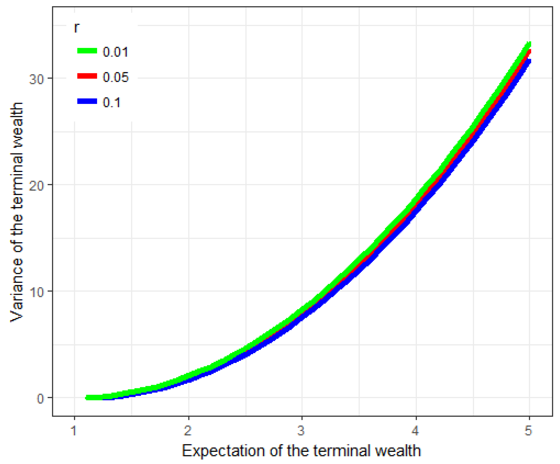
Figure 1 and Figure 2 below display the effects of r and $\lambda$ on the efficient frontier, respectively. As a matter of fact, when the interest rate r increases, the investor can obtain more expected return by investing in the risk-free asset, and thus undertake less risk. Meanwhile, from the economic implications of $\lambda$, the investor can obtain a higher risk premium of $W^1$ as $\lambda$ increases. This leads to a lower value of ${\mathrm{Var}}_{t_0,v_0,m_0,x_0}\left(X_T^{*}\right)$ when the same ${\mathrm{E}}_{t_0,v_0,m_0,x_0}\left[X_T^{*}\right]$ is asked for.

Figure 3 contributes to the evolution of the efficient frontier with respect to $l_1$. When we vary $l_1$ from $0.1$ to $0.5$, the efficient frontier moves downwards. One possible explanation is that since $l_1$ partially characterizes the liquidity term, then as $l_1$ increases, the pricing error $M_t$ in (3) has a faster mean-reversion rate towards the long-term zero such that the investor can bear less risk coming out of the pricing error between $S_1$ and $S_2$.

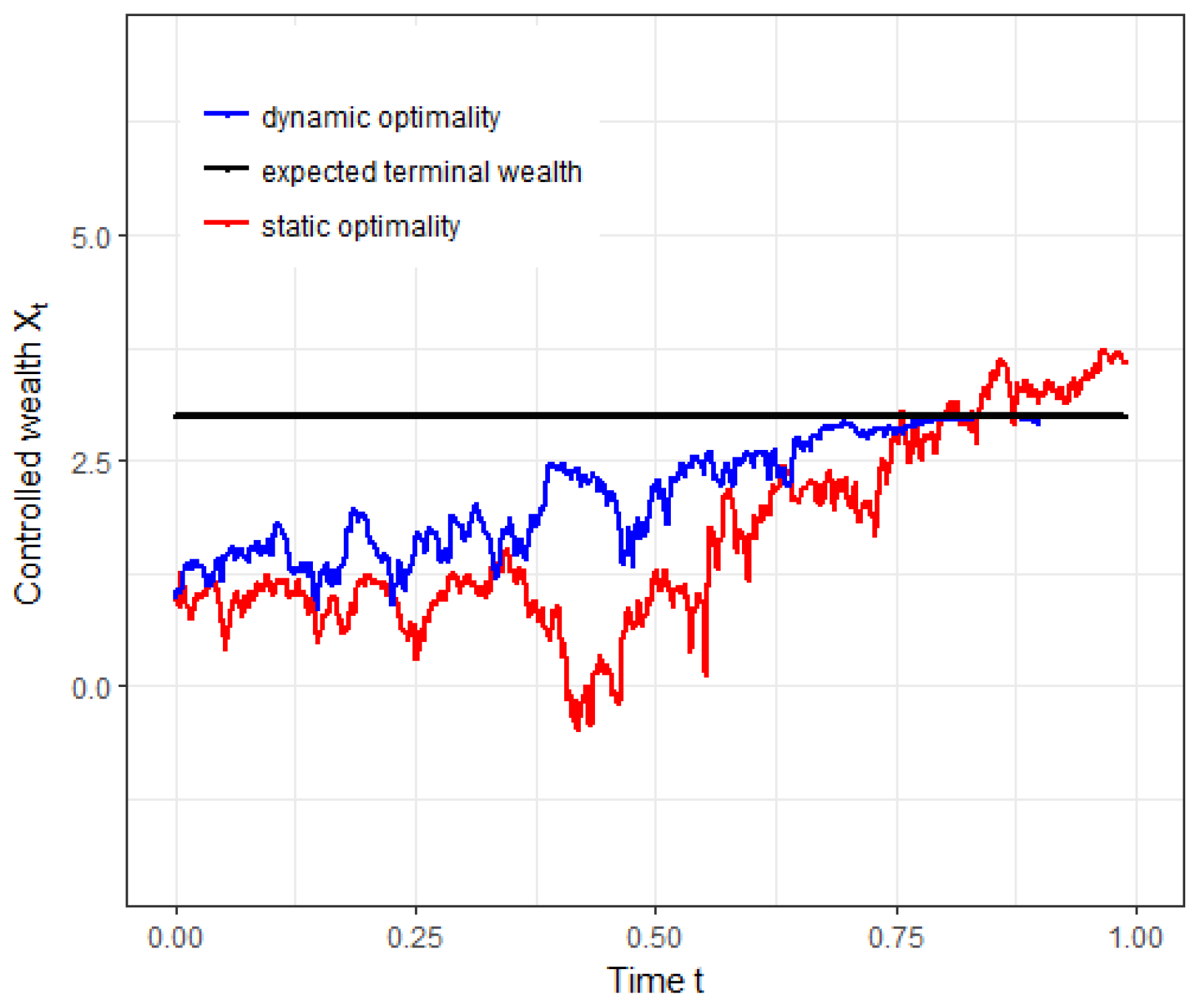
We finally give a simulation experiment to illustrate the difference between the dynamics of $X^{*}$ and $X^{d*}$. As shown in Figure 4 below, two optimal wealth processes have significantly different trajectories while using the same random numbers. Particularly, we observe that the dynamically optimal wealth process $X^{d*}$ is strictly below the expected terminal wealth $\xi =3$ when $t<T=1$ in this case, which is consistent with the conclusion derived in Theorem 3 above.

6. Conclusions

In this paper, we consider an optimal investment problem with mispricing in the family of 4/2 stochastic volatility models (Grasselli [5]) which embraces the 3/2 and the Heston models as special cases under Markowitz’s mean–variance criterion.

By applying the dynamic programming approach and establishing the corresponding HJB equation, we derive the closed-form expressions of the statically optimal (pre-commitment) strategy and the optimal value function. A verification theorem is further provided from scratch to ensure that the candidate solution to the HJB equation coincides with the optimal value function and that the optimal strategy is admissible. By recomputing the statically optimal strategy in an infinitesimally small period of time, we explicitly obtain the dynamically optimal (time-consistent) strategy (Pedersen and Peskir [24]). Moreover, some results on special cases, such as that without mispricing and that under the 3/2 and Heston models, are included. Finally, some numerical examples are presented to illustrate our results. To the best of our knowledge, there is no existing literature on the mean–variance problem with the new influential 4/2 stochastic volatility model and mispricing taken into consideration simultaneously.

Based on our current work, several potential topics in the future may be followed; for example, one may incorporate the stochastic interest rate into the model. One may also introduce random liabilities into the mean–variance problem.