On Little’s Formula in Multiphase Queues

Abstract

The structure of this work in the field of queuing theory consists of two stages. The first stage presents Little’s Law in Multiphase Systems (MSs). To obtain this result, the Strong Law of Large Numbers (SLLN)-type theorems for the most important MS probability characteristics (i.e., queue length of jobs and virtual waiting time of a job) are proven. The next stage of the work is to verify the result obtained in the first stage.

1. Introduction

Interest in the field of multiphase queueing systems has been stimulated by the theoretical values of the results, as well as by their possible applications in information and computing systems, communication networks, and automated technological processes. The investigation methods of single phase queueing systems are provided in [1,2,3]. The asymptotic analysis of queueing systems in heavy traffic models are of special interest (see, for example, in [4,5,6,7]). The papers [8,9] describe the research start of diffusion approximation relative to queueing networks. Intermediate models—multiphase queueing systems—are considered rarer due to serious technical difficulties (see, for example, book [10]).

In this paper, we present a survey of articles issued between 2010 and 2021 that investigate heavy traffic networks. In [11], a multiclass queueing system was investigated—we consider a heterogeneous queueing system to consist of one large pool of identical servers. The arriving customers belong to one of several classes, which determines the service times in the distributional sense. In [12], a class of multiclass networks was analyzed—a class of stochastic processes known as semi-martingale reflecting Brownian motions is often used to approximate the dynamics of heavily loaded queuing networks. In [13], a model of approximation of resource sharing games was developed. In [14], the problem of scheduling in queueing networks was analyzed. In [15], a model of parallel multiclass queues was investigated. The model of input queued switch operation was analyzed in [16]. In [17], the stationary distribution was investigated. The authors justified the steady-state diffusion approximation of a generalized Jackson network in heavy traffic. Their approach involves the so-called limit interchange argument, which has since become a popular tool and has been employed by many others who study diffusion approximations. A survey of stochastic network analysis was presented in [18]. In [19], MapTask scheduling in heavy traffic optimality is analyzed. In [20], the authors investigate the departure process in open queuing networks. The delay process is analyzed in [21]. Motivated by the stringent requirements on delay performance in data center networks, the authors study a connection-level model for bandwidth sharing among data transfer flows, where file sizes have phase-type distributions and proportionally fair bandwidth allocation is used. In [22], universal bounds are investigated. In [23], the load balancing policy problem in heavy traffic was developed. In [24], the MaxWeight 23 scheduling algorithm is considered. Our paper on SLLN in MS is one of the first works in this area.

The study of generalized networks can be traced back to their namesake [25,26], who considered networks with inputs and exponential service times and showed that the invariant probability for the process has a simple product form. The foregoing assumptions on the arrival streams and service times were made to greatly simplify the analysis of these networks. Relaxing these assumptions was the subject of the work by Borovkov [27], where a model similar to Markovian network is considered. The finite buffer case is treated in Konstantopoulos and Walrand [28], and general point process arrival streams and general service processes are considered for networks without feedback [29].

We will next present some definitions in the theory of metric spaces (see, for example, [30]). Let C be a metric space consisting of real continuous functions in [0, 1] with a uniform metric of the following.

$$\widehat{\rho }(m,n)=\underset{0\le s\le 1}{sup}|m\left(s\right)-n\left(s\right)|,m,n\in C.$$

Let D be a space of all real-valued right-continuous functions in [0, 1] having left limits and endowed with the Skorokhod topology, induced by the metric $\widehat{d}$ (under which D is complete and separable). Moreover, note that $\widehat{d}(m,n)\le \widehat{\rho }(m,n)$ for $m,n\in D$. In this paper, we constantly use an analog of the theorem on converging together (see, for example, [30]).

$$\begin{array}{cc}\hfill & \mathrm{Suppose}\widehat{\epsilon }>0\mathrm{and}{\mathbf{M}}_k,{\mathbf{N}}_k,\mathbf{M}\in D.If\mathbf{Pr}\left(\underset{k\to \infty }{\lim }d({\mathbf{M}}_k,\mathbf{M})>\widehat{\epsilon }\right)=0\hfill \\ \hfill & \mathrm{and}\mathbf{Pr}\left(\underset{k\to \infty }{\lim }\widehat{d}({\mathbf{M}}_k,{\mathbf{N}}_k)>\widehat{\epsilon }\right)=0,\mathrm{then}\mathbf{Pr}\left(\underset{k\to \infty }{\lim }\widehat{d}({\mathbf{N}}_k,\mathbf{M})>\widehat{\epsilon }\right)=0.\hfill \end{array}$$

(1)

There is one service device in each phase of the MS; the service discipline is FCFS (i.e., first come, first served). Service time distribution and the incoming flow of jobs to the first phase of the MS are both common. We investigate here an x-phase MS (i.e., when a job is served in the ith phase of MS, it proceeds to the $i+1$ phase of MS, and it leaves MS after the job has been served in the x-phase of MS). Let us denote the time of arrival of the kth job by $t_k$. The service time of the kth job in the ith phase of MS is denoted by $S_k^{\left(i\right)}$; $Z_k=t_{k+1}-t_k$. Let us introduce mutually independent renewal processes $m_i\left(t\right)=\{\underset{x}{max}{\displaystyle \sum _{j=1}^x}{S}_j^{\left(i\right)}\le t\}$, $e\left(t\right)=\{\underset{x}{max}{\displaystyle \sum _{j=1}^x}{Z}_j\le t\}$ (number of jobs that arrive at MS until the time moment t).

Next, we denote the number of jobs by ${\sigma }_i\left(t\right)$ after service departure from the ith phase of MS until the time t; the queue length of jobs by $Q_i\left(t\right)$ in the ith phase of MS at the time moment t; $u_i\left(t\right)={\sum }_{j=1}^i{Q}_j\left(t\right)$, $i=1,2,\dots ,x$, and $t>0$.

Let inter-arrival ($Z_k$) at MS and service times ($S_k^{\left(i\right)}$) in each phase of MS for $i=1,2,\dots ,x$ be mutually independent and identically distributed random variables.

Define ${\alpha }_i={(E{S}_k^{\left(i\right)})}^{-1}$, ${\alpha }_0={(E{Z}_k)}^{-1}$, ${\beta }_i={\alpha }_0-{\alpha }_i$, ${\beta }_0=0$, ${\hat{m}}_i\left(t\right)=e\left(t\right)-m_i\left(t\right)$, $i=1,2,\dots ,x$, $t>0$.

Suppose the following condition to be satisfied ${\alpha }_0>{\alpha }_1>\cdots >{\alpha }_x>0$. Then, the following is the case.

$${\beta }_x>{\beta }_{x-1}>\cdots {\beta }_1>0.$$

(2)

2. SLLN for the Queue Length of Jobs in MS

One of the main results of this paper is a theorem on SLLN for the summary length of jobs in MS.

Theorem 1

(SLLN for the summary length of jobs in MS). If conditions (2) are fulfilled, then the following is the case.

$$\left(\frac{V_1\left(s\right)}{s};\frac{V_2\left(s\right)}{s};\dots ;\frac{V_x\left(s\right)}{s}\right)\Rightarrow ({\beta }_1;{\beta }_2;\dots ;{\beta }_x).$$

Proof. 

The relations of the following:

$$\begin{array}{cc}\hfill Q_i\left(s\right)& ={\sigma }_{i-1}\left(s\right)-{\sigma }_i\left(s\right),\hfill \end{array}$$

(3)

$$\begin{array}{cc}\hfill Q_i\left(s\right)& =f_s({\sigma }_{i-1}(·)-m_i(·)),\hfill \end{array}$$

(4)

$$\begin{array}{cc}\hfill Q_i\left(s\right)& =f_s({\widehat{m}}_i(·)-\sum _{j=1}^{i-1}{Q}_j(·))\hfill \end{array}$$

(5)

are obtained for $i=1,2,\dots ,x$, $s>0$, and $f_s\left(m(·)\right)=m\left(s\right)-\underset{0\le p\le s}{inf}m\left(p\right)$ (see [31]).

In view of (3)–(5), we find that the following is the case:

$$v_i\left(s\right)={\widehat{m}}_i\left(s\right)-\underset{0\le p\le s}{inf}(\widehat{m}\left(p\right)-v_{i-1}\left(p\right)),$$

(6)

for $i=1,2,\dots ,x$, $s>0$.

Next, using (6) for $n_i\left(t\right)=v_i\left(t\right)-{\widehat{m}}_i\left(t\right)$, we obtain the following:

$$\begin{array}{cc}\hfill n_i\left(t\right)& \le \underset{0\le p\le t}{sup}n\left(p\right)\le \underset{0\le m\le t}{sup}(-\underset{0\le n\le m}{inf}({\widehat{m}}_i\left(n\right)-v_{i-1}\left(n\right)))\hfill \\ & =\underset{0\le p\le t}{sup}(\underset{0\le p\le m}{sup}(v_{i-1}\left(p\right)-{\widehat{m}}_i\left(p\right)))\le \underset{0\le p\le t}{sup}(v_{i-1}\left(p\right)-{\widehat{m}}_i\left(p\right))\hfill \\ & =\underset{0\le p\le t}{sup}(v_{i-1}\left(p\right)-{\widehat{m}}_{i-1}\left(p\right)+{\widehat{m}}_{i-1}\left(p\right)-{\widehat{m}}_i\left(p\right))\hfill \\ & =\underset{0\le p\le t}{sup}(n_{i-1}\left(p\right)+{\widehat{m}}_{i-1}\left(p\right)-{\widehat{m}}_i\left(p\right))\le \underset{0\le p\le t}{sup}{n}_{i-1}\left(p\right)+\underset{0\le p\le t}{sup}({\widehat{m}}_{i-1}\left(p\right)-{\widehat{m}}_i\left(p\right))\hfill \\ & \le \cdots \le \sum _{j=1}^i\underset{0\le p\le t}{sup}({\widehat{m}}_{j-1}\left(p\right)-{\widehat{m}}_j\left(p\right))\le \sum _{j=1}^x\underset{0\le p\le t}{sup}({\widehat{m}}_{j-1}\left(p\right)-{\widehat{m}}_j\left(p\right)),\hfill \end{array}$$

(7)

where $i=1,2,\dots ,x$, $t>0$.

Hence, we obtain the following:

$$v_i\left(s\right)<{\widehat{m}}_i\left(s\right)+\sum _{j=1}^x\underset{0\le p\le s}{sup}({\widehat{m}}_{j-1}\left(p\right)-{\widehat{m}}_j\left(p\right)),$$

(8)

for $i=1,\dots ,x$, $s>0$.

Thus, for any i$(i=1,2,\dots ,x)$, we obtain the following.

$$v_i\left(p\right)=\sum _{l=1}^i{Q}_l\left(p\right)=\sum _{l=1}^i[{\sigma }_{l-1}\left(p\right)-{\sigma }_l\left(p\right)]\ge e\left(p\right)-{\sigma }_l\left(p\right)\ge e\left(p\right)-m_i\left(p\right)={\widehat{m}}_i\left(p\right),$$

(9)

From (8) and (9), we obtain the following:

$$|v_i\left(s\right)-{\widehat{m}}_i\left(s\right)|\le \sum _{j=1}^x\underset{0\le p\le s}{sup}({\widehat{m}}_{j-1}\left(p\right)-{\widehat{m}}_j\left(p\right)),$$

(10)

for $i=1,\dots ,x$, $s>0$.

For $\widehat{\epsilon }>0$, we derive the following:

$$\begin{array}{cc}\hfill & Pr\left(|\frac{v_i\left(s\right)}{s}-{\hat{\beta }}_i{\displaystyle |}>\widehat{\epsilon }\right)\le Pr\left(|\frac{{\widehat{m}}_i\left(t\right)}{s}-{\widehat{\beta }}_i{\displaystyle |}>\frac{\widehat{\epsilon }}{2}\right)+Pr\left({\displaystyle |}\frac{v_i\left(s\right)-{\widehat{m}}_i\left(s\right)}{s}{\displaystyle |}>\frac{\widehat{\epsilon }}{2}\right)\hfill \\ \hfill & \le Pr\left({\displaystyle |}\frac{{\widehat{m}}_i\left(s\right)}{s}-{\widehat{\beta }}_i{\displaystyle |}>\frac{\widehat{\epsilon }}{2}\right)+\sum _{j=1}^{x}Pr\left(\frac{\underset{0\le m\le t}{sup}({\widehat{m}}_{j-1}\left(m\right)-{\widehat{m}}_j\left(m\right))}{s}>\frac{\widehat{\epsilon }}{2·x}\right),\hfill \end{array}$$

(11)

where $i=1,\dots ,x$, $s>0$.

Note that $\underset{0\le m\le s}{sup}({\widehat{m}}_{i-1}\left(m\right)-{\widehat{m}}_i\left(m\right))/s\ge 0$ for $i=1,\dots ,x$. In addition, note that the following is the case:

$$\underset{s\to \infty }{lim}\frac{{\widehat{m}}_{i-1}\left(s\right)-{\widehat{m}}_i\left(s\right)}{s}={\widehat{\beta }}_{i-1}-\widehat{\beta }{}_i<0$$

(12)

almost everywhere for $i=1,\dots ,x$ (see [31]). Thus, similarly as in [31], we prove that the second item in (11) also tends to zero.

Thus, we obtain that for $\widehat{\epsilon }>0$, the following is the case.

$$\underset{s\to \infty }{lim}Pr\left(|\frac{v_i\left(s\right)}{s}-{\widehat{\beta }}_i|>\widehat{\epsilon }\right)=0,i=1,\dots ,x.$$

(13)

Using the convergence together theorem (see, for example, [30] and (13)), we complete the proof of the theorem. □

The theorem on SLLN for the queue length of jobs is proved similarly as Theorem 1.

Theorem 2

(SLLN for the queue length of jobs in MS). If conditions (2) are fulfilled, then the following is the case.

$$\left(\frac{Q_1\left(s\right)}{s};\frac{Q_2\left(s\right)}{s};\dots ;\frac{Q_x\left(s\right)}{s}\right)\Rightarrow ({\widehat{\beta }}_1;{\widehat{\beta }}_2-{\widehat{\beta }}_1;\dots ;{\widehat{\beta }}_x-{\widehat{\beta }}_{x-1}).$$

Proof. 

Using (13), we derive the following:

$$|\frac{Q_i\left(s\right)}{s}-({\widehat{\beta }}_i-{\widehat{\beta }}_{i-1})|\le |\frac{v_i\left(s\right)}{s}-{\widehat{\beta }}_i|+|\frac{v_{i-1}\left(s\right)}{s}-{\widehat{\beta }}_{i-1}|,$$

(14)

where $i=1,\dots ,x$, $s>0$.

Using the convergence together theorem (see, for example, [30] and (14)), we complete the proof of the theorem. □

3. SLLN for the Virtual Waiting Time of a Job in MS

In this section, we present the proof of Little’s formula in MS. The main tools in proving this fact are SLLN for the queue length of jobs and the virtual length of a job in MS.

Definitions of the random variables $t_k$, $Z_k$, $S_k^{\left(i\right)}$, $e\left(t\right)$, and $m_i\left(t\right)$ for $i=1,2,\dots ,x$ are the same as in the proof of Theorems 1 and 2. Let us define ${\overline{\beta }}_i=E{S}_k^{\left(i\right)}$, ${\overline{\beta }}_0=E{Z}_k$, and ${\displaystyle {\overline{\alpha }}_i=\frac{{\overline{\beta }}_i}{{\overline{\beta }}_{i-1}}-1}$ for $i=1,2,\dots ,x$. Assume that condition (2) is fulfilled. Therefore, ${\overline{\alpha }}_i>0$ for $i=1,\dots ,x$.

In addition, let us define $V_i\left(t\right)$ as a virtual waiting time of a job in the ith phase of MS at time t. Denote $S_i\left(s\right)$ as the time, that is, the summary service of jobs arriving at the ith phase of MS until time t for $i=1,\dots ,x$ and $s>0$.

Note that $S_i\left(s\right)={\sum }_{j=1}^{{\sigma }_{i-1}\left(t\right)}{S}_j^{\left(i\right)}$ for $i=1,\dots ,x$ and $s>0$.

Moreover, let $n_i\left(s\right)=S_i\left(s\right)-s$, $f_s\left(n(·)\right)=n\left(s\right)-\underset{0\le m\le s}{inf}n\left(m\right)$, ${\widehat{n}}_i\left(s\right)={\sum }_{j=1}^{m_{i-1}\left(s\right)}{S}_j^{\left(i\right)}-s$, $m_0\left(s\right)=e\left(s\right)$ for $i=1,\dots ,x$, $s>0$.

If $S_i\left(0\right)=V_i\left(0\right)=0$, then the following is the case (see [1], p. 41).

$$V_i\left(s\right)=f_s\left(n_i(·)\right)\mathrm{for}i=1,\dots ,x\mathrm{and}s>0$$

Thus, we prove a theorem about SLLN for the virtual waiting time of a job in MS.

Theorem 3

(SLLN for the virtual waiting time of a job in MS). If conditions (2) are fulfilled, then the following is the case.

$$\left(\frac{V_1\left(s\right)}{s};\frac{V_2\left(s\right)}{s};\dots ;\frac{V_x\left(s\right)}{s}\right)\Rightarrow ({\overline{\alpha }}_1;{\overline{\alpha }}_2;\dots ;{\overline{\alpha }}_x).$$

Proof. 

Using the estimation, we obtain for each fixed $\widehat{\eta }>0$ that the following is the case:

$$\begin{array}{cc}\hfill & Pr\left(\left|\frac{V_i\left(s\right)}{s}-{\overline{\alpha }}_i\right|>\widehat{\epsilon }\right)=Pr\left(\left|\frac{f_s\left(n_i(·)\right)}{s}-{\overline{\alpha }}_i\right|>\widehat{\epsilon }\right)\hfill \\ \hfill & \le P\left(\left|\frac{f_s\left(n_i(·)\right)}{s}-\frac{f_s\left({\widehat{n}}_i(·)\right)}{s}\right|>\frac{\widehat{\epsilon }}{2}\right)+Pr\left(\left|\frac{f_s\left({\widehat{n}}_i(·)\right)}{s}-{\mu }_i\right|>\frac{\widehat{\epsilon }}{2}\right)\hfill \\ \hfill & \le Pr\left(\left|\frac{n_i\left(s\right)-{\widehat{n}}_i\left(s\right)}{s}\right|>\frac{\widehat{\epsilon }}{4}\right)+Pr\left(\left|\frac{f_s\left({\widehat{n}}_i(·)\right)-{\widehat{n}}_i\left(s\right)}{s}\right|>\frac{\widehat{\epsilon }}{4}\right)\hfill \\ \hfill & +Pr\left(\left|\frac{{\widehat{n}}_i\left(s\right)}{s}-{\overline{\alpha }}_i\right|>\frac{\widehat{\epsilon }}{4}\right)\le Pr\left(\left|\frac{n_i\left(s\right)-{\widehat{n}}_i\left(s\right)}{\sqrt{s}}\right|>\frac{\widehat{\epsilon }}{4}\right)\hfill \\ \hfill & +Pr\left(\frac{|\underset{0\le m\le s}{sup}(-{\widehat{n}}_i\left(m\right))|}{s}>\frac{\widehat{\epsilon }}{4}\right)+Pr\left(\left|\frac{{\widehat{n}}_i\left(s\right)}{s}-{\overline{\alpha }}_i\right|>\frac{\widehat{\epsilon }}{4}\right)\hfill \\ \hfill & \le Pr\left(\left|\frac{n_i\left(s\right)-{\widehat{n}}_i\left(s\right)}{\sqrt{s}}\right|>\frac{\widehat{\epsilon }}{4}\right)+Pr\left(\frac{|\underset{0\le m\le s}{sup}(-{\widehat{n}}_i\left(m\right))|}{s}>\frac{\widehat{\epsilon }}{4}\right)\hfill \\ \hfill & +Pr\left(\left|\frac{{\widehat{n}}_i\left(s\right)}{s}-{\overline{\alpha }}_i\right|>\frac{\widehat{\epsilon }}{4}\right),\hfill \end{array}$$

(15)

for $i=1,2,\dots ,x$ and $s>0$.

Thus, we achieve that for each $\widehat{\epsilon }>0$:

$$\begin{array}{c}\hfill Pr\left(\left|\frac{V_i\left(s\right)}{s}-{\overline{\alpha }}_i\right|>\widehat{\epsilon }\right)\le Pr\left(\left|\frac{n_i\left(s\right)-{\widehat{n}}_i\left(s\right)}{\sqrt{s}}\right|>\frac{\widehat{\epsilon }}{4}\right)\\ \hfill +Pr\left(\frac{|\underset{0\le m\le s}{sup}(-{\widehat{n}}_i\left(m\right))|}{s}>\frac{\widehat{\epsilon }}{4}\right)+Pr\left(\left|\frac{{\widehat{n}}_i\left(s\right)}{s}-{\overline{\alpha }}_i\right|>\frac{\widehat{\epsilon }}{4}\right),\end{array}$$

(16)

$i=1,\dots ,x$ and $s>0$.

Since it is proven ((12)), the following is the case.

$$Pr\left(\underset{s\to \infty }{lim}\left|\frac{n_i\left(s\right)-{\widehat{n}}_i\left(s\right)}{\sqrt{s}}\right|>\widehat{\epsilon }\right)=0,i=1,\dots ,x.$$

(17)

Thus, the first item in inequality (16) tends to zero (see (17)). In addition, we prove that the second item in inequality (16) also tends to zero (see, for example, [4]) (if conditions (2) are fulfilled). Therefore, we apply the limit theorem for a complex renewal process (see, for example, [5]). Thus, the third item in inequality (16) also tends to zero.

We have proven that all of the items on the inequality (16) converge to zero. Thus, we achieve that for each fixed $\widehat{\epsilon }>0$, the following is the case.

$$Pr\left(\underset{t\to \infty }{lim}\left|\frac{V_i\left(s\right)}{s}-{\overline{\alpha }}_i\right|>\widehat{\epsilon }\right)=0,i=1,\dots ,x.$$

(18)

Using the convergence together theorem (see, for example, [30] and (18)), we complete the proof of the theorem. □

Finally, we derive the corollary of proved theorems (Little’s formula). The formula L = $\lambda$W (Little’s law) expresses the fundamental principle of queueing theory: Under very general conditions, the time-average or expected time-stationary number of customers in a system, L (e.g., the average queue length), is equal to the product of the arrival rate A and the customer-average or expected customer-stationary time each customer spends in the system, W (e.g., the average waiting time). The relation L = $\lambda$W is very useful because the assumptions are minimal; it applies to other stochastic models in addition to queues; it applies to queueing networks and subnetworks as well as individual queues; it applies to subclasses as well as the entire customer population; and it is remarkably independent of modelling details, such as service disciplines and underlying probability distributions. Moreover, there are extensions of L = $\lambda$W—the continuous, distributional, ordinal and Central Limit Theorem versions, that enable us to analyze many seemingly unrelated problems.

Corollary 1

(Little’s formula in MS). If conditions (2) are fulfilled, then the following is the case.

$$\underset{s\to \infty }{lim}\frac{Q_i\left(s\right)}{V_i\left(s\right)}\Rightarrow \frac{({\widehat{\beta }}_i-{\widehat{\beta }}_{i-1})}{{\overline{\alpha }}_i},i=1,\dots ,x.$$

Proof. 

At first, we used Theorems 2 and 3 on SLLN for the queue length of jobs and virtual waiting time of a job in MS.

Thus, the following is the case.

$$\underset{s\to \infty }{lim}\frac{Q_i\left(s\right)}{V_i\left(s\right)}=\underset{s\to \infty }{lim}\frac{\frac{Q_i\left(s\right)}{s}}{\frac{V_i\left(s\right)}{s}}\Rightarrow \frac{({\widehat{\beta }}_i-{\widehat{\beta }}_{i-1})}{{\overline{\alpha }}_i},i=1,\dots ,x.$$

(19)

The proof is complete. □

4. Simulation

4.1. Overview of Similar Simulations

We have investigated many articles in order to find a similar simulation. Although we found many articles on the same topic (MS), only a few of them described the precise simulation. While investigating a similar simulation in many articles, model descriptions have been found but most of them only described the theoretical model using formulas and algorithm block schemes.

Nevertheless, a few software models or simulations have been found. The simulations that we found can be divided into two groups: (1) simulations made with particular software packages; and (2) simulations created as programs using programming languages and/or other programming tools. We can observe that these two directions of research are developing successfully (here, we can mention the recent work on modeling retrial queue systems [32,33,34], etc.).

In [35], the intelligent management system and the expert system are described. The authors describe the architecture of these systems, but no code or other details were provided. In [36], the authors apply SimEvents MATLAB-Simulink and describe the block scheme of their model. However, no programming code or details were provided.

In [37], the authors reviewed the popular simulation software, such as GPSS World, AnyLogic, and Arena environments. In the authors’ opinion, these software packages could make any simulation process very long and expensive because they are not optimal for such a simulation and are mostly used for business process simulations. In addition, most of them are commercial. Therefore, the authors decided to use their own neural network model, but no details were provided.

In [38], a real simulation model created using the Python programming language was described. The authors also provided the programming code. This simulation is described in detail, and all of the Python libraries that were used are provided.

After this review, some conclusions can be drawn:

• Commercial models do not meet the requirement to make MS simulations. In addition, they are usually expensive.
• None of the provided models meets the requirement to make all of the necessary simulations and experiments.

Consequently, we decided to create our own model that fits all of the requirements, can run on one computer and any operating system, and works in multi-threading mode.

4.2. Simulator

To implement the experiment, a Multiphase Queueing System (MS) simulator was created. The Python programming language (version 3.6.9) and its multiprocessing programming library were used. The simulator runs on any operating system that supports the Python programming language. The main new features of this simulator are the following:

• Real asynchronous processes that are not dependent on each other;
• Possibility to stop simulation at a particular time and not only when all clients are served (as [38]);
• Possibility to measure any moment of time:

  −

  Client enters MS $t_k$ (and also $Z_k=t_{k+1}-t_k$—time between two clients’ arrival);

  −

  Waiting time $V_i$ of each client in every queue;

  −

  Service time $S_{\left(i\right)k}$ of client k in the ith service of the queue;

  −

  Amount of clients $Q_i\left(t\right)$ in each queue after time t (when the process stopped after time t);

• Client proceeds to the consumer process not only after it pass all services (as [38]) but also immediately if MS stopped after the specified time t;
• All of the values to be measured are stored in synchronized variables for eliminating their undefined states (some issues could appear because of the operating system, the Python programming language, or hardware errors);
• Each service really stops after all of the clients pass away or after the specified time t;
• Clients enters the consumer process from any place of MS if it stops after the specified time t. For example, a client cannot pass all of the services or could even be in a waiting queue for one of the services;
• All of the calculations are performed, and only then is MS stopped or when all the clients pass through or after the specified time ends.

As shown in Figure 1, the simulator has input (producer process) and output (consumers process) storage and I (configurable) phases in the queue between them. K (configurable) clients created by producer process with random (configurable) time interval between them proceed to the first phase and then, after they have been served there, they proceed to the next phase. Each phase has its own serving time and waiting time before serve. The process continues until the last queue is stopped, after which the client comes to the consumer process.

The main difference in this model is the possibility to stop the simulation after a particular time t (configurable) interval. Imagine that somebody wants to stop the simulation after time t. Then, after the specified time, all of the phases are stopped in the state that they are in and the consumer process collects all of the clients from all of the phases. Here, all the calculations could be performed, including client number in the phase at the moment t.

In this simulation, when it finishes after the specified time t, all clients have their own states and other information, such as the following:

• All times between jobs’ arrivals to MS;
• All service times of all jobs in all queues (where they had time to gain);
• All jobs waiting times in all queues and the number of jobs in all queues at time t (when the simulation stopped).

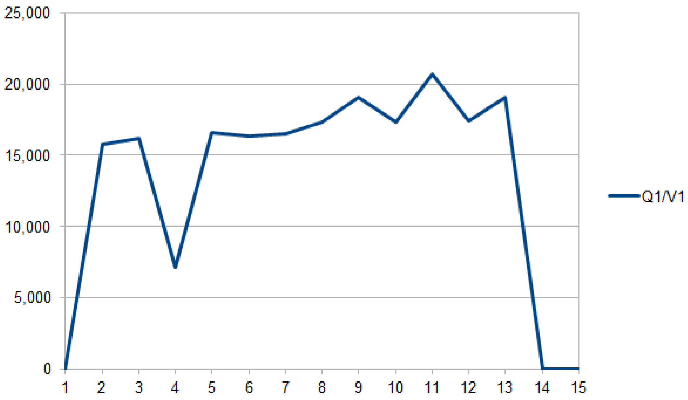
All of the measurable parameters of the model are listed in

Table 1. Model parameters.

Parameter	Description
$t_k$	Client’s k arrival to MS time
$V_i$	Client’s waiting time before service in the ith phase
$S_i$	Client’s service time in the ith phase
$Q_i$	Clients amount in the ith phase at the moment t

.

After the model stops, the consumer process performs all of the computations for the values listed in

Table 2. Computational parameters of the model.

Parameter	Description
$E\left(V_i\right)$	Estimated waiting time before service in the ith phase
$E\left(S_i\right)$	Estimated service time in the ith phase
$Q_i/t$	Clients amount in the queue i at time t, divided by t
$Z_{k+1}$	Estimated time between two clients entering MS
$E\left(Z\right)$	Estimated time between clients on entering MS

.

4.3. Experiment

The experiment results were obtained using this simulation with the following parameters:

• Time interval of 15 s (measurements were made each second from 1 to 15);
• Five phases in MS;
• 100,000 clients received from the producer.

During the experiment, the MS system was stopped at each second, and all of the calculations were made. In each phase, the following is the case:

• $Q_1$–$Q_5$—numbers of clients in all five phases divided by t;
• $E\left(V_1\right)$–$E\left(V_5\right)$—estimated waiting times in each phase are calculated and divided by t;
• $Q_1/V_1$–$Q_5/V_5$ ratios for each phase are calculated.

The list of hardware and software used in the experiment is provided in

Table 3. Hardware and software used in the experiment.

OS	Linux Mint, Linux PC 5.4.0-62-generic #70-Ubuntu SMP Tue Jan 12 12:45:47 UTC 2021 ×86_64 ×86_64 ×86_64 GNU/Linux
Python programming language	Python 3.6.9 (default, 18 April 2020, 01:56:04) [GCC 8.4.0] on Linux
Python libraries	multiprocessing, time, random, numpy, sys, asyncio, matplotlib, pylab, matplotlib.pyplot, math, ctypes
IDE	Visual Studio Code
Processor	Intel(R) Core(TM) i7-8700 CPU @ 3.20 GHz
Memory	32747MB (17387MB used)
Storage	ATA Samsung SSD 860
Video adapter	NVIDIA GeForce GTX 1080 Ti/PCIe/SSE2

.

The results of calculation ratios $Q_1/V_1$, $Q_2/V_2$, $Q_3/V_3$, $Q_4/V_4$, and $Q_5/V_5$ in 1–15 s simulations are provided in

Table 4. Results of ratio calculation.

t, s	${\mathit{Q}}_1/{\mathit{V}}_1$	${\mathit{Q}}_2/{\mathit{V}}_2$	${\mathit{Q}}_3/{\mathit{V}}_3$	${\mathit{Q}}_4/{\mathit{V}}_4$	${\mathit{Q}}_5/{\mathit{V}}_5$
1	0	0	0	0	0
2	15,783.208889	7713.886687	10,173.894957	8327.816417	4849.444553
3	16,158.595911	24,539.397682	3903.148301	12,644.343116	7150.621767
4	7150.621767	14,994.150418	4764.470185	9563.342329	9489.530662
5	16,618.375117	11,304.161697	24,609.465659	11,133.676329	7467.462789
6	16,349.095476	16,200.135701	10,906.525734	21,445.316714	7687.643707
7	16,540.717478	10,413.616874	17,795.190157	11,758.146436	9688.644638
8	17,363.635526	11,608.885913	13,812.022670	14,145.828118	8471.549574
9	19,027.493286	15,717.070406	19,310.638918	13,772.830493	14,585.097103
10	17,339.523710	11,679.801550	14,368.463078	12,014.946867	10,045.985695
11	20,742.679577	23,891.867419	15,796.962250	17,233.303617	18,584.620158
12	17,426.702838	84,383.182448	12,677.306401	11,978.191479	8637.416323
13	19,019.020194	16,494.458220	21,366.420617	20,901.589822	26,116.328410
14	0	0	0	0	0
15	0	0	0	0	0

.

The ratios mentioned in Table 4 are provided in Figure 2, Figure 3, Figure 4, Figure 5 and Figure 6, respectively.

4.4. Description of the Results

As described in the theory, each $Q_i/E\left(V_i\right)$ ratio should converge into a constant. This was an expected result—each $Q_i/E\left(V_i\right)$ ratio after some period of time converges into a constant value or becomes almost stable after some period of time and remains fairly stable for a certain period of time. In the theory, we have an infinite flow of clients, really independent phases, and infinitely large computational resources. In other words, we really have the ideal conditions and no faults or errors.

In reality, this model runs on one computer where there is one processor with real and virtual cores, memory, and storage limits. Under these conditions, some unstable work of the system is present because it is impossible to eliminate all of the faults and errors. A more important point is that the computer’s operating system shares resources between processes using its own algorithms, and it can be difficult to allocate the required amount of hardware resources to a particular process.

Another significant problem is the lack of resources, which produces some limitation for any model work (e.g., to have an infinite flow of jobs). Each phase could also be “clogged” with clients when another one is waiting for them. In addition, during the experiment, other restrictions appeared in the current configuration. For example, in theory we need to use the infinite number of clients, but in reality using even 1,000,000 is difficult.

In the real condition, there are some faults and errors in multi-threading libraries when using the Python programming language, and there are some undefined states. Some other mistakes could appear due to the calculation accuracy and time measurement because approximations are used. The lack of resources especially affects measurements of time because the system could lag.

The most expected result is to find a stable interval for every phase where the equilibrium of model load and theoretical conditions are satisfied and to create the experiment where all listed theorems could be checked. A stable time interval should be found for each ratio, in this interval the ratio of $Q_j/E\left(V_j\right)$ should be the same or very similar.

All of the calculation results for each ratio are listed above. In every chart of each ratio, we can observe the state and the time when the ratio becomes stable or changes a little. Each phase becomes a stable state at a different time period. This could happen because of different times of the critical load and also because of no load for each phase.

For example, the first ratio $Q_1/E\left(V_1\right)$ becomes stable after 2 s (4 s value is an issue) and remains stable until 13 s. The second ratio is more stable from 3 to 11 s, the third from 6 to 12, the fourth from 7 to 12, and the fifth is more stable at the beginning but less stable at the end. It is difficult to find a stable period for the fifth (or last) phase because it becomes clogged after all of the other phases are empty or almost empty. When a large flow of clients arrives, the period of stability should begin, but the phase becomes empty very soon. In addition, for this configuration, all clients pass MS at the 14^th second, and all phases become empty.

This experiment result shows that each phase has its own stability period; thus, it could be considered that the ratio of $Q_j/E\left(V_j\right)$ converges to a constant, as proved in the theory.

Corollary 2

(Validation of Little’s formula in MS). At this stage of the work, we confirm that the results of the first stage are correct.

5. Concluding Remarks

• We observe that the heavy traffic condition used in the proof of the theorems on SLLN is fundamental. Abandoning this condition makes the proof of the theorems very complicated. In the future, it would be interesting to examine the situation under light traffic.
• By using another method to prove theorems and normalizing boundary processes differently than compared to SLLN (e.g., probability limit theorems or the law of the iterated logarithm—but this is implicated only in the single-phase case, and there is no research in the multiphase case), Little’s law becomes the successful process or becomes its law of the iterated logarithm analog. With SLLN, the boundary process is constant—this process can be modeled.
• The theoretical results cannot be directly verified by modeling them, which is evidenced by the modeling block diagram. Modeling has its own explicit specifics; thus, a comprehensive review of the literature in this area was required.
• The ideas of the modeling part are related to the often cited work [38]. In this work, for the first time, the modern possibilities of the Python programming language were applied in order to model the queuing system. Continuing this topic, the Python concept was used to test the theoretical results of the first stage.
• The first and second parts of this paper deal with similar but completely separate subject areas. As much as possible, efforts were made to bring them closer together and to present them as a single study.

References

1. Borovkov, A. Stochastic Processes in Queueing Theory; Nauka: Moscow, Russia, 1972. (In Russian) [Google Scholar]
2. Borovkov, A. Asymptotic Methods in Theory of Queues; Nauka: Moscow, Russia, 1980. (In Russian) [Google Scholar]
3. Saati, T.; Kerns, K. Analytic Planning. Organization of Systems; Mir: Moscow, Russia, 1971. (In Russian) [Google Scholar]
4. Iglehart, D.L.; Whitt, W. Multiple channel queues in heavy traffic. I. Adv. Appl. Probab. 1970, 2, 150–177. [Google Scholar] [CrossRef]
5. Iglehart, D.L.; Whitt, W. Multiple channel queues in heavy traffic. II: Sequences, networks and batches. Adv. Appl. Probab. 1970, 2, 355–369. [Google Scholar] [CrossRef]
6. Kingman, J. On queues in heavy traffic. J. R. Stat. Soc. Ser. (Methodol.) 1962, 24, 383–392. [Google Scholar] [CrossRef]
7. Kingman, J. The single server queue in heavy traffic. Math. Proc. Camb. Philos. Soc. 1961, 57, 902–904. [Google Scholar] [CrossRef]
8. Kobyashi, H. Application of the diffusion approximation to queueing networks I: Equilibrium queue distributions. J. ACM 1974, 21, 316–328. [Google Scholar] [CrossRef]
9. Reiman, M.I. Open queueing networks in heavy traffic. Math. Oper. Res. 1984, 9, 441–458. [Google Scholar] [CrossRef]
10. Karpelevich, F.I.; Kreinin, A.I. Heavy traffic limits for multiphase queues. Transl. Math. Monogr. 1994, 137. [Google Scholar] [CrossRef]
11. Gamarnik, D.; Stolyar, A.L. Multiclass multi-server queueing system in the Halfin-Whitt heavy traffic regime: Asymptotics of the stationary distribution. Queueing Syst. 2012, 71, 25–51. [Google Scholar] [CrossRef] [Green Version]
12. Gurvich, I. Validity of heavy-traffic steady-state approximations in multiclass queueing networks: The case of queue-ratio disciplines. Math. Oper. Res. 2014, 39, 121–162. [Google Scholar] [CrossRef]
13. Wu, Y.; Bui, L.; Johari, R. Heavy traffic approximation of equilibria in resource sharing games. Internet Netw. Econ. 2011, 351–362. [Google Scholar] [CrossRef] [Green Version]
14. Markakis, M.G.; Modiano, E.; Tsitsiklis, J.N. Max-weight scheduling in queueing networks with heavy-tailed traffic. IEEE/ACM Trans. Netw. 2014, 22, 257–270. [Google Scholar] [CrossRef] [Green Version]
15. Anselmi, J.; Casale, G. Heavy-traffic revenue maximization in parallel multiclass queues. Perform. Eval. 2013, 70, 806–821. [Google Scholar] [CrossRef] [Green Version]
16. Maguluri, S.T.; Burle, S.K.; Srikant, R. Optimal heavy-traffic queue length scaling in an incompletely saturated switch. Queueing Syst. 2018, 88, 279–309. [Google Scholar] [CrossRef] [Green Version]
17. Braverman, A.; Dai, J.G.; Miyazawa, M. Heavy traffic approximation for the stationary distribution of a generalized Jackson network: The BAR approach. Stochastic Syst. 2017, 7, 143–196. [Google Scholar] [CrossRef]
18. Butler, R.W.; Huzurbazar, A.V. Stochastic Network Models for Survival Analysis. J. Am. Stat. Assoc. 1997, 92, 246–257. [Google Scholar] [CrossRef]
19. Wang, W.; Zhu, K.; Ying, L.; Tan, J.; Zhang, L. MapTask scheduling in mapreduce with data locality: Throughput and heavy-traffic optimality. IEEE/ACM Trans. Netw. 2016, 24, 190–203. [Google Scholar] [CrossRef]
20. Whitt, W. Some useful functions for functional limit theorems. Math. Oper. Res. 1980, 5, 67–85. [Google Scholar] [CrossRef] [Green Version]
21. Wang, W.; Maguluri, S.T.; Srikant, R.; Ying, L. Heavy-traffic delay insensitivity in connection-level models of data transfer with proportionally fair bandwidth sharing. ACM Sigmetrics Perform. Eval. Rev. 2017, 45, 232–245. [Google Scholar] [CrossRef]
22. Huang, J.; Gurvich, I. Beyond heavy-traffic regimes: Universal bounds and controls for the single-server queue. Oper. Res. 2018, 66, 1168–1188. [Google Scholar] [CrossRef]
23. Zhou, X.; Tan, J.; Shroff, N. Flexible load balancing with multidimensional state-space collapse: Throughput and heavy-traffic delay optimality. Perform. Eval. 2018, 127–128, 176–193. [Google Scholar] [CrossRef] [Green Version]
24. Maguluri, S.T.; Srikant, R. Heavy traffic queue length behavior in a switch under the MaxWeight algorithm. Stoch. Syst. 2016, 6, 211–250. [Google Scholar] [CrossRef]
25. Jackson, J.R. Jobshop-like queueing systems. Manag. Sci. 1963, 10, 131–142. [Google Scholar] [CrossRef]
26. Kelly, F.P. Reversibility and Stochastic Networks; Wiley: New York, NY, USA, 1987. [Google Scholar]
27. Borovkov, A.A. Limit theorems for queueing networks. I. Theory Probab. Its Appl. 1987, 31, 413–427. [Google Scholar] [CrossRef]
28. Konstantopoulps, P.; Walrand, J. On the ergodicity of networks of ·/GI/1/N queues. Adv. Appl. Probab. 1990, 22, 263–267. [Google Scholar] [CrossRef] [Green Version]
29. Konstantopoulps, P.; Walrand, J. Stationarity and stability of fork-join networks. J. Appl. Probab. 1989, 26, 604–614. [Google Scholar] [CrossRef]
30. Billingsley, P. Convergence of Probability Measures; Wiley: New York, NY, USA, 1968. [Google Scholar]
31. Minkevičius, S. Weak convergence in multiphase queues. Lith. Math. J. 1986, 26, 347–351. [Google Scholar] [CrossRef]
32. Melikov, A.; Aliyeva, S.; Sztrik, J. Analysis of Instantaneous Feedback Queue with Heterogeneous Servers. Mathematics 2020, 8, 2186. [Google Scholar] [CrossRef]
33. Sztrick, J.; Toth, A.; Pinter, A.; Bacs, Z. Reliability Analysis of Finite-Source Retrial Queueing Systems with Two-Way Communications to the Orbit and Blocking Using Simulation. In Proceedings of the 23rd International Scientific Conference on Distributed Computer and Communication Networks: Control, Computation, Communications (DCCN-2020), Moscow, Russia, 14–18 September 2020; pp. 260–267. [Google Scholar]
34. Sztrik, J.; Tóth, Á.; Pintér, Á.; Bács, Z. The simulation of finite-source retrial queueing systems with two-way communications to the orbit and blocking. In International Conference on Distributed Computer and Communication Networks; Springer: Cham, Switzerland, 2020; pp. 171–182. [Google Scholar] [CrossRef]
35. Bychkov, I.V.; Kazakov, A.L.; Lempert, A.A.; Bukharov, D.S.; Stolbov, A.B. An intelligent management system for the development of a regional transport logistics infrastructure. Autom. Remote Control 2016, 77, 332–343. [Google Scholar] [CrossRef]
36. Harahap, E.; Darmawan, D.; Fajar, Y.; Ceha, R.; Rachmiatie, A. Modeling and simulation of queue waiting time at traffic light intersection. J. Phys. Conf. Ser. 2019, 1188, 012001. [Google Scholar] [CrossRef]
37. Gorbunova, A.V.; Vishnevsky, V.M.; Larionov, A.A. Evaluation of the end-to-end delay of a multiphase queuing system using artificial neural networks. In International Conference on Distributed Computer and Communication Networks; Lecture Notes in Computer Science; Springer: Cham, Switzerland, 2020; pp. 631–642. [Google Scholar] [CrossRef]
38. Dolgopolovas, V.; Dagienė, V.; Minkevičius, S.; Sakalauskas, L. Python for scientific computing education: Modeling of queueing systems. Sci. Program. 2014, 22, 37–51. [Google Scholar] [CrossRef]
Figure 1. Algorithm of the simulation model.
Mathematics 09 02282 g001
Figure 2. Ratio of Q 1 / V 1 .
Mathematics 09 02282 g002
Figure 3. Ratio of Q 2 / V 2 .
Mathematics 09 02282 g003
Figure 4. Ratio of Q 3 / V 3 .
Mathematics 09 02282 g004
Figure 5. Ratio of Q 4 / V 4 .
Mathematics 09 02282 g005
Figure 6. Ratio of Q 5 / V 5 .
Mathematics 09 02282 g006