A Learning-Based Hybrid Framework for Dynamic Balancing of Exploration-Exploitation: Combining Regression Analysis and Metaheuristics

Abstract

The idea of hybrid approaches have become a powerful strategy for tackling several complex optimisation problems. In this regard, the present work is concerned with contributing with a novel optimisation framework, named learning-based linear balancer ($L{B}^2$). A regression model is designed, with the objective to predict better movements for the approach and improve the performance. The main idea is to balance the intensification and diversification performed by the hybrid model in an online-fashion. In this paper, we employ movement operators of a spotted hyena optimiser, a modern algorithm which has proved to yield good results in the literature. In order to test the performance of our hybrid approach, we solve 15 benchmark functions, composed of unimodal, multimodal, and mutimodal functions with fixed dimension. Additionally, regarding the competitiveness, we carry out a comparison against state-of-the-art algorithms, and the sequential parameter optimisation procedure, which is part of multiple successful tuning methods proposed in the literature. Finally, we compare against the traditional implementation of a spotted hyena optimiser and a neural network approach, the respective statistical analysis is carried out. We illustrate experimental results, where we obtain interesting performance and robustness, which allows us to conclude that our hybrid approach is a competitive alternative in the optimisation field.

1. Introduction

In recent years, the constant increase in complexity of the problems to be solved in the industry and academy have raised the necessity to further improve and evolve new techniques. In this context, hybrid approaches have been a standard and focus of multiple works. They have proved to be the most successful strategy in terms of solving capacity tackling hard optimisation problems [1]. In modern approaches, the use of randomised optimisation methods have been the focus of work by the scientist community, a well-known example are the metaheuristics. They have been successfully used to solve large instance of complex and difficult optimisation problems, being useful when exact methods are unable to provide solutions in a reasonable amount of time [2]. Usually, in the design behind an algorithm, we find multiple complex items which are in charge of carrying out the work in order to solve optimisation problems [3]. Inherent features, like intensification and diversification [4,5,6], which are in control on how the approach can exploit and explore the search space, respectively. Additionally, parameters and search components, such as population, probabilities, search operators, initial solutions, and so on, comprehend important family items in the work of an approach. In order to be intelligent, an agent which works in a changing environment should have the ability to learn [7]. If the approach can learn and adapt, we do not need to foresee and provide solutions for all possible situations which may appear on run-time. Machine learning, being part of artificial intelligence, encircle a number of algorithms with the aim to optimise a performance criterion using example data or past experience [8,9,10]. A well-known style of learning is the supervised learning, which is mainly composed by learning functions with the aim of predict values, and some of his classical objectives are regression and classification [11].

In this paper, we examine whether a formal relationship between an effective balance of intensification and diversification, influenced by a regression model, and a classic configuration of a metaheuristic exists, and whether it is sufficiently strong to be exploited for an automated framework. Most metaheuristics operate in a sequential, iterative, and in a previously designed manner, but the environment where they operate usually has a dynamic nature. Additionally, they are stochastic algorithms, which comprehends deterministic and random components. The stochastic components can take many forms, such as simple randomisation by randomly sampling the search space or by random walks. Thus, the randomness brings certain degree of uncertainness in the search. For instance, if an agent just finished performing an intensification movement, and the next step in the process performs a diversification movement, it has no certainty on reaching a better neighbourhood. In Figure 1, we illustrate a graphic example of a situation where a white agent needs to make a move; we aim to help the agent to have higher possibility to reach a green dot (possible best solution) or a yellow dot (less possible best solution) than a red dot (bad solution). The objective in the design of this framework is to let the approach learn how to orchestrate the work performed by the agents in every iteration, hence, we enforce the decision making of the approach and make him learn from previous iterations on run-time. In this regard, two components are designed: movements operators; in this work we employ movements from the spotted hyena optimiser (SHO) algorithm [12], and a regression model. First, SHO is an interesting modern metaheuristic, which has proved to yield good results in solving optimisation problems [13,14]. It is mainly based in the grouping behaviours of a special type of Hyena, where the strong point in the algorithm is the clustering features of the agents searching in the solution space. On the other hand, the learning model, is where the central axis of the work is completed by linear regression analysis. The work is completed as follows: dynamic data generated by the agents through iterations will be managed by the learning model. In this context, each time a threshold amount of iteration is met, a regression analysis is carried out by the learning model. Thus, the search will be influenced by the resulting knowledge from the previous learning process.

The efficiency of $L{B}^2$ proposed in this research is evaluated in three phases by solving 15 well-known mathematical optimisation problems. The employed benchmark concerns unimodal, multimodal, and mutimodal functions with fixed dimension. Additionally, these continuous functions comprehends multiple features, such as being convex, non-differentiable, unconstrained, and so on. Regarding the experimentation phases, we compare our results with state-of-the-art optimisation methods, such as particle swarm optimisation (PSO) [15], gravitational search algorithm (GSA) [16], differential evolution (DE) [17], whale optimisation algorithm (WOA) [18], vapour–liquid equilibrium (VLE) [19], and an hybrid between Nelder–Mead algorithm and dragonfly algorithm (INMDA) [20]. In the second phase, we compare against sequential parameter optimisation (SPO) [21]. The key work in SPO is performed by a prediction model, bringing improvements in the parameters values and algorithm performance in an iterative scheme. Third, we carry out a statistical evaluation of the results obtained by the traditional implementation of SHO, neural network (NN) [22], sine cosine algorithm (SCA) [23], and our proposed hybrid approach. Finally, we illustrate interesting experimental results, where the proposed hybrid approach achieves good performance proving to be a good and competitive option to tackle continuous optimisation problems.

The rest of this paper is organised as follows. The related work is introduced in the next section. The proposed hybrid approach is explained in Section 3. Section 4 illustrates the experimental results. Finally, we conclude and suggest some lines of future research.

2. Related Work

This work proposes a learning-based hybrid approach, where the main feature is the capability to influence the search performed by the agents ruled by the movements of SHO. Therefore, following the taxonomy illustrated by Talbi in [24], our proposed work can be described as a low-level teamwork hybridisation. Concerning the works reported in the literature between machine learning and metaheuristics [8,25], it is well-known that this relationship is not a one-way street, we do not have only approaches were machine learning techniques assist and enhance metaheuristics, but also the other way around: machine learning models improved by metaheuristics, is a much consolidated group in the hybridisation field [26,27,28,29,30]. This paper is concerned with the first group, where novel approaches have been proposed, such as [31], where a diversification-based learning (DBL) framework is proposed. DBL is designed under families of components introduced in the field of metaheuristics and machine learning that have broad applications in optimisation. Additionally, a novel approach based on two well-known components is presented in [32], an hybrid between intelligent guided adaptive search (IGAS) and path-relinking algorithm, named IGASPR. The main learning phase is ruled by the means of growing neural gas (GNG), the objective is to influence the construction of solutions controlling the features of the best solutions in each iteration. Concerning proposed works under the influence of regression analysis, [33] illustrates a data mining based approach for PSO. The main ideas behind that contribution is that the parameter selection task can appropriately be addressed by a data mining-based approach. The designed model employs a regression analysis by means of non-linear regression models, the main objective is to learn suitable parameters values from previous moves for PSO on run-time. In this field, this type of scheme is also known as specifically-located hybridisation and it is concerned with the parameter control strategies. In the literature, [34] also employ this type of hybridisation. The authors propose an hybrid employing Tabu search (TS) and support vector machine (SVM). The proposed approach is designed to tackle on hard combinatorial optimisation problems, such as knapsack problem, set covering problem, and the travelling salesman problem. The main task concerns the selection of decision rules from a corpus of solutions generated in a randomly fashion, which are used to predict high quality solutions for a given instance and it is used to fine-tune and guide the search performed by TS. However, it is stated by the authors that the complexity of the approach is a key factor, they highlight the time consumed and knowledge necessarily needed to implement, the process to build the corpus, and the extraction of the classification rule. On the other hand, regarding hybrid specialising in intensification and diversification, to the best of our knowledge there was none under the influence of a regression model. However, in [25], the feasible options on intensification employing clustering [35] and frequent itemsets using association rules [36,37] are illustrated. Regarding diversification, the use of clustering [35], self-organising maps (SOM) [38], and binary space-partitioning (BSP) trees [39] have proved to be good options balancing this issue in different approaches.

The $L{B}^2$ proposed in this work draws inspiration by the following arguments. Firstly, the scarce literature concerning machine learning mainly associated to regression model assisting metaheuristics. Second, most approaches are problem-dependant, for instance, in [32], the problem to be tackled by the regression model is the selection of best fitted parameters for PSO in order to improve the performance. It is a good exploratory and pioneer approach considering this attempt to be on run-time. However, the uncertainty in extrapolating this specifically-located implementation to other approaches is high, especially taking into account the “no free lunch” theorem. Therefore, our proposition focus in two major issues when designing a global search method, diversification, and intensification. Thus, if we analyse the metaheuristic field, they are general features who are always present. Third, the technique selected is a highly relevant issue. It is stated and explained by authors, in [33], the level of complexity is an issue to take into account in the design of the hybrid. Thus, we think this issue may have an impact replicating the results and extrapolating the implementation to an unknown environment. In this context, we employ classic techniques, where the novel mechanism are the clear advantages provided by our proposed hybrid approach.

3. Proposed Hybrid Approach

In this section we present the proposed $L{B}^2$ framework, we discuss the main ideas in the design, motivations, and inspiration behind the proposed approach. Firstly, in order to carry out the search in the solution space, the strategy employed is inspired by population-based metaheuristics. The main idea is to perform using a set of agents who evolve under the influence of multiple equations, known as movement of operators. In this regard, they are usually classified as intensification and diversification concerning the work performed, exploitation or exploration of the search space. In this work we employ SHO and his four movement operators, where each hyena is currently an agent in the framework.

The second answer proposed is concerned with the component in charge of the regression analysis. In this first attempt to design $L{B}^2$ the main concern was the complexity of the employed technique [40,41]. In this regard, multiple techniques and methods to carry out a regression analysis [42], such as linear models, SVM, and decision-tree-based models. Thus, a linear model was selected because it is the most commonly used, and all other regression methods build upon an understanding on how linear regression works [43,44]. Nevertheless, the regression model can potentially evolve in a more complex component, a more detailed explanation is presented in Section 5.

The global conceptualisation of the proposed hybrid is illustrated in Figure 2. It is based in the behaviour of multiple agents with the same attributes, also known as population. They are controlled by the movements of SHO, influenced and balanced by the learning-based model. A general description is presented in Section 3.1. The methodology and detailed explanation of the proposed approach is explained in Section 3.2. In Section 3.3, the population-based metaheuristic is presented, and the proposed algorithm is illustrated in Section 3.4.

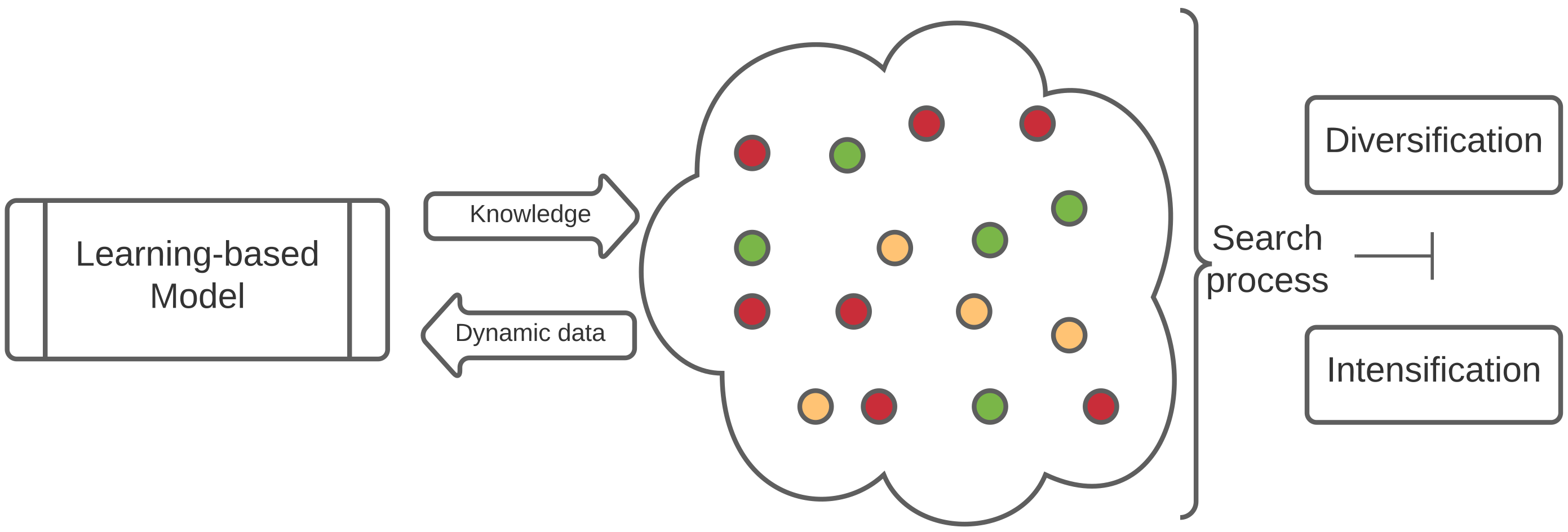
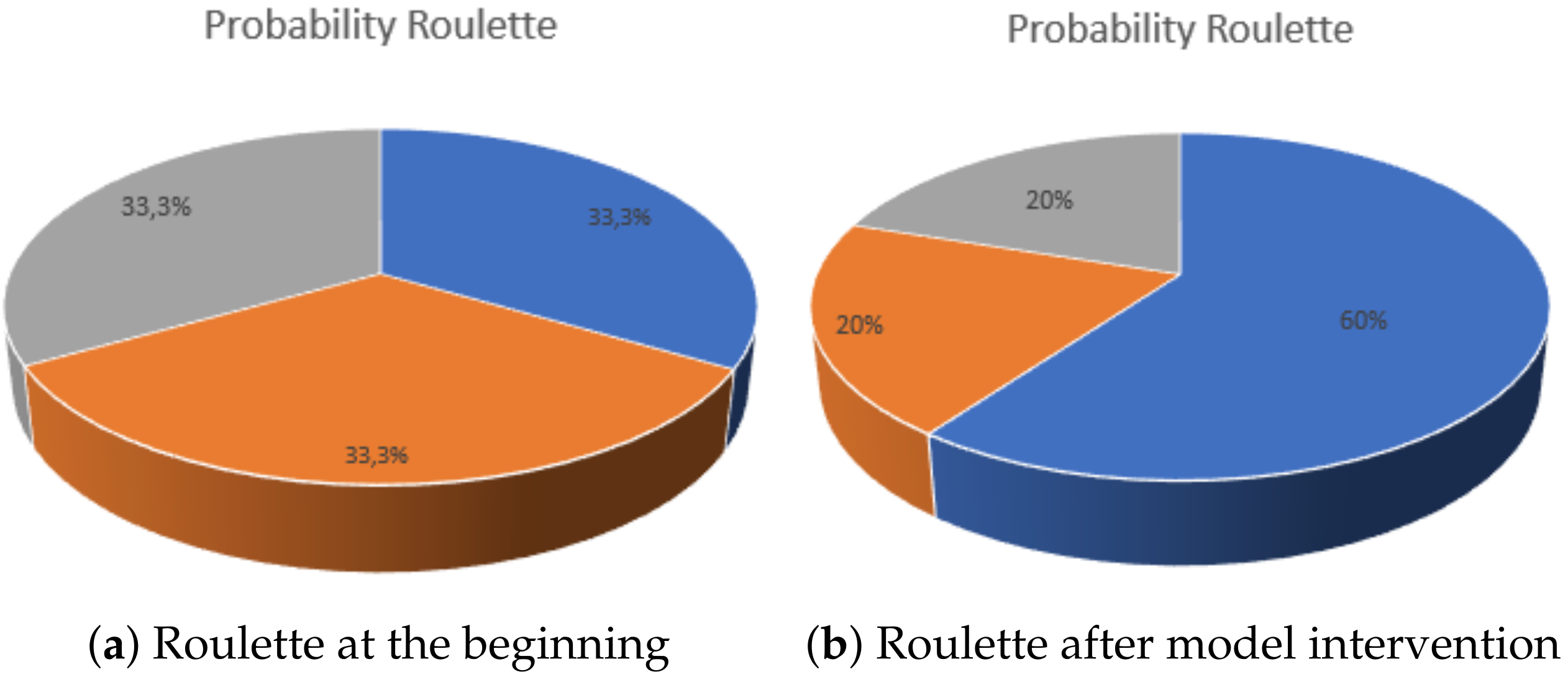
3.1. General Description

The proposed $L{B}^2$ follows a population-based strategy, which concerns multiple agents evolving in the solution space, intensification and diversification are performed, and the process is terminated when a threshold amount of iteration is met. Dynamically adjusting the configuration and behaviour is an important topic that continues to be of growing interest. This work, in order to carry out the search, proposes two components: scheme and $\beta$. Firstly, the scheme is concerned with the amount of intensification and diversification to be performed in each iteration by the population. Regarding $\beta$, it is a parameter employed as the threshold where the learning model needs to carry out the regression analysis. The knowledge generated will be used to influence the selection mechanism, which manages the scheme that needs to be performed. In this regard, the selection will dynamically rule over the work of each agent, indicating the amount of exploration and exploitation to carry out in the search space. The proposed steps of the proposed $L{B}^2$ are described as follows:  

Step 1: Set parameters concerning the population-based algorithm: B,E,h, termination criteria for the search.

Step 1.1: Set termination criteria for the search: set amount of iterations to perform $L{B}^2$.

Step 2: Set parameters concerning the learning model: scheme, probabilities, $\beta$.

Step 2.1: Set schemes for intensification and diversification.

Step 2.2: Set the probabilities for each scheme to be selected by the selection mechanism.

Step 2.3: Set the value for threshold $\beta$.

Step 3: Generation of the initial population size to perform in the search.

Step 4: while the termination criteria is not met.

Step 5: For each agent:

Step 5.1: Selection mechanism on intensification: the scheme is selected and the exploitation is carried out.

Step 5.2: Management of dynamic data generated.

Step 5.3: Selection mechanism on diversification: the scheme is selected and the exploration is carried out.

Step 5.4: Management of dynamic data generated.

Step 6: Update parameters concerning the population-based algorithm: B,E,h.

Step 7: Check if the threshold $\beta$ has been met.

Step 7.1: Perform regression analysis.

Step 7.2: Management of the knowledge generated: update scheme probabilities.

3.2. Methodology

Firstly, we need to define the schemes to perform through the search, in this first attempt designing $L{B}^2$, three levels where proposed and illustrated in

Table 1. Example of the standard work to be completed by the approach.

Scheme	Amount of Intensification	Amount of Diversification
Soft	1	1
Medium	2	2
Hard	3	3

. They define the amount of work that needs to be performed in each iteration, the selection issue is tackled by the means of probabilities, and they are defined as follows.

$$\mathrm{for}\mathrm{intensification}:p_i=\frac{1}{{\mathrm{IS}}_{\mathrm{soft}}}+\frac{1}{{\mathrm{IS}}_{\mathrm{medium}}}+\frac{1}{{\mathrm{IS}}_{\mathrm{hard}}}=1$$

$$\mathrm{for}\mathrm{diversification}:p_d=\frac{1}{{\mathrm{DS}}_{\mathrm{soft}}}+\frac{1}{{\mathrm{DS}}_{\mathrm{medium}}}+\frac{1}{{\mathrm{DS}}_{\mathrm{hard}}}=1$$

where the probability $p_i$ and $p_d$ will be modified by the learning model every $\beta$ amount of iterations. This model is in charge of the regression analysis ruled by the means of linear regression, where the fitted function is of the form:

$$\mathrm{y}=\mathrm{w}x+b$$

where y corresponds to the dependant variable, which is the fitness and the value we want to predict. x represent the independent variable, which correspond to the scheme performed. In this simple linear regression model proposed, we present the close relationship between the fitness and his convergence with the balance of intensification and diversification performed. Regarding our proposed learning-model, we define three fitted functions for each scheme on intensification and three for each scheme on diversification. They are represented as follows:

For intensification:

$${\mathrm{y}}_{i-\mathrm{soft}}={\mathrm{w}}_i{x}_{i-\mathrm{soft}}+b_i$$

$${\mathrm{y}}_{i-\mathrm{medium}}={\mathrm{w}}_i{x}_{i-\mathrm{medium}}+b_i$$

$${\mathrm{y}}_{i-\mathrm{hard}}={\mathrm{w}}_i{x}_{i-\mathrm{hard}}+b_i$$

For diversification:

$${\mathrm{y}}_{d-\mathrm{soft}}={\mathrm{w}}_i{x}_{d-\mathrm{soft}}+b_d$$

$${\mathrm{y}}_{d-\mathrm{medium}}={\mathrm{w}}_i{x}_{d-\mathrm{medium}}+b_d$$

$${\mathrm{y}}_{d-\mathrm{hard}}={\mathrm{w}}_i{x}_{d-\mathrm{hard}}+b_d$$

In order to carry out the analysis, we employ the least squares method which is a well-known approach used. We evaluate the grade of relationship between the works performed by the agents in the amount of intensification and diversification with the best fitness values reached. The model will make the decision based as follows:

$$W\left(x_i\right)=\mathrm{MIN}({\mathrm{y}}_{i-\mathrm{soft}},{\mathrm{y}}_{i-\mathrm{medium}},{\mathrm{y}}_{i-\mathrm{hard}})\mathrm{and}$$

$$W\left(x_d\right)=\mathrm{MIN}({\mathrm{y}}_{d-\mathrm{soft}},{\mathrm{y}}_{d-\mathrm{medium}},{\mathrm{y}}_{d-\mathrm{hard}})$$

where $W\left(x_i\right)$ and $W\left(x_d\right)$ represent the schemes with the highest possibilities to achieve better performance in the next $\beta$ iterations. The regression model will modify the probabilities of selection for each scheme. Thus, when the threshold is met, the process of selection, carried out in a Monte Carlo roulette fashion, will be influenced. Additionally, we highlight that all benchmark functions are minimisation problems which are aligned with our proposed function MIN.

Regarding the threshold $\beta$, important issues need to be considered, such as amount of total iterations, computing capacity, number of agents as population, and number of schemes in the approach. In this work, small test were carried out with $\beta$ values 200, 500, and 1000. However, we concluded that the best performance was achieved with a value of 1000.

A practical example can be described as follows: At the beginning, in each iteration, the approach will select a scheme using a probabilistic roulette for the intensification and diversification. Thus, for a three way scheme, as displayed in Table 1, the initial probabilities for each scheme to be selected was in a 33.3%–33.3%–33.3% ratio. Additionally, the regression model is always storing and sorting the fitness values and agents on run-time. When the threshold $\beta$ is met, the model performs a computing process corresponding to the regression analysis. Thus, it is decided which scheme have the highest chance to achieve a high performance over the next $\beta$ amount of iterations. To do so, the probabilities values of each scheme for intensification and diversification are updated, giving the winning scheme a higher probability to be chosen. For instance, we designed a ratio of 60%–20%–20% ratio, a graphic example is illustrated in Figure 3. Here, the scheme assigned with a blue color had a minimum value in the resulting regression analysis compared with the other two schemes, in this case, the winner is assigned a higher value of probability to be selected, and so on.

3.3. Spotted Hyena Optimiser

In this paper, we instantiate SHO as a means to carry out the search of solutions in order to solve optimisation problems. The movement operators are organised as illustrated in

Table 2. Organisation example of the pool of movement operators from metaheuristics.

Pool of Operators
Intensification	Diversification
Exploitation movement 1	Exploration movement 1
Exploitation movement 2	Exploration movement 2
:	:

with the aim to be employed by $L{B}^2$. The main feature of SHO is the cohesive clustering in his population [12]. The mathematical model concerns diversification methods: encircling prey, hunting, and search for prey. Additionally, intensification method: attacking prey. Additionally, they are described as follows:

• Encircling prey: Each hyena takes the current best candidate solution as the target prey. They will try to move towards the best position defined.

  $$D_h=\left|B·P_p\left(x\right)-P\left(x\right)\right|$$

  (1)

  $$P(x+1)=P_p\left(x\right)-E·D_h$$

  (2)

  where $D_h$ is the distance between the current spotted hyena and the prey, x indicates the current iteration, B and E are coefficient vectors, $P_p$ is the position of the prey, and P is the position of the spotted hyena. The vectors B and E are defined as follows:

  $$B=2·{\mathrm{rnd}}_1$$

  (3)

  $$E=2h·{\mathrm{rnd}}_2-h$$

  (4)

  $$h=5-(\mathrm{Iteration}\ast (5/{\mathrm{Max}}_{\mathrm{iteration}}))$$

  (5)

  where $Iteration$ = 1, 2, 3, … , ${\mathrm{Max}}_{\mathrm{iteration}}$, ${\mathrm{rnd}}_1$ and ${\mathrm{rnd}}_2$ are random vectors in [0, 1].
• Hunting: The hyenas make a cluster towards the best agent so far to update their positions. The equations are proposed as follows:

  $$D_h=\left|B·P_h-P_k\right|$$

  (6)

  $$P_k=P_h-E·D_h$$

  (7)

  $$C_h=P_k+P_{k+1}+...+P_{k+N}$$

  (8)

  where $P_h$ is the best spotted hyena in the population, and $P_k$ indicates the position of other spotted hyenas. Here, N is the number of spotted hyenas, which is computed as follows:

  $$N={count}_{nos}(P_h,P_{h+1},P_{h+2},...,(P_h+M))$$

  (9)
  Here, M is a random vector [0.5, 1], $\mathrm{nos}$ defines the number of solutions and count all candidate solutions plus M, and $C_h$ is a cluster of N number of optimal solutions.
• Attacking Prey: SHO works around the cluster forcing the spotted hyenas to assault towards the prey. The following equation was proposed:

  $$P(x+1)=C_h/N$$

  (10)
  Here, $P(x+1)$ updates the positions of each spotted hyenas according to the position of the best search agent and save the best solution.
• Search for Prey: The agents mostly search the prey based on the position of the cluster of spotted hyenas, which reside in vector $C_h$. SHO makes use of the coefficient vector E and B with random values to force the search agents to move far away from the prey. This mechanism allows the algorithm to search globally.

3.4. Proposed Algorithm

In this subsection, we illustrate the designed algorithm. Algorithm 1 depicts the general framework our proposed approach, where the operators of SHO performs intensification and diversification under the influence and balance of our regression model. Finally, Algorithm 2 presents the work in charge of the regression model. The regression analysis is performed and the vectors with controls values are modified.

Algorithm 1Proposed $L{B}^2$

1: Set initial parameters for SHO 2: Set initial parameters for regression model 3: Generate initial population 4: while$(i\le \mathrm{MaximumIteration})$do 5:  for each agent in the population do 6:   $\mathrm{StandardIntensification}$ = Select-scheme-by-Roulette 7:   while$\left(\mathrm{StandardIntensification}\right)$do 8:    Perform intensification operators 9:   end while 10:   if check if a best value was reached using $\mathrm{StandardIntensification}$ then 11:    Update data structures with best values reached 12:   end if 13:   $\mathrm{StandardDiversification}$ = Select-scheme-by-Roulette 14:   while$\left(\mathrm{StandardDiversification}\right)$do 15:    Perform diversification operators 16:   end while 17:   if Check if a best value was reached using $\mathrm{StandardDiversification}$ then 18:    Update data structures with best values reached 19:   end if 20:  end for 21:  if Check threshold $\beta$ then 22:   Call to Algorithm 2: Regression Model 23:  end if 24: end while

Algorithm 2Regression Model

1: while review of dynamic-data for all $x_{i-\mathrm{soft}}$ do 2:  Management of dataframe with dynamic-data 3: end while 4: Compute statistical modelling method: ${\mathrm{y}}_{i-\mathrm{soft}}$ 5: while review of dynamic-data for all $x_{i-\mathrm{medium}}$ do 6:  Management of dataframe with dynamic-data 7: end while 8: Compute statistical modelling method: ${\mathrm{y}}_{i-\mathrm{medium}}$ 9: while review of dynamic-data for all $x_{i-\mathrm{hard}}$ do 10:  Management of dataframe with dynamic-data 11: end while 12: Compute statistical modelling method: ${\mathrm{y}}_{i-\mathrm{hard}}$ 13: while review of dynamic-data for all $x_{d-\mathrm{soft}}$ do 14:  Management of dataframe with dynamic-data 15: end while 16: Compute statistical modelling method: ${\mathrm{y}}_{d-\mathrm{soft}}$ 17: while review of dynamic-data for all $x_{d-\mathrm{medium}}$ do 18:  Management of dataframe with dynamic-data 19: end while 20: Compute statistical modelling method: ${\mathrm{y}}_{d-\mathrm{medium}}$ 21: while review of dynamic-data for all $x_{d-\mathrm{hard}}$ do 22:  Management of dataframe with dynamic-data 23: end while 24: Compute statistical modelling method: ${\mathrm{y}}_{d-\mathrm{hard}}$ 25: Data structures with regression analysis are updated 26: Check $\mathrm{MIN}({\mathrm{y}}_{i-\mathrm{soft}},{\mathrm{y}}_{i-\mathrm{medium}},{\mathrm{y}}_{i-\mathrm{hard}})$ 27: Check $\mathrm{MIN}({\mathrm{y}}_{d-\mathrm{soft}},{\mathrm{y}}_{d-\mathrm{medium}},{\mathrm{y}}_{d-\mathrm{hard}})$ 28: Update probabilities for intensification scheme 29: Update probabilities for diversification scheme

4. Experimental Results

This section describes the experimentation process to evaluate the performance of our proposed $L{B}^2$. In this work we make use of 15 standard benchmark test functions. These benchmark are described in Section 4.1, and the experimental setup is described in Section 4.2 along the respective analysis in Section 4.3.

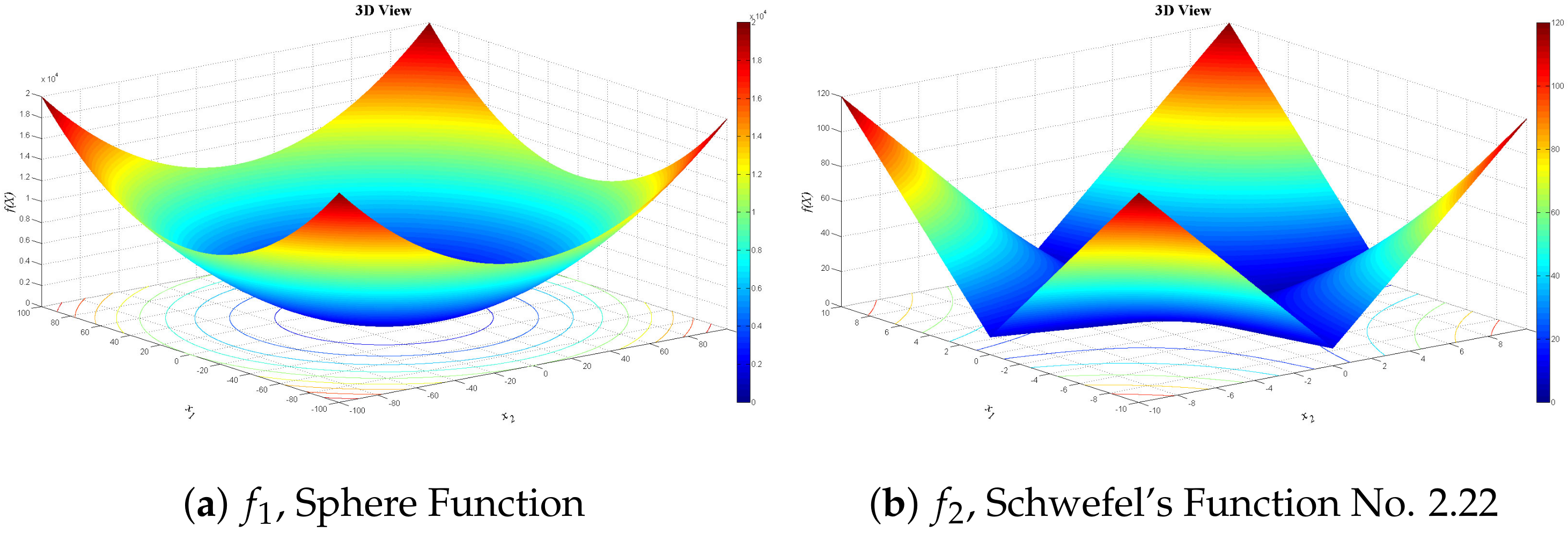
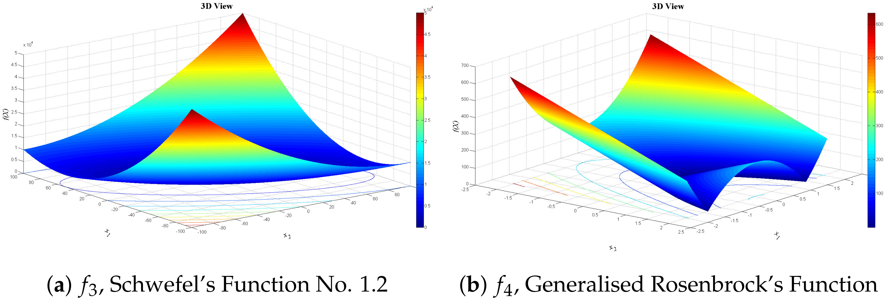
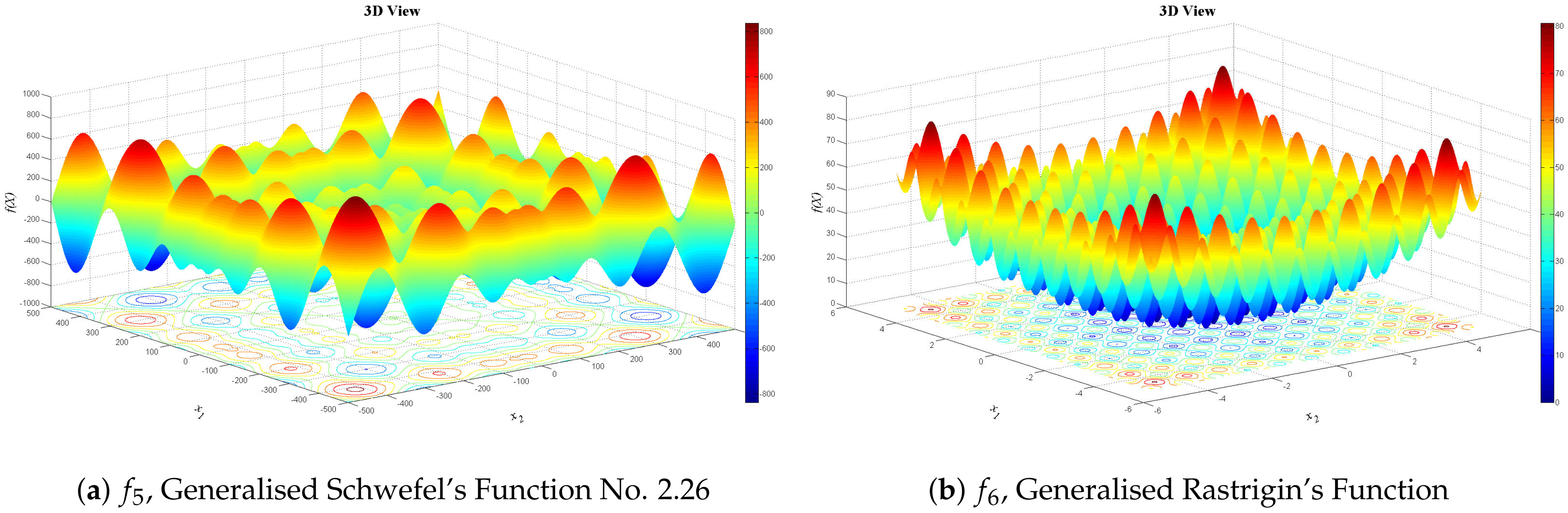
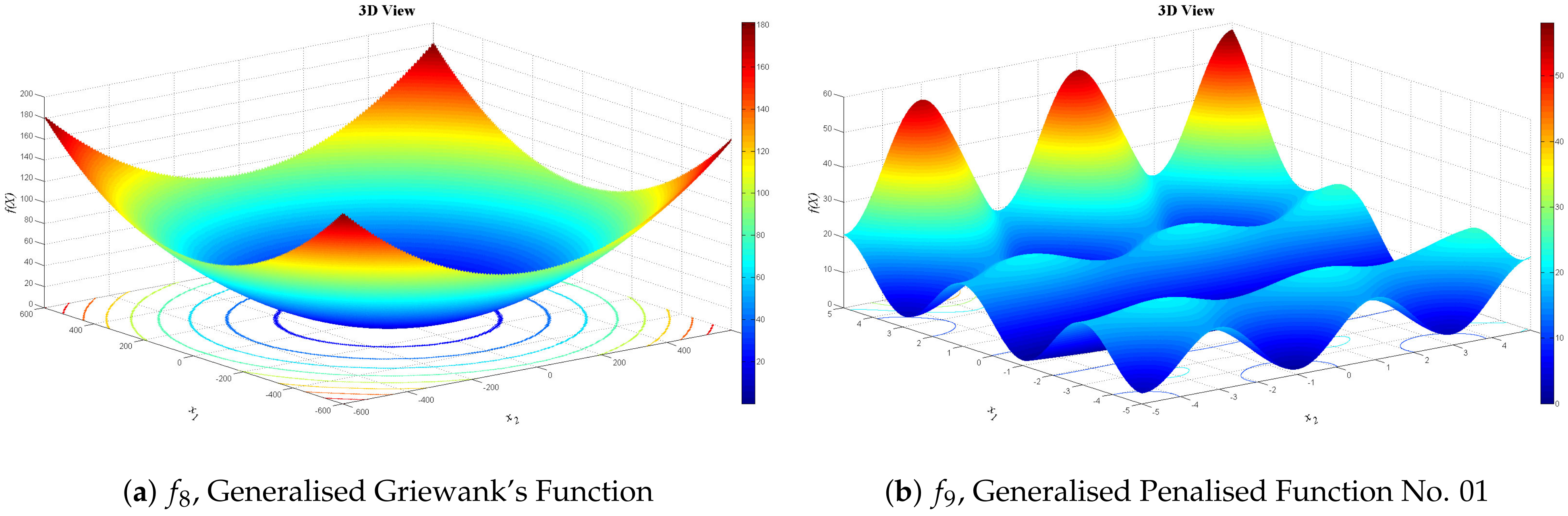
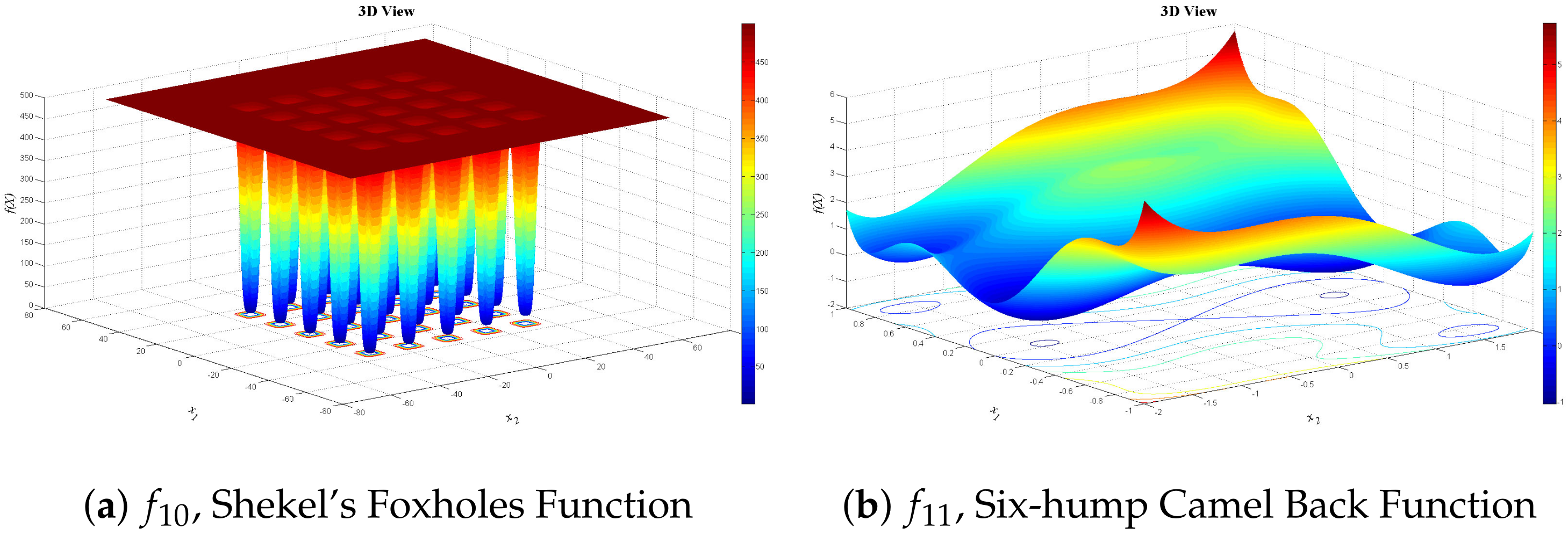
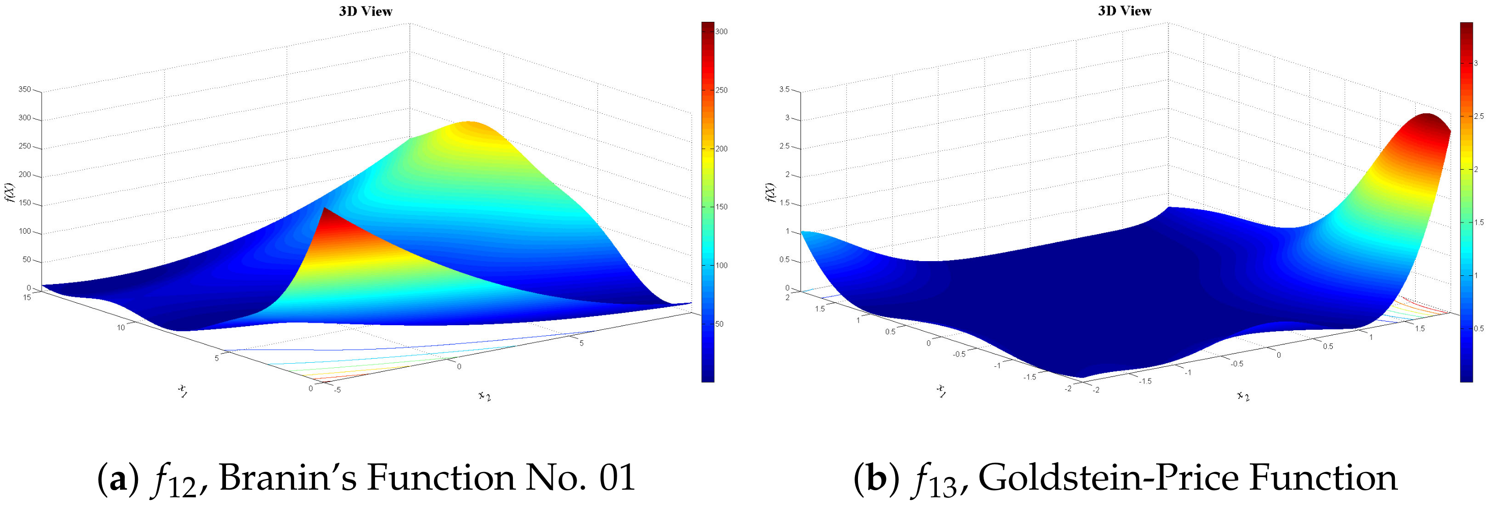
4.1. Benchmark Test Functions

In order to test the performance and demonstrate the efficiency of our proposed hybrid approach, we applied 15 well-known benchmark function,

Table 3. Optimum values reported for the benchmark functions in the literature, with their corresponding solutions and search subsets.

Function	Search Subsets	Opt	Sol
$f_1$(x)	${[-100,100]}^{30}$	0	${\left[0\right]}^{30}$
$f_2$(x)	${[-10,10]}^{30}$	0	${\left[0\right]}^{30}$
$f_3$(x)	${[-100,100]}^{30}$	0	${\left[0\right]}^{30}$
$f_4$(x)	${[-30,30]}^{30}$	0	${\left[1\right]}^{30}$
$f_5$(x)	${[-500,500]}^{30}$	−12,596.487	${\left[420.9687\right]}^{30}$
$f_6$(x)	${[-5.12,5.12]}^{30}$	0	${\left[0\right]}^{30}$
$f_7$(x)	${[-32,32]}^{30}$	0	${\left[0\right]}^{30}$
$f_8$(x)	${[-600,600]}^{30}$	0	${\left[0\right]}^{30}$
$f_9$(x)	${[-50,50]}^{30}$	0	${\left[1\right]}^{30}$
$f_{10}$(x)	${[-65.536,65.536]}^2$	1	${[-32]}^2$
$f_{11}$(x)	${[-5,5]}^2$	−1.0316285	(0.08983, −0.7126) and (−0.08983, 0.7126)
$f_{12}$(x)	$[-5,10]$ for $x_1$ and $[0,15]$ for $x_2$	0.397887	(−3.142, 12.275), (3.142, 2.275), and (9.425, 2.425)
$f_{13}$(x)	${[-2,2]}^2$	3	(0, −1)
$f_{14}$(x)	${[0,1]}^3$	−3.86	(0.114, 0.556, 0.852)
$f_{15}$(x)	${[0,1]}^6$	−3.32	(0.201, 0.150, 0.477, 0.275, 0.275, 0.377, 0.657)

. These function are divided into three main categories, such as unimodal [45] represented in Equations (11)–(14) and Figure 4 and Figure 5, multimodal [46] represented in Equations (15)–(19) and Figure 6 and Figure 7, and fixed-dimension multimodal [45,46], Equations (20)–(25) and Figure 8 and Figure 9. Regarding the features of these functions, $f_1$ to $f_9$ are high-dimensional problems. On the other hand, $f_{10}$ to $f_{15}$ comprehends low-dimensional problems. Additionally, all test functions reflect different degrees of complexity, $f_1$ to $f_4$ are convex, $f_7$, $f_{11}$, and $f_{13}$ are non-convex, $f_5$, $f_6$, and $f_8$ are non-linear functions. Regarding the justification behind the selection of this set of functions, $f_1$ to $f_4$ have only one global optimum and has no local optima, which makes this first group of functions highly appropriate to study the convergence rate and intensification ability of our proposed approach. Additionally, $f_5$ to $f_{15}$ concerns large search space and multiple local solutions besides the global optimum. Thus, they are useful evaluating how efficient the approach is avoiding local optima and the diversification abilities. Additionally, it is well-known that functions from the second group, $f_5$ to $f_9$, correspond to a group of very difficult problems to solve for optimisation algorithms, where there is an exponentially increase in number of dimensions [47]. Finally, all these functions are minimisation problems.

Unimodal functions:

Sphere Function

$$f_1\left(x\right)=f(x_1,x_2,...,x_n)=\sum _{i=1}^n{x}_i^2$$

(11)

Schwefel’s Function No. 2.22

$$f_2\left(x\right)=\sum _{i=1}^n|x_i|+\prod _{i=1}^n\left|x_i\right|$$

(12)

Schwefel’s Function No. 1.2

$$f_3\left(x\right)=\sum _{i=1}^n{\left(\sum _{j=1}^i{x}_j\right)}^2$$

(13)

Generalised Rosenbrock’s Function

$$f_4\left(x\right)=\sum _{i=1}^{n-1}\left[100{(x_i^2-x_{i+1})}^2+{(1-x_i)}^2\right]$$

(14)

Multimodal functions:

Generalised Schwefel’s Function No. 2.26

$$f_5\left(x\right)=-\sum _{i=1}^n{x}_{i}sin\left(\sqrt{|x_i|}\right)$$

(15)

Generalised Rastrigin’s Function

$$f_6\left(x\right)=10n+\sum _{i=1}^n(x_i^2-10cos\left(2\pi x_i\right))$$

(16)

Ackley’s Function

$$f_7\left(x\right)=-20exp(-0.2\sqrt{\frac{1}{n}{\sum }_{i=1}^n{x}_i^2})-exp(\frac{1}{n}\sum _{i=1}^{n}cos(2\pi x_i))+20+exp\left(1\right)$$

(17)

Generalised Griewank’s Function

$$f_8\left(x\right)=1+\sum _{i=1}^n\frac{x_i^2}{4000}-\prod _{i=1}^{n}cos(\frac{x_i}{\sqrt{i}})$$

(18)

Generalised Penalised Function

$$\begin{array}{c}\hfill f_9\left(x\right)=\frac{\pi }{n}\times \left\{10{sin}^2\left(\pi y_1\right)+\sum _{i=1}^{n-1}{\left(y_i-1\right)}^2\left[1+10{sin}^2\left(\pi y_{i+1}\right)\right]+{\left(y_n-1\right)}^2\right\}\\ \hfill +\sum _{i=1}^{n}u\left(x_i,10,100,4\right)\end{array}$$

(19)

where $u(x_i,a,k,m)$ is equal to

• $k{(x_i-a)}^m$ if $x_i>a$
• 0 if $-a\le x_i\le a$
• $k{(-x_i-a)}^m$ if $x_i<-a$

and

• $y_i=1+\frac{1}{4}(x_i+1)$

Multimodal functions with fixed dimensions:

Shekel’s Foxholes Function

$$f_{10}\left(x\right)={\left[\frac{1}{500}+\sum _{j=1}^{25}\frac{1}{j+{\sum }_{i=1}^2{\left(x_i-a_{i,j}\right)}^6}\right]}^{-1}$$

(20)

where:

$a_{i,j}=\left[\begin{array}{cccccccccc}-32& -16& 0& 16& 32& -32& ...& 0& 16& 32\\ -32& -32& -32& -32& -32& -16& ...& 32& 32& 32\end{array}\right]$

Six-hump Camel Back Function

$$f_{11}\left(x\right)=4x_1^2-2.1x_1^4+\frac{1}{3}{x}_1^6+x_1{x}_2-4x_2^2+4x_2^4$$

(21)

Branin’s Function

$$f_{12}\left(x\right)={\left(x_2-\frac{5.1x_1^2}{4{\pi }^2}+\frac{5x_1}{\pi }-6\right)}^2+10\left(1-\frac{1}{8\pi }\right)cos\left(x_1\right)+10$$

(22)

Goldstein-Price Function

$$\begin{array}{c}\hfill f_{13}\left(x\right)=\left[1+{\left(x_1+x_2+1\right)}^2\left(19-14x_1+3x_1^2-14x_2+6x_1{x}_2+3x_2^2\right)\right]\\ \hfill \left[30+{\left(2x_1-3x_2\right)}^2\left(18-32x_1+12x_1^2+48x_2-36x_1{x}_2+27x_2^2\right)\right]\end{array}$$

(23)

Hartman’s Function No.1

$$f_{14}\left(x\right)=-\sum _{i=1}^4{c}_i{e}^{{\displaystyle \left[-\sum _{j=1}^3{a}_{i,j}{\left(x_j-p_{i,j}\right)}^2\right]}}$$

(24)

where the values of a, c, and p are tabulated in

Table 4. Values of $a_{ij}$, $c_i$, and $p_{ij}$ for function $f_{1}4$(x); n = 3 and j = 1, 2, 3.

i	${\mathit{a}}_{\mathit{ij}}$			${\mathit{c}}_{\mathit{i}}$	${\mathit{p}}_{\mathit{ij}}$
1	3	10	30	1	0.3689	0.1170	0.2673
2	0.1	10	35	1.2	0.4699	0.4387	0.7470
3	3	10	30	3	0.1091	0.8732	0.5547
4	0.1	10	30	3.2	0.03815	0.5743	0.8828

Hartman’s Function No.2

$$f_{15}\left(x\right)=-\sum _{i=1}^4{c}_i{e}^{{\displaystyle \left[-\sum _{j=1}^6{a}_{i,j}{\left(x_j-p_{i,j}\right)}^2\right]}}$$

(25)

where the values of a, c and p are tabulated in

Table 5. Values of $a_{ij}$, $c_i$, and $p_{ij}$ for function $f_{1}5$(x); n = 6 and j = 1, 2, ..., 6.

i	${\mathit{a}}_{\mathit{ij}}$						${\mathit{c}}_{\mathit{i}}$	${\mathit{p}}_{\mathit{ij}}$
1	10	3	17	3.5	1.7	8	1	0.131	0.169	0.556	0.012	0.828	0.588
2	0.05	10	17	0.1	8	14	1.2	0.232	0.413	0.830	0.373	0.100	0.999
3	3	3.5	1.7	10	17	8	3	0.234	0.141	0.352	0.288	0.304	0.665
4	17	8	0.05	10	0.1	14	3.2	0.404	0.882	0.873	0.574	0.109	0.038

.

4.2. Algorithms Used for Comparison and Experimental Setup

In order to compare the results obtained, we designed this step in three phases. First phase, we compare against state-of-the-art optimisation methods reported in [18,19,48], such as particle swarm optimisation (PSO) [15], gravitational search algorithm (GSA) [16], differential evolution (DE) [17], whale optimisation algorithm (WOA) [18], vapour–liquid equilibrium (VLE) [19], and an hybrid between Nelder–Mead algorithm and dragonfly algorithm (INMDA) [20]. In the second phase we compare against SPO [21], which is a heuristic that combines classical and modern statistical techniques to improve the performance of search algorithms. Finally, we take a closer look at the performance achieved by the traditional SHO, a neural network (NN) [22], and a sine cosine algorithm (SCA) [23] approach solving the benchmark functions in comparison with our proposed approach. Regarding the implementation of traditional SHO, the number of search agents was set to 30, control parameter h with values in range of [5, 0], the constant M in the range of [0.5, 1], and the value for number of generations was 10,000. Regarding the neural network, the design was defined as follows: For each benchmark function, a total of one million randomly generated solutions were created. On the other hand, we designed a multi-layer perceptron. The main components comprehend an input node, 7 hidden layers of 50 nodes, and an output equal to the number of dimensions for each function. The training was carried out employing the gradient descent method [49] over 1000 iterations for each randomly generated solution. The main objective behind the NN proposed is the prediction of better function values on run-time. The implementation was performed in python 3.7 and run in an environment windows 10 with 64 bits on Core i-5 processor with 2.40 GHz and 8 GB memory. Finally, regarding the experimentation phase, for each benchmark function the algorithm utilises 30 independent runs.

4.3. Performance Comparison

In this subsection, we illustrate and demonstrate the performance of our proposed $L{B}^2$ tackling the benchmark functions described in the Section 4.1.

4.3.1. First Experimentation Phase

First, all results obtained by SHO and $L{B}^2$ were rounded to four decimals. The results published for PSO, GSA, DE, WOA, and VLE, were rounded in

Table 6. Results comparison in unimodal benchmark functions.

F	SHO		${\mathit{LB}}^2$		WOA		DE		GSA		PSO		VLE		INMDA
	Avg	StdDev	Avg	StdDev	Avg	StdDev	Avg	StdDev	Avg	StdDev	Avg	StdDev	Avg	StdDev	Avg	StdDev
$f_1$	0.0006	0.0005	0.0000	0.0000	0.0000	0.0000	$8.2000\times {10}^{-14}$	$5.9000\times {10}^{-14}$	$2.5300\times {10}^{-16}$	0.0000	$1.3600\times {10}^{-4}$	$2.0200\times {10}^{-4}$	$4.4989\times {10}^{-7}$	$1.413\times {10}^{-6}$	0.0000	0.0000
$f_2$	0.0000	0.0000	0.0000	0.0000	0.0000	0.0000	$1.5000\times {10}^{-9}$	$9.9000\times {10}^{-10}$	$5.5655\times {10}^{-2}$	0.1941	$4.2144\times {10}^{-2}$	$4.5421\times {10}^{-2}$	$3.0840\times {10}^{-6}$	$6.0498\times {10}^{-6}$	0.0000	0.0000
$f_3$	0.0007	0.0005	0.0000	0.0000	$5.3900\times {10}^{-7}$	$2.9300\times {10}^{-6}$	$6.8000\times {10}^{-11}$	$7.4000\times {10}^{-11}$	$8.9353\times {10}^2$	$3.1896\times {10}^2$	70.126	22.119	5.2020	0.7986	0.0000	0.0000
$f_4$	2.7511	0.0502	$6.7549\times {10}^{-7}$	$5.4204\times {10}^{-7}$	27.866	0.7636	0.0000	0.0000	67.543	62.225	96.718	60.116	79.199	37.400	0.0000	0.0000

,

Table 7. Results comparison in multimodal benchmark functions.

F	SHO		${\mathit{LB}}^2$		WOA		DE		GSA		PSO		VLE		INMDA
	Avg	StdDev	Avg	StdDev	Avg	StdDev	Avg	StdDev	Avg	StdDev	Avg	StdDev	Avg	StdDev	Avg	StdDev
$f_5$	$-1.0867\times {10}^4$	0.5059	$-\mathbf{1}.\mathbf{2569}\times {\mathbf{10}}^{\mathbf{4}}$	0.0014	$-5.0808\times {10}^3$	$6.9580\times {10}^2$	$-1.1080\times {10}^4$	$5.7470\times {10}^2$	$-2.8211\times {10}^3$	$4.9304\times {10}^2$	$-4.8413\times {10}^3$	$1.1528\times {10}^3$	$-1.2566\times {10}^4$	68.705	−2245.1500	2.8400
$f_6$	0.0000	0.0000	0.0000	0.0000	0.0000	0.0000	69.200	38.800	25.968	7.4701	46.704	11.629	34.5830	17.8860	0.0000	0.0000
$f_7$	$4.4408\times {10}^{-16}$	0.0000	$4.4409\times {10}^{-16}$	0.0000	7.4043	9.8976	$9.7000\times {10}^{-8}$	$4.2000\times {10}^{-8}$	$6.2087\times {10}^{-2}$	0.23628	0.27602	0.50901	3.1704	3.9211	0.0000	$1.6200\times {10}^{-16}$
$f_8$	0.0000	0.0000	0.0000	0.0000	$2.8900\times {10}^{-4}$	$1.5860\times {10}^{-3}$	0.0000	0.0000	27.702	5.0403	$9.2150\times {10}^{-3}$	$7.7240\times {10}^{-3}$	0.5074	0.5041	0.0000	0.0000
$f_9$	1.906	0.0865	1.8286	$1.5985\times {10}^{-9}$	0.3397	0.2149	$7.9000\times {10}^{-15}$	$8.0000\times {10}^{-15}$	1.7996	0.95114	$6.9170\times {10}^{-3}$	$2.6301\times {10}^{-2}$	0.2369	0.2877	0.0000	0.0000

and

Table 8. Results comparison in multimodal benchmark functions with fixed-dimension.

F	SHO		${\mathit{LB}}^2$		WOA		DE		GSA		PSO		VLE		INMDA
	Avg	StdDev	Avg	StdDev	Avg	StdDev	Avg	StdDev	Avg	StdDev	Avg	StdDev	Avg	StdDev	Avg	StdDev
$f_{10}$	$2.1326\times {10}^{-8}$	$5.0161\times {10}^{-10}$	1.0000	0.0000	2.1120	2.4986	0.99800	$3.3000\times {10}^{-16}$	5.8598	3.8313	3.6272	2.5608	0.99800	$2.5294\times {10}^{-7}$	N/A	N/A
$f_{11}$	0.0000	0.0000	0.0000	0.0000	−1.0316	$4.2000\times {10}^{-7}$	−1.0316	$3.1000\times {10}^{-13}$	−1.0316	$4.8800\times {10}^{-16}$	−1.0316	$6.2500\times {10}^{-16}$	−1.0315	$1.8408\times {10}^{-4}$	N/A	N/A
$f_{12}$	0.8718	0.0502	1.5436	0.4223	0.39791	$2.7000\times {10}^{-5}$	0.39789	$9.9000\times {10}^{-9}$	0.39789	0.0000	0.39789	0.0000	0.39815	$4.5697\times {10}^{-4}$	N/A	N/A
$f_{13}$	36.0716	4.1607	32.6845	$1.4854\times {10}^{-8}$	3.0000	$4.2200\times {10}^{-15}$	3.0000	$2.0000\times {10}^{-15}$	3.0000	$4.1700\times {10}^{-15}$	3.0000	$1.3300\times {10}^{-15}$	3.0097	$1.6256\times {10}^{-2}$	N/A	N/A
$f_{14}$	−2.1211	0.1284	−2.0081	$5.0800\times {10}^{-10}$	−3.8562	$2.7060\times {10}^{-3}$	N/A	N/A	−3.8628	$2.2900\times {10}^{-15}$	−3.8628	$2.5800\times {10}^{-15}$	−3.8628	$6.6880\times {10}^{-5}$	N/A	N/A
$f_{15}$	−0.8515	0.3541	−1.5870	0.5016	−2.9811	0.37665	N/A	N/A	−3.3178	$2.3081\times {10}^{-2}$	−3.2663	$6.0516\times {10}^{-2}$	−3.3179	$2.1311\times {10}^{-2}$	N/A	N/A

to four decimals, using scientific notation, only for presentation purposes. However, all computations were carried out using the reported decimals by their respective authors. Regarding the performance on unimodal functions, Table 6 illustrates the results and comparison in $f_1$ to $f_4$, the average (Avg) and standard deviation (StdDev) are presented and compared, and we highlight in bold the best values reached. Additionally, it is well-known that unimodal functions can help us to measure the exploitation capabilities of our proposed approach. In this regard, it is surprising how good $L{B}^2$ performed. It was the second most efficient algorithm tackling this set of benchmark function just behind INMDA. Additionally, the small values reached corresponding to the StdDev shows that it is a very solid algorithm. Concerning the multimodal functions and multimodal functions with fixed dimensions, both sets can help us to evaluate the potential of our algorithm in carrying out the exploration. Table 7 and Table 8 illustrates the results and comparison on functions $f_5$ to $f_9$ and $f_{10}$ to $f_{15}$ correspondingly, the average (Avg) and standard deviation (StdDev) are presented, and we highlight in bold the best values reached. Surprisingly, the $L{B}^2$ attained really good results and small Avg and StdDev values once again, proving to be a competitive approach able to tackle continuous problems. Moreover, having a relatively good performance in these three previous set of benchmark test functions, we can conclude that this first attempt corresponding to the $L{B}^2$ has the potential to be a competitive approach.

4.3.2. Second Experimentation Phase

In this subsection, we compare against SPO, which has proved to be a good and competitive option in the field of parameter tuning. In this work, we compare the results obtained by our $L{B}^2$ against the works reported and implemented in [21]. They implemented a PSO and a PSO + SPO approach, they solve 4 benchmark test functions.

Table 9. Comparison results of SPO against $L{B}^2$ proposed.

Problem	PSO	PSO + SPO	${\mathit{LB}}^2$
Sphere	$2.82\times {10}^{-9}$	$1.66\times {10}^{-21}$	0
Rosenbrock	148.84	4.20	0
Rastrigin	10.43	0.98	0
Griewangk	0.12	0.07	0

illustrates the best values reached, where the first column, named problem, represent the 4 functions solved by the approach reported (2 unimodal and 2 multimodal). Column 2, 3, and 4, represent the best values achieved by PSO and PSO + SPO (both implemented by the authors), and our proposed $L{B}^2$. It is clear the superiority of our approach reaching all 4 optimum values. However, in future work, in order to improve the hybrid methodology proposed in this work, we have as an objective the implementation and comparison of SPO and F-Race approaches in order to bring a more detailed and larger competition between multiple optimisation and tuning tools.

4.3.3. Third Experimentation Phase

In this subsection, we present a comparison of $L{B}^2$ against a traditional SHO and a neural network approach, both implementation made by us.

Table 10. Results comparison of SHO vs. $L{B}^2$.

F	Opt	SHO					${\mathit{LB}}^2$
		Best	Worst	Avg	StdDev	Avg Time(s)	Best	Worst	Avg	StdDev	Avg Time(s)
$f_1$	0	0	0.0021	0.0006	0.0005	51.6432	0	0	0	0	50.2377
$f_2$	0	0	0	0	0	78.9275	0	0	0	0	80.7524
$f_3$	0	0	0.0009	0.0007	0.0005	95.5684	0	0	0	0	96.3627
$f_4$	0	2.7091	2.9351	2.7511	0.0502	75.8810	$1.59197\times {10}^{-7}$	$1.2262\times {10}^{-6}$	$6.7549\times {10}^{-7}$	$5.4204\times {10}^{-7}$	71.0024
$f_5$	−12,569.487	$-1.1318\times {10}^4$	$-0.9653\times {10}^4$	$-1.0867\times {10}^4$	0.5059	121.3511	$-1.2570\times {10}^4$	$-1.2567\times {10}^4$	$-1.2569\times {10}^4$	0.0014	110.3354
$f_6$	0	0	0	0	0	172.9312	0	0	0	0	60.6482
$f_7$	0	$4.4408\times {10}^{-16}$	$4.4408\times {10}^{-16}$	$4.4408\times {10}^{-16}$	0	256.8700	$4.4408\times {10}^{-16}$	$4.4409\times {10}^{-16}$	$4.4409\times {10}^{-16}$	0	24.9122
$f_8$	0	0	0	0	0	198.8546	0	0	0	0	21.7758
$f_9$	0	1.8290	2.5642	1.906	0.0865	256.8707	1.8285	1.8286	1.8286	$1.5985\times {10}^{-9}$	24.9172
$f_{10}$	1	$2.1745\times {10}^{-8}$	$2.0745\times {10}^{-8}$	$2.1326\times {10}^{-8}$	$5.0161\times {10}^{-10}$	130.3552	1	1	1	0	17.5661
$f_{11}$	−1.0316	0	0	0	0	29.1582	0	0	0	0	7.5244
$f_{12}$	0.3979	0.8298	0.9523	0.8718	0.0502	22.5778	1.1905	2.0325	1.5436	0.4223	4.5528
$f_{13}$	3	32.6845	44.4562	36.0716	4.1607	35.7789	32.6845	32.6845	32.6845	$1.4854\times {10}^{-8}$	3.6846
$f_{14}$	−3.86	−2.4301	−2.0081	−2.211	0.1284	53.2235	−2.0081	−2.0080	−2.0081	$5.0800\times {10}^{-10}$	7.1120
$f_{15}$	−3.32	−1.1676	−0.4676	−0.8515	0.3541	80.4755	−2.1676	−2.1676	−2.1676	0	8.1145

,

Table 11. Results comparison of NN vs. $L{B}^2$.

F	Opt	NN					${\mathit{LB}}^2$
		Best	Worst	Avg	StdDev	Avg Time(s)	Best	Worst	Avg	StdDev	Avg Time(s)
$f_1$	0	0.0639	0.2223	0.1068	0.0435	347.4073	0	0	0	0	50.2377
$f_2$	0	1.2426	5.8827	4.4004	0.8284	375.2112	0	0	0	0	80.7524
$f_3$	0	0.0001	0.0379	0.0103	0.0108	377.0420	0	0	0	0	96.3627
$f_4$	0	211.4253	3037.6363	1376.6472	1041.5627	375.6543	$1.59197\times {10}^{-7}$	$1.2262\times {10}^{-6}$	$6.7549\times {10}^{-7}$	$5.4204\times {10}^{-7}$	71.0024
$f_5$	−12,569.487	$-1.2557\times {10}^4$	$-1.7363\times {10}^4$	$-1.2057\times {10}^4$	2056.9973	357.8577	$-1.2570\times {10}^4$	$-1.2567\times {10}^4$	$-1.2569\times {10}^4$	0.0014	110.3354
$f_6$	0	1.8672	7.8028	4.2664	1.5939	357.7703	0	0	0	0	60.6482
$f_7$	0	0.2687	0.5169	0.3905	0.0689	350.7136	$4.4408\times {10}^{-16}$	$4.4409\times {10}^{-16}$	$4.4409\times {10}^{-16}$	0	24.9122
$f_8$	0	0.0416	1.1238	0.8017	0.1986	354.9282	0	0	0	0	21.7758
$f_9$	0	29,752,063.66	29,800,464.52	29,792,019.73	9855.6445	357.1411	1.8285	1.8286	1.8286	$1.5985\times {10}^{-9}$	24.9172
$f_{10}$	1	0.0160	495.8931	214.7364	200.8041	343.9354	1	1	1	0	17.5661
$f_{11}$	−1.0316	−0.0079	0.0103	0.0005	0.0041	344.4559	0	0	0	0	7.5244
$f_{12}$	0.3979	10.0004	16.3393	12.2766	1.3941	369.1712	1.1905	2.0325	1.5436	0.4223	4.5528
$f_{13}$	3	3.0227	5.4062	5.3044	1.5586	369.8705	32.6845	32.6845	32.6845	$1.4854\times {10}^{-8}$	3.6846
$f_{14}$	−3.86	−3.8417	−3.5163	−3.7177	0.0913	376.6538	−2.0081	−2.0080	−2.0081	$5.0800\times {10}^{-10}$	7.1120
$f_{15}$	−3.32	−1.4809	−0.7560	−1.0409	0.2019	342.6122	−2.1676	−2.1676	−2.1676	0	8.1145

and

Table 12. Results comparison of SCA vs. $L{B}^2$.

F	Opt	SCA					${\mathit{LB}}^2$
		Best	Worst	Avg	StdDev	Avg Time(s)	Best	Worst	Avg	StdDev	Avg time(s)
$f_1$	0	0	0	0	0	10.4656	0	0	0	0	50.2377
$f_2$	0	0	0	0	0	17.3875	0	0	0	0	80.7524
$f_3$	0	0	0	0	0	74.3906	0	0	0	0	96.3627
$f_4$	0	$1.33\times {10}^{-10}$	29	17.4000	14.9755	13.4296	$1.59197\times {10}^{-7}$	$1.2262\times {10}^{-6}$	$6.7549\times {10}^{-7}$	$5.4204\times {10}^{-7}$	71.0024
$f_5$	−12,569.487	$2.51\times {10}^{-7}$	0.0696	0.0181	0.0251	9.5828	$-1.2570\times {10}^4$	$-1.2567\times {10}^4$	$-1.2569\times {10}^4$	0.0014	110.3354
$f_6$	0	0	0	0	0	11.2296	0	0	0	0	60.6482
$f_7$	0	$4.44\times {10}^{-16}$	$4.44\times {10}^{-16}$	$4.44\times {10}^{-16}$	0	15.1140	$4.4408\times {10}^{-16}$	$4.4409\times {10}^{-16}$	$4.4409\times {10}^{-16}$	0	24.9122
$f_8$	0	0	0	0	0	13.3500	0	0	0	0	21.7758
$f_9$	0	1.8285	1.8416	1.8304	0.0042	78.2046	1.8285	1.8286	1.8286	$1.5985\times {10}^{-9}$	24.9172
$f_{10}$	1	0.0003	4.9301	1.0010	2.0705	28.9609	1	1	1	0	17.5661
$f_{11}$	−1.0316	1.0316	1.0316	1.0316	$2.3406\times {10}^{-16}$	2.7093	0	0	0	0	7.5244
$f_{12}$	0.3979	0.1555	3.9503	1.1009	1.3759	2.9765	1.1905	2.0325	1.5436	0.4223	4.5528
$f_{13}$	3	29.6845	30.0547	29.7444	0.1229	4.1765	32.6845	32.6845	32.6845	$1.4854\times {10}^{-8}$	3.6846
$f_{14}$	−3.86	1.8519	1.8519	1.8519	0	7.0265	−2.0081	−2.0080	−2.0081	$5.0800\times {10}^{-10}$	7.1120
$f_{15}$	−3.32	2.1523	2.1524	2.1524	0	9.5578	−2.1676	−2.1676	−2.1676	0	8.1145

illustrates a summary of the values achieved in the experimentation phase. Column F corresponds to the test function solved, and Opt depicts the global optimum for the given function. Column best, worst, and Avg are the given values for best value reached, worst value reached, the mean value, and the Avg time achieved in 30 executions.

Regarding Table 10, $L{B}^2$ achieved 7 optimum values in $f_1$–$f_3$, $f_5$, $f_6$, $f_8$, and $f_{10}$, in comparison of SHO which achieved 5 optimum values in $f_1$–$f_3$, $f_6$, $f_8$. Additionally, regarding non-optimum values reached, our proposed approach is superior in 5 values in functions $f_4$, $f_5$, $f_9$,$f_{13}$, and $f_{15}$. However, the same goes for SHO in functions $f_{11}$, $f_{12}$, and $f_{14}$. Regarding Table 9, $L{B}^2$ achieve better values than the NN approach implemented. However, in functions $f_{13}$ and $f_{14}$ the performance of our proposed approach falls behind considerably. Regarding Table 12, small differences can be observed, $L{B}^2$ reached 1 more optimum value. However, the biggest difference concerns the robustness in the overall performance illustrated on columns Avg and StdDev. This can be observed in functions $f_4$, $f_5$, and $f_{10}$.

Regarding the average time achieved in the three illustrated tables, significant difference can be observed between NN, SCA, and $L{B}^2$. In the hardest test function, multimodal, and multimodal with fixed-dimension, NN falls significantly behind against SCA and $L{B}^2$ in solving time, which is the strong point on these types of algorithms. Additionally, we highlight the drawback behind a NN approach, the costly process of training and tuning of the model. Nevertheless, the objective behind this test, presented in Table 11, concerns the future incorporation of new learning methods to $L{B}^2$.

Regarding the room for improvements observed in the performance, values achieved in column StdDev for $f_5$, $f_{11}$, $f_{14}$, and $f_{15}$ can be interpreted as the approach being trapped in local optima. The discussion follows two possible issues: the value employed as $\beta$ and the scheme values for the diversification process. Firstly, the proposed value for threshold $\beta$ is static through the search, the consequence can be interpreted as the approach expecting a more balanced and timely feedback from the learning model. Thus, when a local optima is detected, a proper answer can be delivered and carried out on run-time. Nevertheless, the incorporation of a learning-based component managing a dynamic $\beta$ value on run-time will be proposed in order to tackle this issue. On the other hand, regarding the scheme values for diversification, the employment of static values through the search can be a critical issue. The amount and frequency on which diversification is carried out will be our next focus as a balanced exploration in the search space needs to be performed.

In order to further analyse and demonstrate the improvement in the performance of the hybridisation in optimisation tools, a statistical analysis is carried out. To this end we compare convergence and we analyse the 30 executions performed for each function through the Kolmogorov Smirnov Lilliefors (Lilliefors 1967) [50] and Wilcoxon’s signed rank (Mann and Whitney 1947) [51] statistical tests. Additionally, in order to carry the statistical analysis of this phase, we make use of the RStudio software to conduct both tests.

The process is as follows, samples were tested for normality using Kolmogorov Smirnov Lilliefors test, having failed it (p-values > 0.05). Therefore, the non-parametric Mann-Whitney test subsequently used to compare the quality of SHO and $L{B}^2$ results. We need to take in consideration the next two hypothesis:

$$H_0:{\mu }_{SHO}={\mu }_{L{B}^2}$$

$$H_1:{\mu }_{L{B}^2}\ne {\mu }_{SHO}$$

where ${\mu }_{SHO}$ and ${\mu }_{L{B}^2}$ are the arithmetic median of fitness values achieved corresponding to SHO and our proposed $L{B}^2$. Again, at this next step we take into consideration that the significance level is also established to 0.05, thus, smaller values that 0.05 defines that $H_0$ cannot be assumed. In this regard,

Table 13. Exact p values obtained on the benchmark test functions.

F		SHO	${\mathit{LB}}^2$
$f_1$	SHO	-	>0.05
	$L{B}^2$	>0.05	-
$f_2$	SHO	-	>0.05
	$L{B}^2$	>0.05	-
$f_3$	SHO	-	>0.05
	$L{B}^2$	>0.05	-
$f_4$	SHO	-	$\mathbf{2}.\mathbf{35}\times {\mathbf{10}}^{-\mathbf{18}}$
	$L{B}^2$	>0.05	-
$f_5$	SHO	-	$\mathbf{6}.\mathbf{611}\times {\mathbf{10}}^{-\mathbf{7}}$
	$L{B}^2$	>0.05	-
$f_6$	SHO	-	>0.05
	$L{B}^2$	>0.05	-
$f_7$	SHO	-	>0.05
	$L{B}^2$	>0.05	-
$f_8$	SHO	-	>0.05
	$L{B}^2$	>0.05	-
$f_9$	SHO	-	$\mathbf{7}.\mathbf{01}\times {\mathbf{10}}^{-\mathbf{7}}$
	$L{B}^2$	>0.05	-
$f_{10}$	SHO	-	$\mathbf{1}.\mathbf{1}\times {\mathbf{10}}^{-\mathbf{7}}$
	$L{B}^2$	>0.05	-
$f_{11}$	SHO	-	0.02067
	$L{B}^2$	>0.05	-
$f_{12}$	SHO	-	>0.05
	$L{B}^2$	0.04	-
$f_{13}$	SHO	-	>0.05
	$L{B}^2$	>0.05	-
$f_{14}$	SHO	-	$\mathbf{1}.\mathbf{395}\times {\mathbf{10}}^{-\mathbf{6}}$
	$L{B}^2$	>0.05	-
$f_{15}$	SHO	-	$\mathbf{1}.\mathbf{863}\times {\mathbf{10}}^{-\mathbf{9}}$
	$L{B}^2$	>0.05	-

illustrate the comparison between the two implementations, we highlight in bold the values where there is a statistically significant winner.

5. Conclusions and Future Work

In this paper, a novel learning-based framework was proposed. Well-known methods and techniques are employed to design a competitive hybrid approach capable to tackle on optimisation problems. The proposed framework performs under a population-based strategy, multiple agents explore, learn, and evolve in the search space. In this regard, two main components were employed: a population-based algorithm, named spotted hyena optimiser, and a learning model which is based in a statistical modelling method.

Regarding the results achieved solving the benchmark functions, $L{B}^2$ demonstrated to be a competitive method and a promising alternative to tackle optimisation problems. However, some issues remains and improvements can be proposed. Firstly, $L{B}^2$ needs to be tested tackling benchmark functions with higher difficulty. In this regard, we are considering more complex functions with higher dimensionality, such as CEC 2021’s composite functions. Additionally, the incorporation of hard optimisation problems, such as set covering problem (SCP), manufacturing cell design problem (MCDP) are being considered as future testing objectives. On another hand, results illustrated in the third experimentation phase can be interpreted as $L{B}^2$ being trapped in local optima for certain functions. Nevertheless, improvements can be carried out in order to tackle this issue. In this regard, new learning-based components will be proposed. The main objective is to dynamically adjust parameters, such as threshold $\beta$ and the scheme for diversification and intensification. The idea is to keep the balance in the feedback of dynamic data and knowledge generated between the population and the learning model on run-time. Finally, new learning methods will be implemented, the objective concerns the viability, certainty, and confidence in the generated knowledge. Thus, a more complex component will be designed in order to measure the profit behind the knowledge for a better decision making through the search.

References

1. Talbi, E.G. Combining metaheuristics with mathematical programming, constraint programming and machine learning. Ann. Oper. Res. 2016, 240, 171–215. [Google Scholar] [CrossRef]
2. Gendreau, M.; Potvin, J.Y. Handbook of Metaheuristics, 2nd ed.; Springer: Berlin/Heidelberg, Germany, 2010. [Google Scholar]
3. Hussain, K.; Salleh, M.N.M.; Cheng, S.; Shi, Y. On the exploration and exploitation in popular swarm-based metaheuristic algorithms. Neural Comput. Appl. 2019, 31, 7665–7683. [Google Scholar] [CrossRef]
4. Chu, X.; Wu, T.; Weir, J.D.; Shi, Y.; Niu, B.; Li, L. Learning–interaction–diversification framework for swarm intelligence optimizers: A unified perspective. Neural Comput. Appl. 2020, 32, 1789–1809. [Google Scholar] [CrossRef]
5. Boussaïd, I.; Lepagnot, J.; Siarry, P. A survey on optimization metaheuristics. Inf. Sci. 2013, 237, 82–117. [Google Scholar] [CrossRef]
6. Tapia, D.; Crawford, B.; Soto, R.; Cisternas-Caneo, F.; Lemus-Romani, J.; Castillo, M.; García, J.; Palma, W.; Paredes, F.; Misra, S. A Q-Learning Hyperheuristic Binarization Framework to Balance Exploration and Exploitation. In International Conference on Applied Informatics; Springer: Cham, Switzerland, 2020; pp. 14–28. [Google Scholar]
7. Parsons, S. Introduction to Machine Learning by Ethem Alpaydin. In The Knowledge Engineering Review; MIT Press: Cambridge, MA, USA, 2005; Volume 20, pp. 432–433. [Google Scholar]
8. Song, H.; Triguero, I.; Özcan, E. A review on the self and dual interactions between machine learning and optimisation. Prog. Artif. Intell. 2019, 8, 143–165. [Google Scholar] [CrossRef] [Green Version]
9. Barber, D. Bayesian Reasoning and Machine Learning; Cambridge University Press: New York, NY, USA, 2012. [Google Scholar]
10. Lantz, B. Machine Learning with R; Packt Publishing: Birmingham, UK, 2013. [Google Scholar]
11. Dietterich, T. Machine Learning. ACM Comput. Surv. 1996, 28, 3. [Google Scholar] [CrossRef]
12. Dhiman, G.; Kumar, V. Spotted hyena optimizer: A novel bio-inspired based metaheuristic technique for engineering applications. Adv. Eng. Softw. 2017, 114, 48–70. [Google Scholar] [CrossRef]
13. Soto, R.; Crawford, B.; Vega, E.; Gómez, A.; Gómez-Pulido, J.A. Solving the Set Covering Problem Using Spotted Hyena Optimizer and Autonomous Search. Advances and Trends in Artificial Intelligence. From Theory to Practice. In IEA/AIE 2019; Springer: Cham, Swizterland, 2019; Volume 11606. [Google Scholar]
14. Luo, Q.; Li, J.; Zhou, Y.; Liao, L. Using spotted hyena optimizer for training feedforward neural networks. Cogn. Syst. Res. 2021, 65, 1–16. [Google Scholar] [CrossRef]
15. Kennedy, J.; Eberhart, R. Particle swarm optimization. In Proceedings of the IEEE International Conference on Neural Networks, Perth, Australia, 27 November–1 December 1995; pp. 1942–1948. [Google Scholar]
16. Rashedi, E.; Nezamabadi-Pour, H.; Saryazdi, S. GSA: A Gravitational Search Algorithm. Inf. Sci. 2009, 179, 2232–2248. [Google Scholar] [CrossRef]
17. Storn, R.; Price, K. Differential Evolution—A Simple and Efficient Heuristic for global Optimization over Continuous Spaces. J. Glob. Optim. 1997, 11, 341–359. [Google Scholar] [CrossRef]
18. Mirjalili, S.; Lewis, A. The Whale Optimization Algorithm. Adv. Eng. Softw. 2016, 95, 51–67. [Google Scholar] [CrossRef]
19. Cortés-Toro, E.M.; Crawford, B.; Gómez-Pulido, J.A.; Soto, R.; Lanza-Gutiérrez, J.M. A New Metaheuristic Inspired by the Vapour-Liquid Equilibrium for Continuous Optimization. Appl. Sci. 2018, 8, 2080. [Google Scholar] [CrossRef] [Green Version]
20. Xu, J.; Yan, F. Hybrid Nelder–Mead algorithm and dragonfly algorithm for function optimization and the training of a multilayer perceptron. Arab. J. Sci. Eng. 2019, 44, 3473–3487. [Google Scholar] [CrossRef]
21. Bartz-Beielstein, T.; Lasarczyk, C.W.G.; Preuss, M. Sequential parameter optimization. In Proceedings of the 2005 IEEE Congress on Evolutionary Computation, Edinburgh, UK, 2–5 September 2005; Volume 1, pp. 773–780. [Google Scholar]
22. Wang, R.L.; Tang, Z.; Cao, Q.P. A learning method in Hopfield neural network for combinatorial optimization problem. Neurocomputing 2002, 48, 1021–1024. [Google Scholar] [CrossRef]
23. Mirjalili, S. SCA: A sine cosine algorithm for solving optimization problems. Knowl. Based Syst. 2016, 96, 120–133. [Google Scholar] [CrossRef]
24. Talbi, E.G. Combining metaheuristics with mathematical programming, constraint programming and machine learning. 4OR Q. J. Belg. Fr. Ital. Oper. Res. Soc. 2013, 11, 101–150. [Google Scholar] [CrossRef]
25. Talbi, E.G. Machine Learning into Metaheuristics: A Survey and Taxonomy of Data-Driven Metaheuristics, Working Paper or Preprint. June 2020.
26. Escalante, H.J.; Ponce-López, V.; Escalera, S.; Baró, X.; Morales-Reyes, A.; Martínez-Carranza, J. Evolving weighting schemes for the bag of visual words. Neural Comput. Appl. 2016, 28, 925–939. [Google Scholar] [CrossRef]
27. Stein, G.; Chen, B.; Wu, A.S.; Hua, K.A. Decision tree classifier for network intrusion detection with GA-based feature selection. In Proceedings of the 43rd Annual Southeast Regional Conference, Kennesaw, GA, USA, 18 March 2005; Volume 2, pp. 136–141. [Google Scholar]
28. Sörensen, K.; Janssens, G.K. Data mining with genetic algorithms on binary trees. Eur. J. Oper. Res. 2003, 151, 253–264. [Google Scholar] [CrossRef]
29. Fernández Caballero, J.C.; Martinez, F.J.; Hervas, C.; Gutierrez, P.A. Sensitivity versus accuracy in multiclass problems using memetic pareto evolutionary neural networks. IEEE Trans. Neural Netw. 2010, 21, 750–770. [Google Scholar] [CrossRef]
30. Huang, C.L.; Wang, C.J. A GA-based feature selection and parameters optimization for support vector machines. Expert Syst. Appl. 2006, 31, 231–240. [Google Scholar] [CrossRef]
31. Glover, F.; Hao, J.K. Diversification-based learning in computing and optimization. J. Heuristics 2019, 25, 521–537. [Google Scholar] [CrossRef] [Green Version]
32. Máximo, V.R.; Nascimento, M.C. Intensification, learning and diversification in a hybrid metaheuristic: An efficient unification. J. Heuristics 2019, 25, 539–564. [Google Scholar] [CrossRef]
33. Lessmann, S.; Caserta, M.; Arango, I.M. Tuning metaheuristics: A data mining based approach for particle swarm optimization. Expert Syst. Appl. 2011, 38, 12826–12838. [Google Scholar] [CrossRef]
34. Zennaki, M.; Ech-Cherif, A. A new machine learning based approach for tuning metaheuristics for the solution of hard combinatorial optimization problems. J. Appl. Sci. 2010, 10, 1991–2000. [Google Scholar] [CrossRef]
35. Porumbel, D.C.; Hao, J.K.; Kuntz, P. A search space “cartography” for guiding graph coloring heuristics. Comput. Oper. Res. 2010, 37, 769–778. [Google Scholar] [CrossRef] [Green Version]
36. Ribeiro, M.H.; Plastino, A.; Martins, S.L. Hybridization of GRASP metaheuristic with data mining techniques. J. Math. Model. Algorithms 2006, 5, 23–41. [Google Scholar] [CrossRef]
37. Dalboni, F.L.; Ochi, L.S.; Drummond, L.M.A. On improving evolutionary algorithms by using data mining for the oil collector vehicle routing problem. In Proceedings of the International Network Optimization Conference, Rio de Janeiro, Brazil, 22 April 2003; pp. 182–188. [Google Scholar]
38. Amor, H.B.; Rettinger, A. Intelligent exploration for genetic algorithms: Using self-organizing maps in evolutionary computation. In Proceedings of the 7th Annual Conference on Genetic and Evolutionary Computation, Washington DC, USA, 25–29 June 2005; pp. 1531–1538. [Google Scholar]
39. Yuen, S.Y.; Chow, C.K. A genetic algorithm that adaptively mutates and never revisits. IEEE Trans. Evol. Comput. 2008, 13, 454–472. [Google Scholar] [CrossRef]
40. Dhaenens, C.; Jourdan, L. Metaheuristics for Big Data; Wiley: Hoboken, NJ, USA, 2016; ISBN 9781119347606. [Google Scholar]
41. Yang, L.; Shami, A. On Hyperparameter Optimization of Machine Learning Algorithms: Theory and Practice. Neurocomputing 2020, 415, 295–316. [Google Scholar] [CrossRef]
42. Caruana, R.; Niculescu-Mizil, A. An empirical comparison of supervised learning algorithms. ACM Int. Conf. Proc. Ser. 2006, 148, 161–168. [Google Scholar]
43. Article, R. Linear Regression Analysis. Dtsch. äRzteblatt Int. 2010, 107, 776–782. [Google Scholar]
44. Almeida, A.M.D.; Castel-Branco, M.M.; Falcao, A.C. Linear regression for calibration lines revisited: Weighting schemes for bioanalytical methods. J. Chromatogr. B 2002, 774, 215–222. [Google Scholar] [CrossRef]
45. Digalakis, J.; Margaritis, K. On benchmarking functions for genetic algorithms. Int. J. Comput. Math 2001, 77, 481–506. [Google Scholar] [CrossRef]
46. Yang, X. Firefly algorithm, stochastic test functions and design optimisation. Int. J. Bio-Inspired Comput. 2010, 2, 78–84. [Google Scholar] [CrossRef]
47. Yao, X.; Liu, Y.; Lin, G. Evolutionary programming made faster. IEEE Trans. Evol. Comput. 1999, 3, 82–102. [Google Scholar]
48. Mirjalili, S.; Mirjalili, S.M.; Lewis, A. Grey Wolf Optimizer. Adv. Eng. Softw. 2014, 69, 46–61. [Google Scholar] [CrossRef] [Green Version]
49. Kingma, D.P.; Ba, J. Adam: A method for stochastic optimization. arXiv 2014, arXiv:1412.6980. [Google Scholar]
50. Lilliefors, H. On the kolmogorov–smirnov test for normality with mean and variance unknown. J. Am. Stat. Assoc. 1967, 62, 399–402. [Google Scholar] [CrossRef]
51. Mann, H.; Whitney, D. On a test of whether one of two random variables is stochastically larger than the other. Ann. Math. Stat. 1947, 18, 50–60. [Google Scholar] [CrossRef]
Figure 1. Graphic example of the search space illustrating green dots possible best solutions, yellow dots less possible best solutions, and red dots bad solutions.
Mathematics 09 01976 g001
Figure 2. Graphic example of the search process.
Mathematics 09 01976 g002
Figure 3. Graphic example of the modification of probabilities by the model.
Mathematics 09 01976 g003
Figure 4. Unimodal benchmark mathematical functions f 1 and f 2 in a 3D view.
Mathematics 09 01976 g004
Figure 5. Unimodal benchmark mathematical functions f 3 and f 4 in a 3D view.
Mathematics 09 01976 g005
Figure 6. Multimodal benchmark mathematical functions f 5 and f 6 in a 3D view.
Mathematics 09 01976 g006
Figure 7. Multimodal benchmark mathematical functions f 8 and f 9 in a 3D view.
Mathematics 09 01976 g007
Figure 8. Multimodal functions with fixed dimensions f 10 and f 11 in a 3D view.
Mathematics 09 01976 g008
Figure 9. Multimodal functions with fixed dimensions f 12 and f 13 in a 3D view.
Mathematics 09 01976 g009