An Improved Lotka–Volterra Model Using Quantum Game Theory

Abstract

Human decision-making does not conform to the independent decision-making hypothesis from classical decision-making theory. Thus, we introduce quantum decision-making theory into the Lotka–Volterra model (L–V model), to investigate player population dynamics while incorporating the initial strategy, game payoffs and interactive strategies in an open social system. Simulation results show that: (1) initial strategy, entanglement intensity of strategy interaction, and payoffs impact population dynamics; (2) In cooperative coexistence, game players mutually exceed the initial environmental capacity in an open system, but not in competitive coexistence; (3) In competitive coexistence, an initial strategy containing an entanglement intensity of strategies plays a vital role in game outcomes. Furthermore, our proposed model more realistically delineates the characteristics of population dynamics in competitive or cooperative coexistence scenarios.

1. Introduction

The Lotka–Volterra (L–V) model proposed by Vito Volterra in the early 20th century has long been used to characterize population dynamics of ecological competitors and in the past few decades has been widely introduced to simulate connections between two species [1,2,3]. In the latest century, the L–V model has been widely introduced into social science fields to explore the evolution of strategies when two participants decide between two choices, such as for technological substitution [4,5,6,7], diffusion and competition analysis of the TV and smart phone industries[8], interaction effects between two retailers’ competing formats[9], feasibility of using low carbon energy to reduce fossil fuel consumption[10], forecasting the intensity of retailers’ competition[11], maritime cluster development[7], armed confrontation[12], and competition in the knowledge diffusion market [13]. Currently, some researchers have shown that an L–V model equation for n-1 species is equivalent to a replicator equation in an evolutionary game for n strategies to create a linkage between the evolutionary game and a fundamental equation of theoretical ecology [14,15]. The evolutionary game model is based on the hypothesis of bounded or limited rationality coming from limited knowledge and competence. Bounded rationality is regarded as the boundedness of human rationality, which is a basic fact about the complexities of the world. That hypothesis means that there is no chance or ability to independently evaluate a large number of facts and propositions in such an environment [16,17,18,19,20]. Limited rationality means that humans usually achieve game equilibrium through trial and error [21]. It seems entirely natural to consider the interaction between payoffs and density limitations, in view of successful individuals (those with high returns) being stronger than their competitors or more resistant to crowding effects. Thus, a density game was proposed by Novak et al. [15] combining a payoff matrix in competitive L–V model equations with its formula expressed as Equation (1). Further, Huang et al. [14] proposed an average stochastic dynamics model as Equation (2) to explore the traits of frequency-dependence and demographic fluctuations in deterministic competitive L–V model equations.

$$\left\{\begin{array}{l}\raisebox{1ex}{$d{x}_i$}\!\left/ \!\raisebox{-1ex}{$dt$}\right.=r_i{x}_i\left(1-\frac{x_T}{K_i}\right)\\ K_i={\displaystyle \sum _{j=1}^n{a}_{ij}\frac{x_j}{x_T}}\end{array}\right.i=1,\cdots ,n$$

(1)

$$\left\{\begin{array}{c}\raisebox{1ex}{$dx$}\!\left/ \!\raisebox{-1ex}{$dt$}\right.=x\left(r_x-\frac{1}{a}\frac{x}{M}-\frac{1}{b}\frac{y}{M}\right)\\ \raisebox{1ex}{$dy$}\!\left/ \!\raisebox{-1ex}{$dt$}\right.=y\left(r_y-\frac{1}{c}\frac{x}{M}-\frac{1}{d}\frac{y}{M}\right)\end{array}\right.,$$

(2)

where, $x_i$, $\raisebox{1ex}{$dx$}\!\left/ \!\raisebox{-1ex}{$dt$}\right.$, $x_T$, are the abundance of strategy $i$, time derivative, and the sum of $x_i$, respectively; $r_i>0$ is the net reproductive rate; $K_i$ is the carrying capacity; $a_{ij}>0$ is payoffs for strategy $i$ versus $j$; $a$, $b$, $c$, $d$, are game payoff items, respectively; $r_x$ and $r_y$ are the net growth rates of two participants, respectively; and $M$ is the maximum environment capacity, which is a measure of equilibrium densities.

Linkages between the evolutionary game model and population dynamics have been further elucidated in the literature. Evolutionary game theory is generally applied to predicting outcomes of competing strategies by introducing mathematical criteria [22,23].Compared with classical decision-making theories, evolutionary game theory advances the idea that players are not completely rational and usually achieve game equilibrium through trial and error [21,24]. The evolutionary game theory has also been introduced widely into social-economic fields[25]. However, an inherent rule in the existing literature is that these strategies are independent and most of those studies refer to the evolutionary game theory proposed by Smith [23]. Nonetheless, social mechanisms of learning and imitation are usually more complicated than genetic mechanisms, because a wide variety of learning and imitation processes are conceivable and the appropriate dynamical representation seems to be highly context-dependent [24]. In fact, nature represents a quantum mechanism. Human cognitive decision-making and its game process are information processing, where the human brain accepts input information from the outside world, transforms that information into inner psychological activities through brain processing, and acts on that information, which then dominates human behavior. Furthermore, human decision-making follows the quantum rule [26], which implies that human decision-making is interactive [27].

At present, some researchers have introduced quantum decision-making theory into social science to assess the potential value of quantum economic mechanisms in a static system constrained by constant environment capacity [28,29]. Compared with classical decision theory, quantum decision theory has unique advantages in solving many paradoxes that cannot be solved by classical decision theory [30,31]. However, modern society is a dynamic and open system, with the simultaneous characteristics of superposition and interacting states. Despite previous studies that used the L–V model and quantum game theory, naturally there are some research gaps that should be addressed. First, most of those previous studies ignored linkages between decision-making and population dynamics, making it difficult to reflect on the irrational traits of human decision-making. Second, the initial strategy was regarded as an exogenous variable, although, in the real world, some game outcomes are dominated by their initial strategies [32], and decision making and population dynamics are not mutually independent[33]. It is therefore crucial to better understand the evolution of population dynamics in an open social-economic system using quantum decision-making and the L–V model theory. The following are our objectives: (1) to propose a new framework to explore population dynamics; (2) to determine whether game payoffs, initial strategy and strategy interactions play a vital role in population dynamics; (3) to delineate the characteristics of population dynamics when considering strategy interactions.

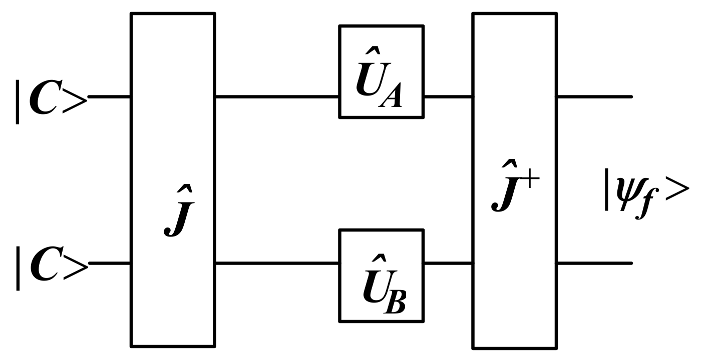
This study contains the following innovations: (1) it proposes an improved L–V model using quantum game theory to investigate population dynamics in an open system, putting aside the assumptions of two ecological competitors, two choices and independent strategies as in the Lotka–Volterra model; (2) In comparison with previous studies using the L–V model, such as Novak et al. [14,15], our proposed model exhibits swapping information and state superposition. Swapping information refers to non-revealed and continuous random information, which represent strategy interactions [34,35,36], such as learning from participating in repeated games, influenced by the amount of disposable information [37]. The game state is superposed in our model rather than mixed, and thus can be denoted by a qubit or tensor products of multiple qubits. State superposition means that all possible measurement values have some potential of being expressed at each moment, during which the potentials can interfere with each other—for example, wave interference can change the final observed measurement value [38]. State superposition is a basic trait of quantum computation and intrinsically represents the conflict, ambiguity, or uncertainty that people experience, as in the most famous example of Schrödinger’s cat “before the box is opened, the cat has two characteristics: death and life;” (3) Our method is similar to methods for investigating population dynamics using the evolutionary game model and L–V model theory, which considered mutual learning in repetitive games. However, our method differs in three important aspects. First, strategy interactions are considered in our model, rather than assuming that strategies are simply independent [3]. Second, our model considers the initial strategy state, which is ignored in the extant literature for population dynamics [39,40]. Third, the environmental capacity is regarded as dynamic in an open system in our model, unlike in the extant literature where environmental capacity was constant [9].

2. Theoretical Framework

2.1. Quantum Game Model

This section provides a brief summary of basic definitions and concepts from quantum game theory for readers who are new to quantum mechanics so that they can make sense of the theory. Although some readers might find quantum game theory to be completely new, the following brief explanation only emphasizes how to reach the concepts of strategy interaction and player strategy state. In this section, game players refer to two groups: player A and player B.

2.1.1. Basics of the Quantum Game Model

Quantum mechanics is arguably the most important and best empirically confirmed scientific theory in human history (Busemeyer and Wang, 2015). The quantum game model combines physical behavior information from quantum mechanics with game theory to describe swapping information between players and fulfilments. The evolution of the quantum system can be pictured through unitary matrices and, if considering the game of players and available strategies as qubits, the expression of the quantum system can be symbolized as $G\left(n,\Theta \left(H\right),\rho ,S,u\right)$ [41]. Here, $n$, $H$, $\Theta \left(H\right)$ are the number of races, Hilbert spaces and game state spaces, respectively; $\rho \in \Theta \left(H\right)$ is the initial quantum state; $S=S_1\times S_2\times \cdots \times S_n$ are strategy spaces; and $u=u_1\times u_2\times \cdots \times u_n$ is a utility function with $u_i:\Theta \left(H\right)\to \hslash$ for player $i$. In this study, for simplicity, any element or vector of the space of states is expressed by the symbol $\left|\cdot \right.〉$ (ket-vector) and $\left.〈\cdot \right|$ (bra-vector).

2.1.2. Hilbert Spaces and Space of States

A player faces a variety of strategies, while game payoffs are concrete realizations of those strategies. Let $\left\{\left|s_i\right.〉\right\}$ be the representation basis formed by the set of the basic representation states $\left|s_i\right.〉$. The representation basis is orthonormal and the strategy space $H_i\equiv \overline{U}\left\{\left|s_i\right.〉\right\}$ is the closed linear envelope of the representation basis, such that we have defined a Hilbert space. The strategy state can be expanded in terms of that basis as $\left|\psi \right.〉={\displaystyle \sum _{s_i}{c}_{s_i}}\left|S_i\right.〉$. Here, the strategy state is normalized such that $\left|〈S|S〉\right|=1$, and ${\displaystyle \sum _{s_i}{\left|c_{s_i}\right|}^2=}1$.

A set of several strategies is called a prospect and a prospect-representation is a concrete implementation of a prospect. The prospect-representation state is the tensor product of the representation states. It can be expressed as $\left|S\right.〉=\otimes \left|S_i\right.〉=\left|s_1{s}_2{s}_3\right.〉$, and the prospect-representation basis $\left|S\right.〉$ is also orthonormal, $〈S|S〉={\displaystyle \prod _{i,j}〈S_i|S_j〉}$, $〈S|S〉$ is the representation of inner product for $\left|S\right.〉$. The closed linear envelope of the prospect-representation state defines the prospect-space, which is a Hilbert space obtained as the tensor product of the strategy spaces, $H=\overline{U}\left\{\left|S\right.〉\right\}=\underset{i}{\otimes }{H}_i$.

2.1.3. Entanglement and Disentanglement

The literature from the quantum information and quantum computation fields emphasize the parameters related to entanglement measures. Considering interactions to be between actions available for a player and their beliefs about the other player, deviations from classical results arise from the interaction between the space of strategies of the two different players by a unitary operation; entanglement is such phenomenon that the global states of a composite system cannot be expressed by a product of the states of individual subsystems, which underlines the intrinsic order of statistical relations between subsystems of a compound quantum system [42]. Thus, a disentangled prospect-state is a prospect-state that can be expressed as $\left|\psi \right.〉=\underset{i}{\otimes }\left|{\psi }_i\right.〉$, which shows that the tensor product of strategy states $\left|\psi \right.〉$ can be decomposed. Thus, an entangled prospect-state is any prospect-state, $\left|\psi \right.〉\in H$, given by $\left|\psi \right.〉={\displaystyle \sum _S{c}_S}\left|S\right.〉$ and ${\displaystyle \sum _S{\left|c_S\right|}^2}=1$, which means a state $\left|\psi \right.〉$ is entangled if such a decomposition does not exist.

2.2. Calculation Steps for the Quantum Game Model

According to Sun [42] and Eisert [32], the basic calculation process for a quantum game can be illustrated as in Figure 1. The calculations include three steps: the initial quantum strategy state calculation, the final quantum strategy state calculation, and the quantum strategy-representation calculation. In this study, we assign the players’ payoffs directly as the strategy-representation of the concrete realization of the strategy according to classical decision-making theories.

2.2.1. Hypothesis

Before calculating the quantum strategy payoff, it is necessary to set the following hypothesis based on the characteristics of interdependent strategies in an open system.

Rule 1: Two group players (player A and player B), both have two basic vectors as Cooperation ($\widehat{C}$) and Competition ($\widehat{D}$). Importantly, the strategies of player A and player B are inter-dependent.

Rule 2: Both group players’ information can be simultaneously known by each other due to strategy entanglement.

Based on the above rules, the quantum payoffs matrix of basis vectors between player A and player B, can be expressed as shown in

Table 1. Basis vector game payoffs.

		Player B
		Cooperation ($\widehat{\mathit{C}}$)	Competition ($\widehat{\mathit{D}}$)
Player A	Cooperation ($\widehat{\mathit{C}}$)	$A_{11}$, $B_{11}$	$A_{12}$, $B_{12}$
	Competition ($\widehat{\mathit{D}}$)	$A_{21}$, $B_{21}$	$A_{22}$, $B_{22}$

. In Table 1, $A_{ij},B_{ij} \left(i,j=1,2\right)$ means the profit gained by player A and player B on the condition that player A chooses $i$ ($i$ = 1, Cooperation ($\widehat{C}$); $i$ = 2, Competition ($\widehat{D}$)) strategy, and player B chooses $j$ ($j$ = 1, Cooperation ($\widehat{C}$); $j$ = 2, Competition ($\widehat{D}$)) strategy simultaneously, respectively. All the parameters are positive.

2.2.2. Calculation Steps

Step 1: Calculate the initial quantum strategy state ($\left|{\psi }_i\right.〉$)

Payoffs of the quantum game rely on potential outputs from classical strategies. Assuming that the classical available strategies for both players in this game are $D$ and $C$, we assign as two fundamental vectors $\left|C\right.〉=\left(\begin{array}{c}1\\ 0\end{array}\right)$, $\left|D\right.〉=\left(\begin{array}{c}0\\ 1\end{array}\right)$, each representing a qubit, respectively, to the basis of the Hilbert space. Considering the Hilbert space given by the tensor product of spaces associated with each player’s strategy and their evaluation of what the other player will choose, the starting strategy state can be spanned by any combination of four bases $\left|CC\right.〉$, $\left|CD\right.〉$, $\left|DC\right.〉$, $\left|DD\right.〉$. Next, the qubits $\left|C\right.〉\otimes \left|D\right.〉$ go through a two-qubit entangling gate $\widehat{J}=\exp \left(i\gamma \widehat{D}\otimes \widehat{D}/2\right)$, which is a reversible two-bit gate with entanglement parameter $\gamma \in \left[0,\raisebox{1ex}{$\pi $}\!\left/ \!\raisebox{-1ex}{$2$}\right.\right]$. Then, the quantization process of the game can be represented as Equation (3).

$$\widehat{J}=\exp \left(i\gamma \widehat{D}\otimes \widehat{D}/2\right)=\exp \left(i\raisebox{1ex}{$\gamma $}\!\left/ \!\raisebox{-1ex}{$2$}\right.\left(\begin{array}{cc}0& 1\\ -1& 0\end{array}\right)\otimes \left(\begin{array}{cc}0& 1\\ -1& 0\end{array}\right)\right)=\left(\begin{array}{cccc}\cos \left(\raisebox{1ex}{$\gamma $}\!\left/ \!\raisebox{-1ex}{$2$}\right.\right)& 0& 0& i \sin \left(\raisebox{1ex}{$\gamma $}\!\left/ \!\raisebox{-1ex}{$2$}\right.\right)\\ 0& \cos \left(\raisebox{1ex}{$\gamma $}\!\left/ \!\raisebox{-1ex}{$2$}\right.\right)& -i \sin \left(\raisebox{1ex}{$\gamma $}\!\left/ \!\raisebox{-1ex}{$2$}\right.\right)& 0\\ 0& -i \sin \left(\raisebox{1ex}{$\gamma $}\!\left/ \!\raisebox{-1ex}{$2$}\right.\right)& \cos \left(\raisebox{1ex}{$\gamma $}\!\left/ \!\raisebox{-1ex}{$2$}\right.\right)& 0\\ i \sin \left(\raisebox{1ex}{$\gamma $}\!\left/ \!\raisebox{-1ex}{$2$}\right.\right)& 0& 0& \cos \left(\raisebox{1ex}{$\gamma $}\!\left/ \!\raisebox{-1ex}{$2$}\right.\right)\end{array}\right).$$

(3)

Subsequently, the initial quantum strategy state can be obtained from Equation (4)

$$\left|{\psi }_i\right.〉=\widehat{J}\left|CD\right.〉=\left(\begin{array}{c}0\\ \cos \left(\raisebox{1ex}{$\gamma $}\!\left/ \!\raisebox{-1ex}{$2$}\right.\right)\\ -i \sin \left(\raisebox{1ex}{$\gamma $}\!\left/ \!\raisebox{-1ex}{$2$}\right.\right)\\ 0\end{array}\right).$$

(4)

Here, parameter $\gamma$ is the game’s entanglement parameter if $\gamma =0$ means a separable game; $\left|{\psi }_i\right.〉$ is the initial state.

Step 2: Calculate the final quantum strategy state ($\left|{\psi }_f\right.〉$)

${\widehat{U}}_A$ and ${\widehat{U}}_B$ are local unitary operators for the local manipulation of player A and player B, respectively. A pure quantum strategy $\widehat{U}\left(\theta ,\alpha \right)$ is a special unitary group $SU(2)$ operator, which can be described by Equation (5).

$$\widehat{U}\left(\theta ,\alpha \right)=\left(\begin{array}{cc}{e}^{i\alpha }\cos \left(\theta /2\right)& \sin \left(\theta /2\right)\\ -\sin \left(\theta /2\right)& e^{-i\alpha }\cos \left(\theta /2\right)\end{array}\right),$$

(5)

where $0\le \theta \le \pi$ and $0\le \alpha \le \raisebox{1ex}{$\pi $}\!\left/ \!\raisebox{-1ex}{$2$}\right.$; the operators of the cooperation and competition strategies are $\widehat{C}\equiv \widehat{U}\left(0,0\right)$ and $\widehat{D}\equiv \widehat{U}\left(\pi ,0\right)$, respectively.

Once players carry out their actions, their game is turned into state $\left({\widehat{U}}_A\otimes {\widehat{U}}_B\right)\widehat{J}\left|CD\right.〉$, and the two group players propose their qubits for the final measurement, which is achieved by a gate reversible $\tilde{J}={\widehat{J}}^{+}$. The final state ($\left|{\psi }_f\right.〉$) is a superposition as shown in Equations (6) and (7).

$$\left|{\psi }_f\right.〉=\tilde{J}\left({\widehat{U}}_A\otimes {\widehat{U}}_B\right)\widehat{J}\left|CD\right.〉$$

(6)

$${\widehat{U}}_A\otimes {\widehat{U}}_B=\left(\begin{array}{cc}{e}^{i{\alpha }_A}\cos \left({\theta }_A/2\right)& \sin \left({\theta }_A/2\right)\\ -\sin \left({\theta }_A/2\right)& e^{-i{\alpha }_A}\cos \left({\theta }_A/2\right)\end{array}\right)\otimes \left(\begin{array}{cc}{e}^{i{\alpha }_B}\cos \left({\theta }_B/2\right)& \sin \left({\theta }_B/2\right)\\ -\sin \left({\theta }_B/2\right)& e^{-i{\alpha }_B}\cos \left({\theta }_B/2\right)\end{array}\right).$$

(7)

Accordingly,

$$\begin{array}{cc}\hfill & \left|\psi {}_f\right.〉=\tilde{J}\left({\widehat{U}}_A\otimes {\widehat{U}}_B\right)\widehat{J}\left|CD\right.〉\hfill \\ \hfill & =\left(\begin{array}{c}cos\left({\theta }_A/2\right)cos\left({\theta }_B/2\right)cos\left({\alpha }_A\right)+sin\left({\theta }_A/2\right)cos\left({\theta }_B/2\right)sin\left({\alpha }_B\right)sin\left(\gamma \right)+icos\left({\theta }_A/2\right)sin\left({\theta }_B/2\right)sin\left({\alpha }_A\right)cos\left(\gamma \right)\\ cos\left({\theta }_A/2\right)cos\left({\theta }_B/2\right)\left(cos\left({\alpha }_A-{\alpha }_B\right)-icos\left({\alpha }_A-{\alpha }_B\right)sin\left(\gamma \right)\right)\\ cos\left({\theta }_A/2\right)cos\left({\theta }_B/2\right)cos\left({\alpha }_A\right)sin\left({\alpha }_B\right)sin\left(\gamma \right)-sin\left({\theta }_A/2\right)sin\left({\theta }_B/2\right)-cos\left({\theta }_A/2\right)cos\left({\theta }_B/2\right)sin\left({\alpha }_A\right)cos\left({\alpha }_B\right)sin\left(\gamma \right)\\ cos\left({\theta }_A/2\right)sin\left({\theta }_B/2\right)sin\left({\alpha }_A\right)sin\left(\gamma \right)-sin\left({\theta }_A/2\right)cos\left({\theta }_B/2\right)cos\left({\alpha }_B\right)+isin\left({\theta }_A/2\right)cos\left({\theta }_B/2\right)sin\left({\alpha }_B\right)cos\left(\gamma \right)\end{array}\right)\hfill \end{array}.$$

(8)

The measurement of Equation (8) will cause the final state to collapse into one of the classical outcomes, and a payoff is obtained in line with the corresponding matrix entries.

Step 3: Calculate quantum payoffs

Considering the computing example of payoffs in a quantum game [42,43], one player’s quantum payoff (${\overline{\$}}_A$) can be defined as Equation (9). Then, according to Equation (8) the probability of the final state collapsing into the basis vector of the tensor product space is calculated as Equation (10). Finally, the quantum payoff of the entangled quantum game can be calculated by integrating Equations (9) and (10).

$$\left\{\begin{array}{l}{\overline{\mathit{\$}}}_A=A_{11}{P}_{CC}+A_{12}{P}_{CD}+A_{21}{P}_{DC}+A_{22}{P}_{DD}\\ P_{CC}={\left|\left.〈C{C}^{\prime }\right|{\psi }_f〉\right|}^2\\ P_{CD}={\left|\left.〈C{D}^{\prime }\right|{\psi }_f〉\right|}^2\\ P_{DC}={\left|\left.〈D{C}^{\prime }\right|{\psi }_f〉\right|}^2\\ P_{DD}={\left|\left.〈D{D}^{\prime }\right|{\psi }_f〉\right|}^2\end{array}\right.,$$

(9)

$$\left\{\begin{array}{c}{P}_{CC}={\left(cos\left({\theta }_A/2\right)cos\left({\theta }_B/2\right)cos\left({\alpha }_A\right)+sin\left({\theta }_A/2\right)cos\left({\theta }_B/2\right)sin\left({\alpha }_B\right)sin\left(\gamma \right)\right)}^2-{\left(cos\left({\theta }_A/2\right)sin\left({\theta }_B/2\right)sin\left({\alpha }_A\right)cos\left(\gamma \right)\right)}^2\hfill \\ P_{CD}={cos}^2\left({\theta }_A/2\right){cos}^2\left({\theta }_B/2\right)\left({cos}^2\left({\alpha }_A-{\alpha }_B\right)+{cos}^2\left({\alpha }_A-{\alpha }_B\right){sin}^2\left(\gamma \right)\right)\hfill \\ P_{DC}={\left(cos\left({\theta }_A/2\right)cos\left({\theta }_B/2\right)cos\left({\alpha }_A\right)sin\left({\alpha }_B\right)sin\left(\gamma \right)-sin\left({\theta }_A/2\right)sin\left({\theta }_B/2\right)-cos\left({\theta }_A/2\right)cos\left({\theta }_B/2\right)sin\left({\alpha }_A\right)cos\left({\alpha }_B\right)sin\left(\gamma \right)\right)}^2\hfill \\ P_{DD}={\left(cos\left({\theta }_A/2\right)sin\left({\theta }_B/2\right)sin\left({\alpha }_A\right)sin\left(\gamma \right)-sin\left({\theta }_A/2\right)cos\left({\theta }_B/2\right)cos\left({\alpha }_B\right)\right)}^2-{\left(sin\left({\theta }_A/2\right)cos\left({\theta }_B/2\right)sin\left({\alpha }_B\right)cos\left(\gamma \right)\right)}^2\hfill \end{array}\right.,$$

(10)

where $P_{CC}$, $P_{CD}$, $P_{DC}$, $P_{DD}$ are the probabilities of the final quantum strategy state collapsing into pure outcomes $\left|C{C}^{\prime }\right.〉$, $\left|C{D}^{\prime }\right.〉$, $\left|D{C}^{\prime }\right.〉$, $\left|D{D}^{\prime }\right.〉$, respectively. Equations (9) and (10) show that quantum payoffs can be expressed by traditional game payoffs and the entanglement parameter $\gamma$ considering the parameters of each player’s strategic evolution.

3. An Improved L–V Model: Coexistence of Competition and Cooperation

This part focuses on equilibrium analysis of the improved L–V model, based on part two, which explains and describes the computation process of the quantum game. Firstly, based on the interaction parameters, each player’s interactive coexistence can be classified as either cooperative or competitive [8]. Cooperative coexistence means that the interactive parameters are positive, while competitive coexistence has negative interactive parameters. Thus, an improved coexistence model integrating density game theory and quantum decision making can be expressed as Equation (11) for competition coexistence and Equation (12) for cooperation coexistence. Then, based on the three payoff calculation steps for the quantum game and related equations, six special cases can be obtained (

Table 2. Quantum payoffs by case.

Case	Strategy	Parameter	Quantum Payoff
1	${\widehat{U}}_A=\widehat{Q}$, ${\widehat{U}}_B=\widehat{Q}$	${\theta }_A=0$, ${\theta }_B=0$, ${\alpha }_A=\raisebox{1ex}{$\pi $}\!\left/ \!\raisebox{-1ex}{$2$}\right.$,${\alpha }_B=\raisebox{1ex}{$\pi $}\!\left/ \!\raisebox{-1ex}{$2$}\right.$	$\overline{R_A}=A_{11}$, $\overline{R_B}=B_{11}$
2	${\widehat{U}}_A=\widehat{C}$, ${\widehat{U}}_B=\widehat{Q}$	${\theta }_A=0$, ${\theta }_B=0$, ${\alpha }_A=0$, ${\alpha }_B=\raisebox{1ex}{$\pi $}\!\left/ \!\raisebox{-1ex}{$2$}\right.$	$\overline{R_A}=A_{11}+\left(A_{22}-A_{11}\right){\sin }^2\left(\gamma \right)$, $\overline{R_B}=B_{11}+\left(B_{22}-B_{11}\right){\sin }^2\left(\gamma \right)$
3	${\widehat{U}}_A=\widehat{D}$, ${\widehat{U}}_B=\widehat{Q}$	${\theta }_A=\pi$, ${\theta }_B=0$, ${\alpha }_A=0$, ${\alpha }_B=\raisebox{1ex}{$\pi $}\!\left/ \!\raisebox{-1ex}{$2$}\right.$	$\overline{R_A}=A_{21}+\left(A_{12}-A_{21}\right){\sin }^2\left(\gamma \right)$, $\overline{R_B}=B_{21}+\left(B_{12}-B_{21}\right){\sin }^2\left(\gamma \right)$
4	${\widehat{U}}_A=\widehat{D}$, ${\widehat{U}}_B=\widehat{D}$	${\theta }_A=\pi$, ${\theta }_B=\pi$, ${\alpha }_A=0$, ${\alpha }_B=0$	$\overline{R_A}=A_{22}$, $\overline{R_B}=B_{22}$
5	${\widehat{U}}_A=\widehat{C}$, ${\widehat{U}}_B=\widehat{C}$	${\theta }_A=0$, ${\theta }_B=0$, ${\alpha }_A=0$, ${\alpha }_B=0$	$\overline{R_A}=A_{11}$, $\overline{R_B}=B_{11}$
6	${\widehat{U}}_A=\widehat{D}$, ${\widehat{U}}_B=\widehat{C}$	${\theta }_A=\pi$, ${\theta }_B=0$, ${\alpha }_A=0$, ${\alpha }_B=0$	$\overline{R_A}=A_{21}$, $\overline{R_B}=B_{21}$

(Note: $\overline{R_A}$, $\overline{R_B}$, player A’s and player B’s payoff, respectively).

).

$$\left\{\begin{array}{c}\frac{d{x}_A}{dt}=r_A{x}_A\left(1-\frac{x_B}{\overline{R_B}{M}_B}-\frac{x_A}{M_A}\right)\\ \frac{d{x}_B}{dt}=r_B{x}_B\left(1-\frac{x_B}{M_B}-\frac{x_A}{\overline{R_A}{M}_A}\right)\end{array}\right.$$

(11)

$$\left\{\begin{array}{c}\frac{d{x}_A}{dt}=r_A{x}_A\left(1+\frac{x_B}{\overline{R_B}{M}_B}-\frac{x_A}{M_A}\right)\\ \frac{d{x}_B}{dt}=r_B{x}_B\left(1-\frac{x_B}{M_B}+\frac{x_A}{\overline{R_A}{M}_A}\right)\end{array}\right.,$$

(12)

where $x_A$ is the population size of player A; $M_A$ represents the maximum environmental capacity for player A; $r_A$ denotes net natural growing rate for player A; $\overline{R_A}$, $\overline{R_B}$, are the quantum average payoffs for players A and B, respectively; $\overline{R_A}$, $\overline{R_B}$ represent mutual effect coefficients for the players; $\overline{R_A}{M}_A$, $\overline{R_B}{M}_B$, are the maximum gains for player A and player B under the maximum environmental capacity, respectively. $r_B{x}_B$, $r_A{x}_A$, reflects each players’ developing trends. $1-\frac{x_A}{M_A}$, $1-\frac{x_B}{M_B}$, are the coefficients of damped growth, stemming from the environmental capacities of player A and player B, respectively.

In Table 2, case 1 illustrates when both players initially take the same quantum strategy ${\widehat{U}}_A={\widehat{U}}_B=\widehat{U}\left(0, \raisebox{1ex}{$\pi $}\!\left/ \!\raisebox{-1ex}{$2$}\right.\right)=\widehat{Q}=\left(\begin{array}{cc}i& 0\\ 0& -i\end{array}\right)$, taking their competitor’s strategy into account (i.e., the largest entanglement intensity $\gamma =\frac{\pi }{2}$). Case 2 is when initially player A selects the cooperative strategy ${\widehat{U}}_A=\widehat{U}\left(0, 0\right)=\widehat{C}$, ignoring the strategy of player B, while player B selects quantum strategy ${\widehat{U}}_B=\widehat{U}\left(0, \raisebox{1ex}{$\pi $}\!\left/ \!\raisebox{-1ex}{$2$}\right.\right)=\widehat{Q}$, taking the strategy of player A into account. Case 3 illustrates when the initial strategy of player A is the Competitive strategy ${\widehat{U}}_A=\widehat{U}\left(0, 0\right)=\widehat{D}$, ignoring the strategy of player B, but player B initially selects ${\widehat{U}}_B=\widehat{U}\left(0, \raisebox{1ex}{$\pi $}\!\left/ \!\raisebox{-1ex}{$2$}\right.\right)=\widehat{Q}$, taking the strategy of player A into account. Cases 4–6 show both players implementing pure and independent strategies as in the classical game model. Thus, the following sections focus on the cases 1–3 since they cover cases not in the classical game model.

3.1. Equilibrium and Stability Conditions in Competitive Coexistence

According to the stability theory of ordinary differential equations, in Equation (11), four local equilibriums can be obtained as $E_1\left(0,0\right)$, $E_2\left(0,M_B\right)$, $E_3\left(M_A,0\right)$, and $E_4\left(\frac{M_A\overline{R_A}\left(\overline{R_B}-1\right)}{\overline{R_A}\overline{R_B}-1},\frac{M_B\overline{R_B}\left(\overline{R_A}-1\right)}{\overline{R_A}\overline{R_B}-1}\right)$. Comparing the four local equilibrium points, $E_4$ means that players are coexisting while $\mathrm{sgn}\left(\overline{R_A}\overline{R_B}-1\right)$ = $\mathrm{sgn}\left(\overline{R_B}-1\right)$ = $\mathrm{sgn}\left(\overline{R_A}-1\right)=+1$ or $-1$. Then, based upon the stability theory of ordinary differential equations, the Jacobean matrix of Equation (11) can be expressed as Equation (13). The corresponding determinant value and trace of the matrix can be expressed as in Equation (14).

$$J=\left[\begin{array}{cc}{r}_A-\frac{r_A{x}_B}{M_B\overline{R_B}}-\frac{2r_A{x}_A}{M_A}& -\frac{r_A{x}_A}{M_B\overline{R_B}}\\ -\frac{r_B{x}_B}{M_A\overline{R_A}}& r_B-\frac{r_B{x}_A}{M_A\overline{R_A}}-\frac{2r_B{x}_B}{M_B}\end{array}\right]$$

(13)

$$\left\{\begin{array}{l}\det J=\left(r_A-\frac{r_A{x}_B}{M_B\overline{R_B}}-\frac{2r_A{x}_A}{M_A}\right)*\left(r_B-\frac{r_B{x}_A}{M_A\overline{R_A}}-\frac{2r_B{x}_B}{M_B}\right)-\frac{r_A{x}_A}{M_B\overline{R_B}}*\frac{r_B{x}_B}{M_A\overline{R_A}}\\ trJ=-\left[\left(r_A-\frac{r_A{x}_B}{M_B\overline{R_B}}-\frac{2r_A{x}_A}{M_A}\right)+\left(r_B-\frac{r_B{x}_A}{M_A\overline{R_A}}-\frac{2r_B{x}_B}{M_B}\right)\right]\end{array}\right..$$

(14)

Then, according to the stability theory of ordinary differential equations, the equilibrium reaches the asymptotic stable state when $trJ>0$ and $\det J>0$. The determinant symbol, trace symbol and the stability condition of the equilibrium points in competition coexistence can be obtained as shown in

Table 3. Stability analysis of coexistence equilibrium in the competition symbiosis.

Equilibrium	$\mathbf{det}\mathit{J}$	$\mathit{t}\mathit{r}\mathit{J}$	Stability Condition
$E_4\left(\frac{M_A\overline{R_A}\left(\overline{R_B}-1\right)}{\overline{R_A}\overline{R_B}-1},\frac{M_B\overline{R_B}\left(\overline{R_A}-1\right)}{\overline{R_A}\overline{R_B}-1}\right)$	$\frac{r_A{r}_A\left(\overline{R_A}-1\right)\left(\overline{R_B}-1\right)}{\overline{R_A}\overline{R_B}-1}$	$\frac{\overline{R_A}{r}_A\left(\overline{R_B}-1\right)+\overline{R_B}{r}_B\left(\overline{R_A}-1\right)}{\overline{R_A}\overline{R_B}-1}$	$\mathrm{sgn}\left(\overline{R_A}\overline{R_B}-1\right)$ = $\mathrm{sgn}\left(\overline{R_B}-1\right)$ = $\mathrm{sgn}\left(\overline{R_A}-1\right)$$=+1$

. Here, $E_4$ has a coexisting state when $\mathrm{sgn}\left(\overline{R_A}\overline{R_B}-1\right)$ = $\mathrm{sgn}\left(\overline{R_B}-1\right)$ = $\mathrm{sgn}\left(\overline{R_A}-1\right)=+1$, and the population scales of the two players are positive. Here, $\overline{R_B}$, $\overline{R_A}$ are payoff functions for players B and A, respectively, combining the matrix payoff items with their entanglement parameters. Then, the equilibrium and stability conditions in cases 1–3 (

Table 4. Stability conditions for coexistence equilibrium by case for the competition scenario.

Case	Equilibrium	Stability Condition
1	${\mathit{E}}_4\left(\frac{{\mathit{M}}_{\mathit{A}}{\mathit{A}}_{11}\left({\mathit{B}}_{11}-1\right)}{{\mathit{A}}_{11}{\mathit{B}}_{11}-1},\frac{{\mathit{M}}_{\mathit{B}}{\mathit{B}}_{11}\left({\mathit{A}}_{11}-1\right)}{{\mathit{A}}_{11}{\mathit{B}}_{11}-1}\right)$	$\mathbf{sgn}\left({\mathit{A}}_{11}{\mathit{B}}_{11}-1\right)=\mathbf{sgn}\left({\mathit{A}}_{11}-1\right)=\mathbf{sgn}\left({\mathit{B}}_{11}-1\right)=+1$
2	$E_4\left(\begin{array}{l}\frac{M_A\left(A_{11}+\left(A_{22}-A_{11}\right){\sin }^2\left(\gamma \right)\right)\left(\left(B_{11}+\left(B_{22}-B_{11}\right){\sin }^2\left(\gamma \right)\right)-1\right)}{\left(A_{11}+\left(A_{22}-A_{11}\right){\sin }^2\left(\gamma \right)\right)\left(B_{11}+\left(B_{22}-B_{11}\right){\sin }^2\left(\gamma \right)\right)-1},\\ \frac{M_B\left(B_{11}+\left(B_{22}-B_{11}\right){\sin }^2\left(\gamma \right)\right)\left(\left(A_{11}+\left(A_{22}-A_{11}\right){\sin }^2\left(\gamma \right)\right)-1\right)}{\left(A_{11}+\left(A_{22}-A_{11}\right){\sin }^2\left(\gamma \right)\right)\left(B_{11}+\left(B_{22}-B_{11}\right){\sin }^2\left(\gamma \right)\right)-1}\end{array}\right)$	$\begin{array}{l}\mathrm{sgn}\left(\left(A_{11}+\left(A_{22}-A_{11}\right){\sin }^2\left(\gamma \right)\right)\left(B_{11}+\left(B_{22}-B_{11}\right){\sin }^2\left(\gamma \right)\right)-1\right)\\ =\mathrm{sgn}\left(A_{11}+\left(A_{22}-A_{11}\right){\sin }^2\left(\gamma \right)-1\right)\\ =\mathrm{sgn}\left(B_{11}+\left(B_{22}-B_{11}\right){\sin }^2\left(\gamma \right)-1\right)=+1\end{array}$
3	$E_4\left(\begin{array}{l}\frac{M_A\left(A_{21}+\left(A_{12}-A_{21}\right){\sin }^2\left(\gamma \right)\right)\left(\left(B_{12}+\left(B_{21}-B_{12}\right){\sin }^2\left(\gamma \right)\right)-1\right)}{\left(A_{21}+\left(A_{12}-A_{21}\right){\sin }^2\left(\gamma \right)\right)\left(B_{12}+\left(B_{21}-B_{12}\right){\sin }^2\left(\gamma \right)\right)-1},\\ \frac{M_B\left(B_{12}+\left(B_{21}-B_{12}\right){\sin }^2\left(\gamma \right)\right)\left(\left(A_{21}+\left(A_{12}-A_{21}\right){\sin }^2\left(\gamma \right)\right)-1\right)}{\left(A_{21}+\left(A_{12}-A_{21}\right){\sin }^2\left(\gamma \right)\right)\left(B_{12}+\left(B_{21}-B_{12}\right){\sin }^2\left(\gamma \right)\right)-1}\end{array}\right)$	$\begin{array}{l}\mathrm{sgn}\left(\left(A_{21}+\left(A_{12}-A_{21}\right){\sin }^2\left(\gamma \right)\right)\left(B_{12}+\left(B_{21}-B_{12}\right){\sin }^2\left(\gamma \right)\right)-1\right)\\ =\mathrm{sgn}\left(\left(\left(B_{12}+\left(B_{21}-B_{12}\right){\sin }^2\left(\gamma \right)\right)-1\right)\right)\\ =\mathrm{sgn}\left(\left(\left(A_{21}+\left(A_{12}-A_{21}\right){\sin }^2\left(\gamma \right)\right)-1\right)\right)=+1\end{array}$

) can be obtained as shown in Table 4.

In addition, on the basis of the stability condition $\mathrm{sgn}\left(\overline{R_A}\overline{R_B}-1\right)$ = $\mathrm{sgn}\left(\overline{R_B}-1\right)$ = $\mathrm{sgn}\left(\overline{R_A}-1\right)=+1$ (Table 4), if $\mathrm{sgn}\left(\overline{R_B}-1\right)$ = $\mathrm{sgn}\left(\overline{R_A}-1\right)=+1$ is met, then $\mathrm{sgn}\left(\overline{R_A}\overline{R_B}-1\right)=+1$ should also be naturally met. According to the stability conditions of cases 1 and 3, their interactive intensity $\gamma \in \left[0,\raisebox{1ex}{$\pi $}\!\left/ \!\raisebox{-1ex}{$2$}\right.\right]$, is a quantum entanglement parameter meeting the stability condition, which can be obtained as one of the cases in Equation (15).

$$\left\{\begin{array}{l}Case 1: \gamma \in \left[0,\frac{\pi }{2}\right]\\ \\ Case 2:{\sin }^2\gamma <\min \left(\raisebox{1ex}{$\left(A_{11}-1\right)$}\!\left/ \!\raisebox{-1ex}{$\left(A_{11}-A_{22}\right)$}\right.,\raisebox{1ex}{$\left(B_{11}-1\right)$}\!\left/ \!\raisebox{-1ex}{$\left(B_{11}-B_{22}\right)$}\right.\right)\\ \\ \mathrm{Case} 3: {\sin }^2\gamma <\min \left(\raisebox{1ex}{$\left(B_{21}-1\right)$}\!\left/ \!\raisebox{-1ex}{$\left(B_{21}-B_{12}\right)$}\right.,\raisebox{1ex}{$\left(A_{21}-1\right)$}\!\left/ \!\raisebox{-1ex}{$\left(A_{21}-A_{12}\right)$}\right.\right)\end{array}\right.$$

(15)

3.2. Equilibrium and Stability Conditions in Cooperative Coexistence

According to the stability theory of ordinary differential equations, Equation (12) can reach four local equilibriums: $E_1\left(0,0\right)$, $E_2\left(0,M_B\right)$, $E_3\left(M_A,0\right)$, and $E_4\left(\frac{M_A\overline{R_A}\left(\overline{R_B}+1\right)}{\overline{R_A}\overline{R_B}-1},\frac{M_B\overline{R_B}\left(\overline{R_A}+1\right)}{\overline{R_A}\overline{R_B}-1}\right)$. Based on $\mathrm{sgn}\left(\overline{R_A}\overline{R_B}-1\right)=+1$, the equilibrium state in $E_4$ is the coexistence equilibrium with positive population growth for both players. The Jacobean matrix of the equation can be obtained as Equation (16). Then, the related determinant value and trace of the matrix can be calculated based on Equation (16), and the calculation result is shown in Equation (17).

$$J=\left[\begin{array}{cc}{r}_A+\frac{r_A{x}_B}{M_B\overline{R_B}}-\frac{2r_A{x}_A}{M_A}& \frac{r_A{x}_A}{M_B\overline{R_B}}\\ \frac{r_B{x}_B}{M_A\overline{R_A}}& r_B+\frac{r_B{x}_A}{M_A\overline{R_A}}-\frac{2r_B{x}_B}{M_B}\end{array}\right]$$

(16)

$$\left\{\begin{array}{l}\det J=\left(r_A+\frac{r_A{x}_B}{M_B\overline{R_B}}-\frac{2r_A{x}_A}{M_A}\right)*\left(r_B+\frac{r_B{x}_A}{M_A\overline{R_A}}-\frac{2r_B{x}_B}{M_B}\right)-\frac{r_A{x}_A}{M_B\overline{R_B}}*\frac{r_B{x}_B}{M_A\overline{R_A}}\\ trJ=-\left[\left(r_A+\frac{r_A{x}_B}{M_B\overline{R_B}}-\frac{2r_A{x}_A}{M_A}\right)+\left(r_B+\frac{r_B{x}_A}{M_A\overline{R_A}}-\frac{2r_B{x}_B}{M_B}\right)\right]\end{array}\right.$$

(17)

Note that, according to the stability theory of ordinary differential equations, the equilibrium can evolve to the asymptotic stable state when $trJ>0$ and $\det J>0$. The determinant symbol, trace symbol and the stability condition of the equilibrium point in the cooperation scenario can be obtained as shown in

Table 5. Stability analysis of coexistence equilibrium in the cooperation symbiosis.

Equilibrium	$\mathbf{det}\mathit{J}$	$\mathit{t}\mathit{r}\mathit{J}$	Stability Condition
$E_4\left(\frac{M_A\overline{R_A}\left(\overline{R_B}+1\right)}{\overline{R_A}\overline{R_B}-1},\frac{M_B\overline{R_B}\left(\overline{R_A}+1\right)}{\overline{R_A}\overline{R_B}-1}\right)$	$\frac{r_A{r}_A\left(\overline{R_A}+1\right)\left(\overline{R_B}+1\right)}{\overline{R_A}\overline{R_B}-1}$	$\frac{\overline{R_A}{r}_A\left(\overline{R_B}+1\right)+\overline{R_B}{r}_B\left(\overline{R_A}+1\right)}{\overline{R_A}\overline{R_B}-1}$	$\mathrm{sgn}\left(\overline{R_A}\overline{R_B}-1\right)$$=+1$

. The coexistence point $E_4$ is stable when $\mathrm{sgn}\left(\overline{R_A}\overline{R_B}-1\right)=+1$, and population change is positive. Further, in view of cooperation coexistence and its stability condition (Table 5), the equilibrium and stability conditions of cases 1–3 (Table 3) are shown in

Table 6. Stability conditions for coexistence equilibrium by case for cooperation symbiosis.

Case	Equilibrium	Stability Condition
1	${\mathit{E}}_4\left(\frac{{\mathit{M}}_{\mathit{A}}{\mathit{A}}_{11}\left({\mathit{B}}_{11}+1\right)}{{\mathit{A}}_{11}{\mathit{B}}_{11}-1},\frac{{\mathit{M}}_{\mathit{B}}{\mathit{B}}_{11}\left({\mathit{A}}_{11}+1\right)}{{\mathit{A}}_{11}{\mathit{B}}_{11}-1}\right)$	$\mathbf{sgn}\left({\mathit{A}}_{11}{\mathit{B}}_{11}-1\right)$$=+1$
2	$E_4\left(\begin{array}{l}\frac{M_A\left(A_{11}+\left(A_{22}-A_{11}\right){\sin }^2\left(\gamma \right)\right)\left(\left(B_{11}+\left(B_{22}-B_{11}\right){\sin }^2\left(\gamma \right)\right)+1\right)}{\left(A_{11}+\left(A_{22}-A_{11}\right){\sin }^2\left(\gamma \right)\right)\left(B_{11}+\left(B_{22}-B_{11}\right){\sin }^2\left(\gamma \right)\right)-1},\\ \frac{M_B\left(B_{11}+\left(B_{22}-B_{11}\right){\sin }^2\left(\gamma \right)\right)\left(\left(A_{11}+\left(A_{22}-A_{11}\right){\sin }^2\left(\gamma \right)\right)+1\right)}{\left(A_{11}+\left(A_{22}-A_{11}\right){\sin }^2\left(\gamma \right)\right)\left(B_{11}+\left(B_{22}-B_{11}\right){\sin }^2\left(\gamma \right)\right)-1}\end{array}\right)$	$\begin{array}{l}\mathrm{sgn}\left(A_{11}+\left(A_{22}-A_{11}\right){\sin }^2\left(\gamma \right)\right)\left(B_{11}+\left(B_{22}-B_{11}\right){\sin }^2\left(\gamma \right)\right)-1\\ =+1\end{array}$
3	$E_4\left(\begin{array}{l}\frac{M_A\left(A_{21}+\left(A_{12}-A_{21}\right){\sin }^2\left(\gamma \right)\right)\left(\left(B_{12}+\left(B_{21}-B_{12}\right){\sin }^2\left(\gamma \right)\right)+1\right)}{\left(A_{21}+\left(A_{12}-A_{21}\right){\sin }^2\left(\gamma \right)\right)\left(B_{12}+\left(B_{21}-B_{12}\right){\sin }^2\left(\gamma \right)\right)-1},\\ \frac{M_B\left(B_{12}+\left(B_{21}-B_{12}\right){\sin }^2\left(\gamma \right)\right)\left(\left(A_{21}+\left(A_{12}-A_{21}\right){\sin }^2\left(\gamma \right)\right)+1\right)}{\left(A_{21}+\left(A_{12}-A_{21}\right){\sin }^2\left(\gamma \right)\right)\left(B_{12}+\left(B_{21}-B_{12}\right){\sin }^2\left(\gamma \right)\right)-1}\end{array}\right)$	$\begin{array}{l}\mathrm{sgn}\left(\left(A_{21}+\left(A_{12}-A_{21}\right){\sin }^2\left(\gamma \right)\right)\left(B_{12}+\left(B_{21}-B_{12}\right){\sin }^2\left(\gamma \right)\right)-1\right)\\ =+1\end{array}$

. Thus, according to the stability conditions of those cases, the range of entanglement parameters meeting the stability conditions can be calculated as for the cases in Equation (17).

4. Results and Scenario Analysis

Based on the improved L–V model proposed above and the calculated results of players’ strategy equilibrium and stability conditions, the simulation results for competition and cooperation coexistence are shown as follows (Table 3, Table 4, Table 5 and Table 6). In case 1, players implement the initial strategies with the largest entanglement intensity. First, in competitive coexistence, players’ strategies evolve into a state where the population sizes of the two players reach a stable state (player A: $\frac{M_A{A}_{11}(B_{11}-1)}{A_{11}{B}_{11}-1}$; player B: $\frac{M_B{B}_{11}(A_{11}-1)}{A_{11}{B}_{11}-1}$) once $\mathrm{sgn}(A_{11}{B}_{11}-1)=\mathrm{sgn}(A_{11}-1)=\mathrm{sgn}(B_{11}-1)=+1$ (Table 3 and Table 4). Second, in cooperative coexistence, the final and stable sizes of players’ populations are $\frac{M_A{A}_{11}(B_{11}+1)}{A_{11}{B}_{11}-1}$ (player A) and $\frac{M_B{B}_{11}(A_{11}+1)}{A_{11}{B}_{11}-1}$ (player B) once $\mathrm{sgn}(A_{11}{B}_{11}-1)=\mathrm{sgn}(A_{11}-1)=\mathrm{sgn}(B_{11}-1)=+1$ (Table 5 and Table 6). Case 1 simulation results reflect that the final and stable sizes of players’ populations are decided by their environmental capacity ($M_A$ and $M_B$) and payoffs ($A_{11}$ and $B_{11}$). It seems that players with larger environmental capacities or higher returns will obtain larger population sizes. In cases 2–3, in competitive (Table 3 and Table 4) and cooperative coexistence (Table 5 and Table 6), all players’ strategies finally evolve into a state with stable population sizes, when the entanglement intensity of strategy interaction meets the requirements illustrated in Equations (15). The results show that players’ population sizes are decided by their environmental capacities ($M_A$ and $M_B$), payoff items (Table 1) and entanglement intensity $\left(\gamma \right)$. Thus, the following analysis of scenarios further investigates the influences of entanglement intensity and payoffs in various settings for coexistence on the player population sizes using scenario simulations.

4.1. Scenario Settings

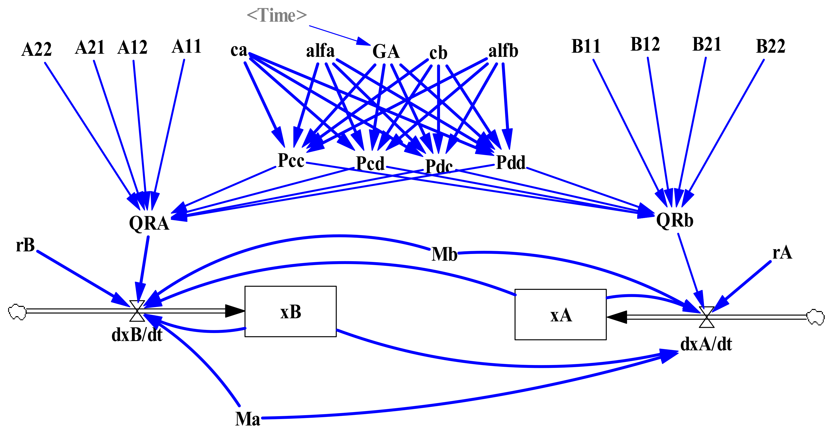
Figure 2 shows the framework of system dynamic simulations for different scenarios. This system includes two state variables $x_A$ and $x_B$, two flow rate variables $\raisebox{1ex}{$d{x}_A$}\!\left/ \!\raisebox{-1ex}{$dt$}\right.$ and $\raisebox{1ex}{$d{x}_B$}\!\left/ \!\raisebox{-1ex}{$dt$}\right.$, sixteen external variables, six intermediate variables, and one shadow variable (varying quantum entanglement parameter); start time INITIALTIME = 0, system simulation end time FINAL TIME = 60; simulation time step, TIME STEP = 1, and time unit generation. Here, all initial values meet the Stability conditions for competitive coexistence (

Table 7. Variables and initial values for the theoretical and simulation model.

Variable in Theoretical Model	Corresponding Variable in Simulation Model	Initial Value	Variable in Theoretical Model	Corresponding Variable in Simulation Model	Initial Value
${\mathit{A}}_{11}$	A11	1.5	${\mathit{M}}_{\mathit{A}}$	Ma	50
${\mathit{A}}_{12}$	A12	0.8	${\mathit{x}}_{\mathit{B}}$	xB	10
${\mathit{A}}_{21}$	A21	1.8	${\mathit{r}}_{\mathit{B}}$	rB	0.8
${\mathit{A}}_{22}$	A22	1.3	${\mathit{M}}_{\mathit{B}}$	Mb	50
${\mathit{B}}_{11}$	B11	1.4	${\mathit{\theta }}_{\mathit{A}}$	ca	180
${\mathit{B}}_{12}$	B12	1.7	${\mathit{\theta }}_{\mathit{B}}$	cb	0
${\mathit{B}}_{21}$	B21	0.7	${\mathit{\alpha }}_{\mathit{A}}$	alfa	0
${\mathit{B}}_{22}$	B22	1.2	${\mathit{\alpha }}_{\mathit{B}}$	alfb	90
${\mathit{x}}_{\mathit{A}}$	xA	10	$\mathit{\gamma }$	GA	40°
${\mathit{r}}_{\mathit{A}}$	rA	0.5

). In addition, to further investigate the impacts of higher payoffs (higher returns) on game outcomes, it is assumed that player A’s payoffs exceed player B’s payoffs. Entanglement parameter ($\gamma$), as a variable representing the entanglement intensity of interactive strategy, can be calculated as Equation (18), based on the aforementioned calculation steps and scenario setting and with its value meeting the game equilibrium and stable conditions for competition and cooperation coexistence. Thus, $\gamma =20°, 45° \mathrm{and} 70°$ are set in the simulations to disclose whether entanglement intensity affects the evolution trajectories of player population sizes and delineate the characteristics of those population size trajectories.

$$\left\{\begin{array}{l}Case 1: \gamma \in \left[0,\frac{\pi }{2}\right]\\ Case 2:\gamma \in \left[0,\frac{\pi }{2}\right]\\ \\ \left\{\begin{array}{l}Case 3: \gamma \in \left(33.21°,63.43°\right) \mathrm{in} \mathrm{competiton} coexistence\\ Case 3: \gamma \in \left[0,\frac{\pi }{2}\right] \mathrm{in} \mathrm{cooperation} coexistence \end{array}\right.\end{array}\right.$$

(18)

4.2. Scenario Simulation Results and Analysis

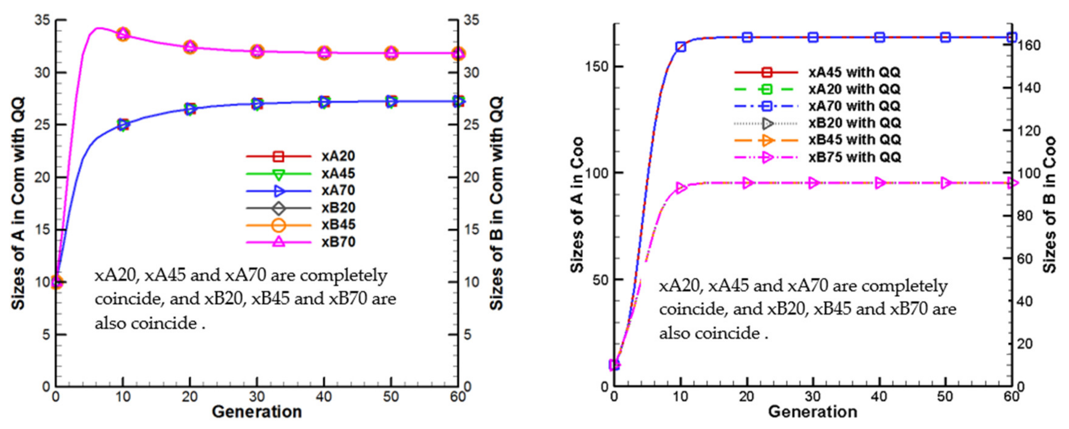
Figure 3 shows that, in case 1, player population sizes first rapidly increase and then evolve into a stable state whether the coexistence is competitive or cooperative in $\gamma {=20}^{°}, {45}^{°}{ \mathrm{and} 70}^{°}$. First, the population size evolution trajectories, whether for competitive or cooperative coexistence, are the same despite different $\gamma$ values. Second, in theory, player A with higher payoffs (higher returns) generally has more power than player B and thus the final and stable population size for player A is always larger than for player B whether the coexistence is cooperative or competitive. Meanwhile, the final population sizes for players in cooperative coexistence are larger than the initial environment capacity (M_a = 50, M_b = 50). However, population sizes for players in competitive coexistence are always smaller than the initial environment capacity (M_a = 50, M_b = 50).

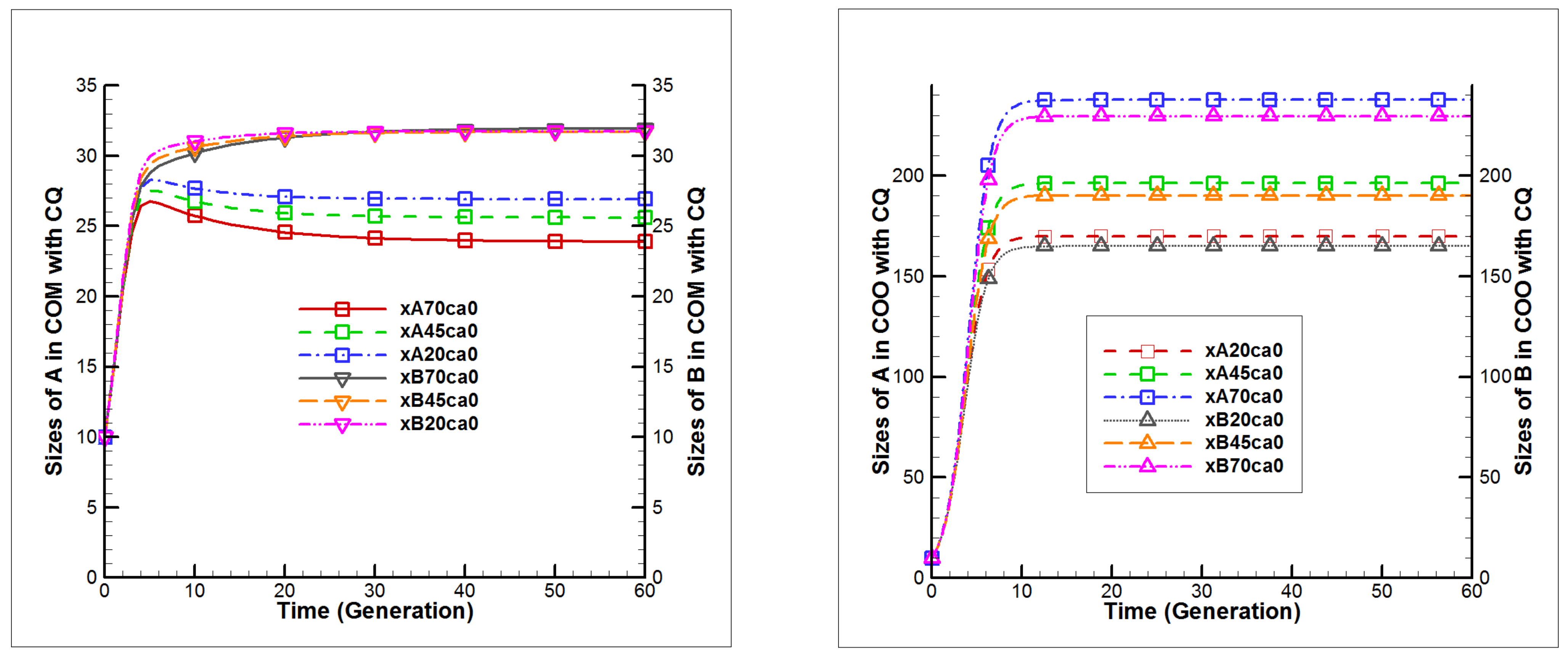
Figure 4 shows that, in case 2, the population sizes for each player first rapidly increase, and then evolve into a stable state whether the coexistence is competitive or cooperative. First, in competitive coexistence: the final and stable population sizes cannot break through the initial environment capacity (M_a = 50, M_b = 50); the entanglement intensity ($\gamma$) negatively affects the final population size for player A, but has no impact on the evolution of population size for player B; the final population size for player B is larger than for player A, even though the payoff for player A is higher than for player B, which reflects weaker players defeating stronger players in case 2. Second, in cooperative coexistence: the final population sizes for players surpasses the initial environment capacity; the entanglement intensity ($\gamma$) simultaneously and positively affects population sizes for the players; all final population sizes for player A are larger than for player B no matter the $\gamma$ value. Meanwhile, by contrast, final population sizes for players in cooperative coexistence are always larger than the initial environmental capacity, but always smaller than the initial environmental capacity in competitive coexistence. Furthermore, increasing entanglement intensity increases population sizes for players in cooperative coexistence, but constrains population sizes for players who initially take an independent strategy in competitive coexistence. In addition, in competitive coexistence, the final and stable population sizes for player B are larger than those for player A, even though player B has lower returns than player A, which reflects that, in some cases, weaker players can beat stronger players in competitive coexistence. However, in cooperative coexistence, the final population sizes for player A with higher payoffs are always larger than the final population sizes for player B, which illustrates that players with higher payoffs generally have more power in cooperative coexistence.

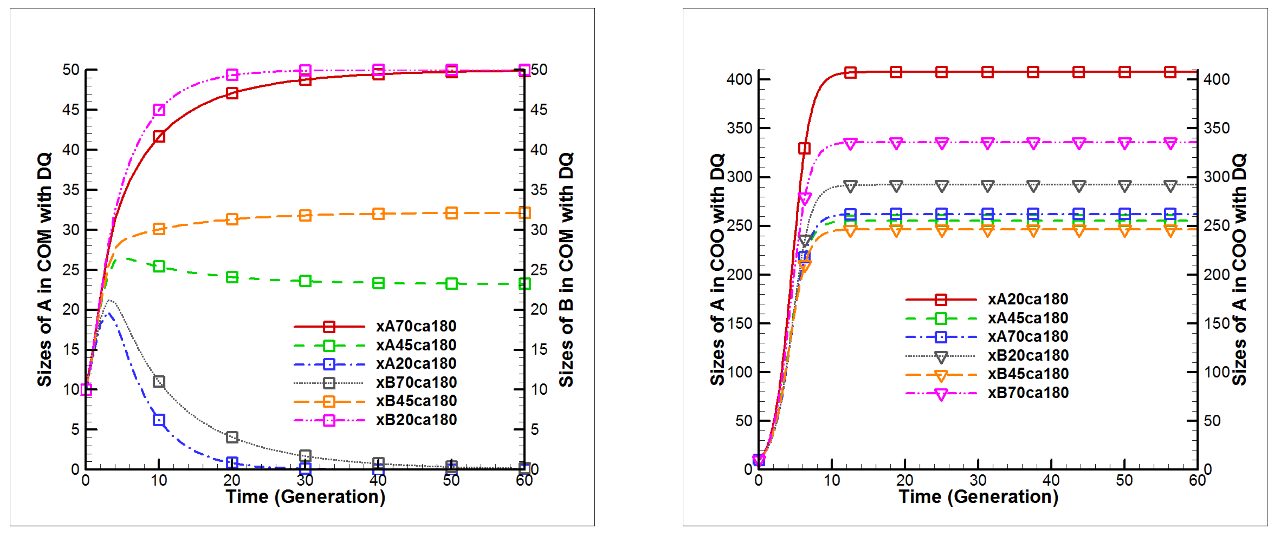
Figure 5 shows that, in case 3, the impacts of the entanglement intensity ($\gamma$) on the evolution trajectories and final population sizes for players vary with the entanglement intensity ($\gamma$). First, when $\gamma =20°$: in competitive coexistence, the population size for player A first rapidly increases and then rapidly decreases to nearly zero, but the population size for player B first rapidly increases and then slowly increases to about 50 (the initial environmental capacity); in cooperative coexistence, the population sizes for both players first rapidly increase and then slowly evolve into stable values, and both final and stable population sizes are larger than the initial environmental capacities. Second, when $\gamma =45°$: in competitive coexistence, the population sizes for both players first rapidly increase and then slowly decrease to stable values, less than the initial environmental capacity. Meanwhile, when $\gamma =70°$, in competitive coexistence, the population size for player A first rapidly increases and then slowly increases to a stable population size close to the initial environmental capacity, but the population size for player B first rapidly increases and then rapidly decreases to zero; in cooperative coexistence, the population sizes for both players first rapidly increase and then slowly stabilize, changing with entanglement intensity ($\gamma$), and all the final and stable population sizes for both players are larger than the initial maximum environmental capacity, but population size for player A is always larger than for player B.

In sum, the initial strategy state of players, payoffs and entanglement intensity obviously affect the evolution of population sizes for the players, with the obviously different characteristics between competitive and cooperative coexistence. First, the final and stable population sizes for players change with the initial strategy state, such as in cases 1 and 3, when $\gamma =20°$, in competitive coexistence, the final and stable population sizes for player A in case 1 is close to 27 and nearly zero in case 3, while the final and stable population sizes for player B in case 1 is close to 18 and close to 50 in case 3. Second, the entanglement intensity also plays a key role in the final and stable population sizes. For example, in case 3, when $\gamma =20°$, the final and stable population sizes for player A are close to zero, but the final and stable population sizes for player B almost reach the initial environmental capacity (50), even though the payoffs for player B are lower than for player A. Third, players with higher payoffs always have more strength in cooperative coexistence. Furthermore, all the final and stable population sizes for players in cooperative coexistence are larger than the initial environmental capacity. In contrast, all the final and stable population sizes for players in competitive coexistence are smaller than the initial environmental capacity. Finally, the results certify that players with higher payoffs in cooperative coexistence always are stronger in that coexistence, but not in competitive coexistence.

5. Discussion

The L–V model depicting population dynamics of ecological competitors has been continuously improved [14,15]. However, both the L–V model and the improved L–V models disregard the game initial strategy and strategy interactions. For example, in the improved model proposed by Novak et al. [14] or Huang et al. [15], the environment capacities are constant, strategies are independent, and the initial strategy is exogenous. In reality, human decisions follow quantum rules, are mutually dependent [27], and the entanglement intensity of strategy interactions and payoffs determine game equilibrium and stability [44]. Thus, our proposed model fills those knowledge gaps, not only by quantifying the entanglement intensity of strategy interactions, but also by taking the initial strategy and dynamic environment capacity into account. Most importantly, our scenario simulation results certify that the initial strategy, payoffs and entanglement intensity of strategy interactions codetermine the population dynamics for the players, game equilibrium and stability.

In particular, the impacts of the initial strategy, payoffs and entanglement intensity of strategy interactions on the final and stable population sizes differ between cooperative and competitive coexistence. First, in cooperative coexistence, all the population sizes finally evolve into a stable state and exceed the initial environment capacity in the three scenario simulations, but in competitive coexistence, all the population sizes are less than the initial environmental capacity. Furthermore, the disparities in the final and stable population sizes in the different scenarios within competitive or cooperative coexistence are decided by the initial strategy, payoffs and the entanglement intensity of strategy interactions. These findings prove that cooperative coexistence is beneficial to increasing population sizes for players and overcomes the constraints of the initial environmental capacity. As Nowak [45] determined, in cooperative coexistence all players are mutually beneficial. In addition, in an open and dynamic system, environmental capacity grows with social-economic development and technological progress. Thus, in cooperative coexistence, all the final and stable population sizes for players exceeded the initial environmental capacity due to the increased environmental capacity. However, in competitive coexistence, population sizes cannot break through their initial environmental capacity mainly because resource allocation is generally lower than in cooperative coexistence.

Furthermore, the scenario simulation results reveal that the entanglement parameter for the evolutionary trajectories of player population dynamics, determine the stability conditions for the coexistence equilibrium (Figure 4 and Figure 5). As Müller and Rau [46] affirmed, human decisions are interdependent mainly because human decisions are determined through different potential and non-potential conflicting motives and occur in an uncertain social environment. Importantly, our proposed model can be used to not only quantify the entanglement intensity but also delineate disparities in impacts of entanglement intensity on game outcomes in combination with different initial strategies. First, the scenario model results verify our hypothesis that the strategy evolution and game outcomes change since the initial strategy varies the entanglement intensity of strategy interactions as in case 2 (Figure 4) and case 3 (Figure 5). This finding agrees with the identification by Du et al. [45] that entanglement intensity dominates game outcomes, except in case 1 (Figure 3), when game outcomes were the same even with different entanglement intensities. However, these cases provide evidence to support the significance of the initial strategy on game outcomes.

Most studies asserted that players with higher payoffs are always stronger in the real world [14]. However, in reality, many large companies with higher payoffs have been beaten by smaller companies, and many weaker players overcome stronger players. Our findings provide evidence to better explain why weaker players can win. First, the results illustrate that players with higher payoffs may be beaten by their weaker competitors in competitive coexistence if players with higher payoffs initially disregard their weaker competitors and make their strategies independent from their competitors (Figure 5). The scenario simulation results indicate that the entanglement intensity $\gamma =20°$ ($\gamma =20°<33.31°$) leads stronger players to an extinct state in case 3 as the stronger players implement an initial independent strategy and continuously disregard their competitors in the game. Another interesting finding is that, in case 2 of competitive coexistence (Figure 4), the population sizes of players with higher payoffs are always larger than those of weaker players when $\gamma =70°$ ($\gamma =70°$ > $63.43°$). In other words, players with higher payoffs have stronger powers in coexistence once those higher payoff players decided to cooperate with their competitors when making their strategy. Walker and Hipel’s [47] findings support that players’ attitudes are a structure, which allows a decision analyst to consider the decision makers’ desires to hurt or help themselves or other decision makers, or to be neutral.

Most notably, compared to the improved L–V model, which uses evolutionary game theory, our model can simulate how players choose two pure strategies simultaneously, namely how players can choose strategy superposition by implementing cooperative and competitive strategies. That strategy state can be represented as state superposition by $\left|\psi \right.〉=\left(C_1\left|11\right.〉+C_2\left|01\right.〉+C_3\left|10\right.〉+C_4\left|00\right.〉\right)$ ($C_1,C_2,C_3,C_4$, is amplitude, ${\displaystyle \sum _{i=1}^4{C}_i^2}=1$). In reality, most players have implemented this type of strategy portfolio, which largely deviates from previous research based on classical and evolutionary game models because of the principle of set mutual exclusion in classical probability theory. One example of this tendency is the improved L-V model proposed by Huang [14], in which the single strategy selection only involves special cases and is inconsistent with actual situations.

6. Conclusions

In this study, based on the modified L–V model and quantum decision making theory, our proposed model incorporates the initial strategy state, payoffs and entanglement intensity of strategy interaction in an open social system, and can be used to investigate player population dynamics. Simulation results show that our proposed model can be used to interpret more realistic population dynamics in coexistence. One finding is that our proposed model is not constrained by the assumption of density-dependent mechanisms. Another finding is that our proposed model is not limited by the assumption of independent strategies. Our theoretical analyses show similar conclusions to those from a modified L–V model in that payoffs and entanglement intensity determine population dynamics, equilibrium and stability, and that player population sizes in cooperative coexistence would be larger than in competitive coexistence. Further, our results identify that the initial strategy, combined with the entanglement intensity of strategy interaction, play a vital role in game outcomes and game process, which greatly differs from the results from previous studies, which put aside the initial strategy state. Additionally, our results clearly reveal why stronger players may be defeated by the weaker competitors, at times, in the real world.

Understanding the influence of entanglement intensity on interactive strategy, initial strategy state, and payoffs on player population dynamics, equilibrium and stability should be regarded as an important step to elucidate player population dynamics in an open social system which more closely simulates reality. In this study, some limitations are worth noting. Although our model theoretically delineates the characteristics of population size evolution with strategy interaction, designing experimental methods to compute strategy interaction intensity is one of the key issues to be investigated in the future. Further study will empirically test our proposed model by designing experimental methods to estimate strategy interaction intensity.

References

1. Paul, S.; Mondal, S.P.; Bhattacharya, P. Numerical solution of Lotka Volterra prey predator model by using Runge–Kutta–Fehlberg method and Laplace Adomian decomposition method. Alex. Eng. J. 2016, 55, 613–617. [Google Scholar] [CrossRef] [Green Version]
2. Vadillo, F. Comparing stochastic Lotka–Volterra predator-prey models. Appl. Math. Comput. 2019, 360, 181–189. [Google Scholar] [CrossRef]
3. Zhang, G.; Allaire, D.; McAdams, D.A.; Shankar, V. System evolution prediction and manipulation using a Lotka-Volterra ecosystem model. Design. Stud. 2019, 60, 103–138. [Google Scholar] [CrossRef]
4. Bhargava, S.C. Generalized lotka-volterra equations and the mechanism of technological substitution. Technol. Forecast. Soc. 1989, 35, 319–326. [Google Scholar] [CrossRef]
5. Pretorius, L.; Pretorius, J.H.C.; Benade, S.J. A system dynamics approach to technology interaction: From asymptotic to cyclic behaviour. Technol. Forecast. Soc. 2015, 97, 223–240. [Google Scholar] [CrossRef]
6. Tsai, B. Predicting the competitive relationships of industrial production between Taiwan and China using Lotka-Volterra model. Appl. Econ. 2017, 49, 2428–2442. [Google Scholar] [CrossRef]
7. Zhang, W.; Lam, J.S.L. An empirical analysis of maritime cluster evolution from the port development perspective—Cases of London and Hong Kong. Transp. Res. A-Pol. 2017, 105, 219–232. [Google Scholar] [CrossRef]
8. Wang, H.; Wang, T. Application of the grey Lotka-Volterra model to forecast the diffusion and competition analysis of the TV and smartphone industries. Technol. Forecast. Soc. 2016, 106, 37–44. [Google Scholar] [CrossRef]
9. Hung, H.; Chiu, Y.; Huang, H.; Wu, M. An enhanced application of Lotka-Volterra model to forecast the sales of two competing retail formats. Comput. Ind. Eng. 2017, 109, 325–334. [Google Scholar] [CrossRef]
10. Tsai, B.; Chang, C.; Chang, C. Elucidating the consumption and CO2 emissions of fossil fuels and low-carbon energy in the United States using Lotka-Volterra models. Energy 2016, 100, 416–424. [Google Scholar] [CrossRef]
11. Hung, H.; Tsai, Y.; Wu, M. A modified Lotka-Volterra model for competition forecasting in Taiwan’s retail industry. Comput. Ind. Eng. 2014, 77, 70–79. [Google Scholar] [CrossRef]
12. Christodoulakis, N. Conflict dynamics and costs in the greek civil war 1946–1949. Defence Peace Econ. 2016, 27, 688–717. [Google Scholar] [CrossRef] [Green Version]
13. Cerqueti, R.; Tramontana, F.; Ventura, M. On the coexistence of innovators and imitators. Technol. Forecast. Soc. 2015, 90, 487–496. [Google Scholar] [CrossRef]
14. Huang, W.; Hauert, C.; Traulsen, A. Stochastic game dynamics under demographic fluctuations. Proc. Natl. Acad. Sci. USA 2015, 112, 9064. [Google Scholar] [CrossRef] [PubMed] [Green Version]
15. Novak, S.; Chatterjee, K.; Nowak, M.A. Density games. J. Theor. Biol. 2013, 334, 26–34. [Google Scholar] [CrossRef] [Green Version]
16. Manapat, M.L.; Nowak, M.A.; Rand, D.G. Information, irrationality, and the evolution of trust. J. Econ. Behav. Organ. 2013, 90, S57–S75. [Google Scholar] [CrossRef]
17. Nishimura, T.; Okada, A.; Shirata, Y. Evolution of fairness and coalition formation in three-person ultimatum games. J. Theor. Biol. 2017, 420, 53–67. [Google Scholar] [CrossRef]
18. Simon, H.A. A mechanism for social selection and successful altruism. Science 1990, 250, 1665–1668. [Google Scholar] [CrossRef] [Green Version]
19. Ye, W.; Fan, S. Evolutionary snowdrift game with rational selection based on radical evaluation. Appl. Math. Comput. 2017, 294, 310–317. [Google Scholar] [CrossRef]
20. Zhang, H. Errors can increase cooperation in finite populations. Game Econ. Behav. 2018, 107, 203–219. [Google Scholar] [CrossRef]
21. Friedman, D. On economic applications of evolutionary game theory. J. Evol. Econ. 1998, 8, 15–43. [Google Scholar] [CrossRef] [Green Version]
22. Smith, J.M.; Price, G.R. The logic of animal conflict. Nature 1973, 246, 15–18. [Google Scholar] [CrossRef]
23. Smith, J.M. Game theory and the evolution of behaviour. Proc. R. Soc. Lond. B Biol. Sci. 1979, 205, 475–488. [Google Scholar] [CrossRef] [PubMed]
24. Friedman, D. Evolutionary Games in Economics. Econometrica 1991, 3, 637–666. [Google Scholar] [CrossRef] [Green Version]
25. Wang, T.; Li, C.; Yuan, Y.; Liu, J.; Adeleke, I.B. An evolutionary game approach for manufacturing service allocation management in cloud manufacturing. Comput. Ind. Eng. 2019, 133, 231–240. [Google Scholar] [CrossRef]
26. Erol, M. Quantum Entanglement: Fundamentals and Relations with Consciousness/Mind. Neuroquantology 2010, 8, 390–402. [Google Scholar] [CrossRef]
27. Kazuo, K.; Keisuke, N. A Quantum Brain Model of Decision-Making Process Incorporated with Social Psychology. Neuroquantology 2019, 17, 72–76. [Google Scholar]
28. Chen, K.Y.; Hogg, T. How Well Do People Play a Quantum Prisoner’s Dilemma? Quantum. Inf. Process. 2006, 5, 43–67. [Google Scholar] [CrossRef]
29. Mihara, T. Information sharing using entangled states and its applications to quantum card tricks. Decis. Support Syst. 2011, 50, 522–528. [Google Scholar] [CrossRef]
30. Al-Nowaihi, A.; Dhami, S. The Ellsberg paradox: A challenge to quantum decision theory? J. Math. Psychol. 2017, 78, 40–50. [Google Scholar] [CrossRef] [Green Version]
31. Cheon, T.; Takahashi, T. Interference and inequality in quantum decision theory. Phys. Lett. A 2010, 375, 100–104. [Google Scholar] [CrossRef] [Green Version]
32. Eisert, J.; Wilkens, M.; Lewenstein, M. Quantum Games and Quantum Strategies. Phys. Rev. Lett. 1999, 83, 3077–3080. [Google Scholar] [CrossRef] [Green Version]
33. Yukalov, V.I.; Sornette, D. Quantitative Predictions in Quantum Decision Theory. IEEE Trans. Syst. Man Cybern. Syst. 2018, 48, 366–381. [Google Scholar] [CrossRef] [Green Version]
34. Kowalski, A.M. Betting on dynamics. Phys. A Stat. Mech. Appl. 2016, 458, 106–114. [Google Scholar] [CrossRef]
35. Pawela, L. Quantum games on evolving random networks. Phys. A 2016, 458, 179–188. [Google Scholar] [CrossRef] [Green Version]
36. Pawela, L.; Sladkowski, J. Cooperative quantum Parrondo’s games. Phys. D 2013, 256, 51–57. [Google Scholar] [CrossRef] [Green Version]
37. Horodecki, R.; Horodecki, P.; Horodecki, M.; Horodecki, K. Quantum entanglement. Rev. Mod. Phys. 2009, 81, 865–942. [Google Scholar] [CrossRef] [Green Version]
38. Busemeyer, J.R.; Wang, Z. What Is Quantum Cognition, and How Is It Applied to Psychology? Curr. Dir. Psychol. Sci. 2015, 24, 163–169. [Google Scholar] [CrossRef]
39. Bruza, P.; Kitto, K.; Nelson, D.; McEvoy, C. Is there something quantum-like about the human mental lexicon? J. Math. Psychol. 2009, 53, 362–377. [Google Scholar] [CrossRef] [PubMed] [Green Version]
40. Yukalov, V.I.; Sornette, D. Manipulating Decision Making of Typical Agents. IEEE Trans. Syst. Man Cybern. Syst. 2014, 44, 1155–1168. [Google Scholar] [CrossRef] [Green Version]
41. Guo, H.; Zhang, J.; Koehler, G.J. A survey of quantum games. Decis. Support Syst. 2008, 46, 318–332. [Google Scholar] [CrossRef]
42. Sun, Z.W. The Rule for Evolution of Cooperation in Quantum Games. Acta Phys. Pol. A 2009, 116, 135–140. [Google Scholar] [CrossRef]
43. Marinatto, L.; Weber, T. A quantum approach to static games of complete information. Phys. Lett. A 2000, 272, 291–303. [Google Scholar] [CrossRef] [Green Version]
44. Du, J.F.; Xu, X.D.; Li, H.; Zhou, X.Y.; Han, R.D. Entanglement playing a dominating role in quantum games. Phys. Lett. A 2001, 289, 9–15. [Google Scholar] [CrossRef]
45. Nowak, M.A. Five Rules for the Evolution of Cooperation. Science 2006, 314, 1560–1563. [Google Scholar] [CrossRef] [PubMed] [Green Version]
46. Müller, S.; Rau, H.A. Decisions under uncertainty in social contexts. Game Econ. Behav. 2019, 116, 73–95. [Google Scholar] [CrossRef] [Green Version]
47. Walker, S.B.; Hipel, K.W. Strategy, Complexity and Cooperation: The Sino-American Climate Regime. Group Decis. Negot. 2017, 26, 997–1027. [Google Scholar] [CrossRef]
Figure 1. Schematic diagram of the quantum game calculation. (Note: this schematic diagram is mainly referred to Eisert et al. 1999).
Mathematics 09 02217 g001
Figure 2. Schematic diagram of system dynamics simulation of the improved L–V model.
Mathematics 09 02217 g002
Figure 3. Evolution trajectories for player population sizes in case 1. (Note: QQ is for case 1; 20, 45, and 70 are the different entanglement intensities; Coo and Com are the cooperation and competition coexistence, respectively; xA20 and xB20, xA45 and xB45, and xA70 and xB70 are the evolution trajectories of player A and B population sizes with entanglement intensity 20°, 45° and 70°, respectively).
Mathematics 09 02217 g003
Figure 4. Evolution trajectories for player population sizes in case 2. (Note: ca0 is case 2; 20, 45, and 70 equal different entanglement intensities; Coo and Com are cooperation and competition coexistence, respectively; xA20 and xB20, xA45 and xB45, and xA70 and xB70 are the evolution trajectories of player A and B population sizes with entanglement intensity 20°, 45° and 70°, respectively).
Mathematics 09 02217 g004
Figure 5. Evolution trajectories for player population sizes in case 3. (Note: ca180 is case 3; 20, 45, and 70 equal different entanglement intensities; Coo and Com are cooperation and competition coexistence, respectively; xA20 and xB20, xA45 and xB45, and xA70 and xB70 are the evolution trajectories of player A and B population sizes with entanglement intensity 20°, 45° and 70°, respectively).
Mathematics 09 02217 g005